Generalizing trigonometric functions from different

Generalizing trigonometric functions from different points of view David Edmunds, Jan Lang March 2009 In this survey we shall explore (one definition of) generalized trigonometric functions from different standpoints and illustrate the roles they play in various branches of mathematics. We start from the analytic point of view and for each p ∈ (1, ∞) introduce a function sin−1 p by an integral formula, which is just an extension of the well known integral representation of arcsin, and then use it to define generalized sine, cosine and tangent functions (labelled sinp , cosp and tanp respectively). Numerous properties of these functions, such as an identity of Pythagorean type, are exhibited. Then we consider the unit circle in R2 with the lp norm and define generalized trigonometric functions as is done in the standard case when the l2 norm is used. We show that these functions coincide with those introduced earlier. In the third section R x we consider the integral operator T : Lp (I) → Lp (I) given by T f (x) = 0 f (t)dt, where I = (0, 1), and look at the problem of finding an extremal function (an element of the unit sphere of Lp (I) at which the norm of T is attained). It turns out that the extremal functions are given by cosp . The following section deals with the Dirichlet eigenvalue problem for the p−Laplacian on a bounded interval: all eigenfunctions are expressible by means of sinp functions, which corresponds exactly to the classical situation when p = 2. After establishing a connection with approximation theory, we conclude with a review of other ways in which the classical trigonometric functions have been generalized. In the literature a variety of different definitions of generalized trigonometric functions can be found (see [7], [8]): all extend the classical functions and preserve some of their properties. It becomes clear that no single definition preserves all the classical properties and that which definition is adopted depends on the applications envisaged. Our focus on a particular choice reflects our research interests.

1

Analytic point of view

It is well known from basic calculus that Z 1 1 √ dt = π/2 1 − t2 0 1

(1)

and

Z 0

x

√

1 dt, 1 − t2

0≤x≤1

(2)

1 define a (differentiable) function on [0, 1]. Since √1−t is positive on (0, 1), the 2 function is increasing and one-to-one from [0, 1] to [0, π/2]. This function is arcsin(x) and can be used to define the function sin on [0, π/2]. By standard extension procedures we can define the sin function on (−∞, ∞). Obviously this can be extended. Let 1 < p < ∞ and define a (differentiable) function Fp : [0, 1] → R by Z x 1 √ dt, 0 ≤ x ≤ 1. (3) Fp (x) = p 1 − tp 0

Since Fp is strictly increasing it is a one-to-one function on [0, 1] with range [0, πp /2], where Z 1 1 √ πp = 2 dt, 0 ≤ x ≤ 1. (4) p 1 − tp 0 The inverse of Fp on [0, πp /2] we denote by sinp and extend as in the case of sin (p=2) to [0, πp ] by defining sinp (x) = sinp (πp − x)

for x ∈ [πp /2, πp ];

further extension is achieved by oddness and 2πp -periodicity on the whole of R. By this means we obtain a differentiable function on R which coincides with sin when p = 2. Corresponding to this we define a function cosp by the prescription cosp (x) =

d sinp (x), x ∈ R. dx

(5)

Clearly cosp is even, 2πp -periodic and odd about πp ; and cos2 = cos. If x ∈ [0, πp /2], then from the definition it follows that cosp (x) = (1 − (sinp (x))p )1/p .

(6)

Moreover, the asymmetry and periodicity show that | sinp (x)|p + | cosp (x)|p = 1,

x ∈ R.

(7)

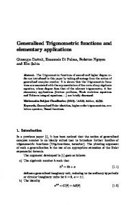
Fig.1 below gives the graphs of sinp and cosp for p = 1.2 and 6. From (4) it follows that Z 1 πp = p−1 (1−sp )−1/ps1/p−1 ds = p−1 B(1−1/p, 1/p) = p−1 Γ(1−1/p)Γ(1/p), 2 0 where B is the Beta function, Γ is the Gamma function and πp =

2π . p sin(π/p) 2

(8)

Figure 1: sin6 , cos6

and

sin1.2 , cos1.2

Clearly π2 = π and, with p0 = p/(p − 1), pπp = 2Γ(1/p0 )Γ(1/p) = p0 πp0 .

(9)

Using (8) and (9) we see that πp decreases as p increases, with lim πp = ∞,

p→1

lim (p − 1)πp = lim πp0 = 2.

lim πp = 2,

p→∞

p→1

p→1

(10)

The dependence of πp on p is illustrated in Fig. 2.

Figure 2: y = πp The generalized tangent function is defined as in the classical case: tanp x =

3

sinp x . cosp x

(11)

Figure 3: y = tan6 (x),

[0, π6 /2)

y = tan1.2 (x),

[0, π1.2 /2)

Fig.3 indicates the behaviour of tanp when p = 1.2 and 6. Obviously tanp x is defined for all x ∈ R except for the points (k + 1/2)πp (k ∈ Z); it is odd, πp -periodic and tanp 0 = 0. Use of (7) shows that on (−πp /2, πp /2), tanp has derivative 1 + | tanp x|p . It follows that 1 d (tan−1 p x) = dx 1 + |x|p and on (−πp /2, πp /2), Z x 1 dt tan−1 (x) = p p 0 1 + |t| Evidently tan−1 2 x = arctan x.

2

Geometric point of view

Here we start by recalling the definition of the sin and cos functions via the unit circle in the plane R2 with the l2 metric, and then generalize this for R2 with the lp metric. Given r > 0, then Sr = {(x, y) ∈ R2 ; x2 + y 2 = r2 } is a circle in the plane 2 R with the l2 metric. Each point in R2 can be described by rectangular coordinates (x, y) or polar coordinates (r, φ). The relation between these different coordinates is described by the functions sin, cos and tan. The connection between polar and rectangular coordinates is given by: x =

r cos(φ)

(12)

y

r sin(φ).

(13)

=

Due to the l2 metric we have r 2 = x2 + y 2 ; 4

and φ is related to x and y by means of the tan function: φ = tan−1 (y/x), when x, y > 0. Let us consider the case p 6= 2.

Figure 4: The first quadrant of S1 for p = 2, 6, 1.2 Then the analogue of the circle is the p−circle Sr = {(x, y) ∈ R2 ; |x|p +|y|p = r } and we expect the following identities: p

x

= r cosp (φ)

(14)

y

= r sinp (φ).

(15)

From this follows | sinp (φ)|p +| cosp (φ)|p = 1, so that cosp (φ) = (1−(sinp (φ))p )1/p when x, y > 0. Fig. 4 above shows how the shape of S1 changes with p. When p 6= 2, the p−circle Sr is not symmetric with respect to rotation and then the obvious one-to-one relation between the length of a curve segment on Sr and its angle, as we have in the l2 metric, does not exist. Instead of this we will consider the quite natural condition d sinp (φ) = cosp (φ), dφ setting φ = 0 when (x, y) = (1, 0), and suppose that φ increases when (x, y) moves on Sr in the anticlockwise direction. Then 1 1 d sin−1 = when 0 ≤ t < 1, p (t) = −1 dt 1 − tp cosp (sinp (t)) from which it follows that the sinp and cosp functions defined in this section are the same as those defined in Section 1.

5

We define the tanp function as in Section 1: tanp (φ) :=

sinp (φ) cosp (φ)

and we have, as in the l2 case, φ = tan−1 p (y/x), when x, y > 0.

3

An integral operator and generalized trigonometric functions

In this section we concentrate on the most simple integral operator. On the interval I = [0, 1] let Z x T f (x) := f (t)dt. (16) 0

At first we consider T as a map from L2 (0, 1) into L2 (0, 1). It is obvious that T is compact and that there exists a function in L2 (0, 1) at which the norm of T is attained. In this case it is quite simple to show that kT |L2 (0, 1) → L2 (0, 1)k = 2/π and that the norm is attained when:  πx  π f (t) = cos 2 2 so that T f (t) = sin

 πx 

. 2 When p 6= 2 then again T is a compact map from Lp (0, 1) into Lp (0, 1) and there exists a function at which the norm is attained. In [6] it was proved that 1 1− p10 + p

kT |Lp (0, 1) → Lp (0, 1)k =

(p0 + p)

and that the norm is attained when: π x π p p f (t) = cosp and 2 2

0

(p0 )1/p p1/p 1 1 B( p0 , p )

T f (t) = sinp

π x p . 2

This leads us, again, to the generalized trigonometric functions.

4

Eigenfunctions for the p-Laplacian

Consider the following classical Dirichlet problem on (0, 1) :  ∆u + λu = 0 on (0, 1), u(0) = 0, u(1) = 0.

6

(17)

It is well known that all eigenvalues are of the form: λn = (nπ)2 ,

n∈N

with corresponding eigenfunctions un (t) = sin (nπt) ,

n ∈ N.

We recall the definition of the p-Laplacian which is a natural extension of the Laplacian: ∆p u = (|u0 |p−2 u0 )0 . Evidently ∆2 u = ∆u. Then the analogue of (17) is the eigenvalue problem  ∆p u + λ|u|p−2 u = 0 on (0, 1), (18) u(0) = 0, u(1) = 0. In [4] it is shown that all eigenvalues of this problem are of the form λn = (nπp )p

p p0

with corresponding eigenfunctions un (t) = sinp (nπp t). Once more we see the appearance of our generalized trigonometric functions. Let us note that the literature on the p-Laplacian and operators that resemble it in some sense is enormous. Here we mention only a few works, beyond those already cited, that seem of particular relevance to our approach. Of particular interest is the excellent survey paper by Lindqvist [11]; see also the book [5]. In [1] a Sturm-Liouville theory is developed for the one-dimensional p-Laplacian, following on from the work of [3]; see also [12].

5

The approximation theory point of view and the generalization of trigonometric functions

Let 1 < p < ∞ and −∞ < a < b < ∞. Consider the Sobolev embedding on I = [a, b], (19) E : W01,p (I) → Lp (I), where W01,p (I) is the Sobolev space of functions on the interval I with zero trace equipped with the following norm: ku|W01,p (I)k :=

Z

1

1/p |u0 (t)|p dt .

0

The Sobolev embedding is one of the most useful maps in Analysis. It is well known that (19) is a compact map and that more detailed information about its 7

compactness plays an important role in different branches of mathematics. The properties of compact maps can be well described by using the Kolmogorov, Bernstein and Gel’fand n-widths together with the approximation numbers. We recall the definitions of these quantities: Definition 5.1 Let T : X → Y be a bounded operator, where X and Y are Banach spaces, and let n ∈ N. (i) The Kolmogorov n-width dn (T ) of T is inf kT x − ykY

dn (T ) = dn (T (X), Y ) = inf sup

Xn kxkX ≤1 y∈Xn

where the infimum is taken over all n-dimensional subspaces Xn of X. (ii) The Gel’fand n-width dn (T ) of T is dn (T ) = dn (T (X), Y ) = inf n L

kT xkY

sup kxkX ≤1,x∈Ln

where the infimum is taken over all subspaces Ln of codimension n of X. (iii) The Bernstein n-width bn (T ) of T is bn (T ) = bN (T (X), Y ) = sup

inf

Xn+1 T x∈Xn+1 ,T x6=0

kT xkY /kxkX

where Xn+1 is any subspace of span{T x : x ∈ X} of dimension ≥ n + 1. (iv) The approximation number an (T ) of T is an (T ) = inf kT − F |X → Y k, where the infimum is taken over all bounded linear maps F : X → Y with rank less than n. In our case we have X = W01,p (I) and Y = Lp (I). Then since Lp (I) has the approximation property for 1 ≤ p ≤ ∞, E is compact if and only if am (E) → 0 as m → ∞. h i h i h i |I| 1 |I| 1 |I| , In = b − 21 |I| , b and I = a + (i − ) , a + (i + ) Define I0 = a, a + 2n i n 2 n 2 n for 1 < i < n. Then {Ii }ni=0 is a covering of I and we use it to define the following map: n−1 X Rn f = Pi f i=1

where Pi f (x) = χIi (x)f

  |I| a+i . n

It is obvious that Rn is a map from W01,p (I) into Lp (I) with rank = n − 1. The following theorem was proved in [2]. 8

Theorem 5.2 Let 1 < p < ∞. Then |I| sn (E) = · nπp



p0 p

1/p

and sn (E) = k(E − Rn )g|Lp (I)k, where g(x) = sinp



x − a |I| πp n



and sn (E) stands for any of the following: an (E), dn (E), dn (E) or bn (E). This theorem provides us with information about the image of the unit ball of W01,p (I) in the space Lp (I). We can see from this theorem that the largest element in BW01,p (I) := {f ; kf |W01,p k ≤ 1} in the Lp (I) norm is   sinp x−a |I| πp   f1 (x) := . x−a k sinp πp |I| |W01,p (I)k Let us approximate BW01,p (I) by a one-dimensional subspace in Lp (I). The most distant element from the optimal one-dimensional approximation is   |I| · sinp x−a πp 2   . f2 (x) := x−a |I| k sinp πp 2 |W01,p (I)k More generally, if we approximate BW01,p (I) by an n-dimensional subspace in Lp (I), then the most distant element from the optimal n-dimensional approximation is   |I| sinp x−a πp · n   . fn (x) := |I| 1,p k sinp x−a |W (I)k 0 πp n Also from the previous theorem we have that kfi kLp (I) = sn (E) We can see that the functions fi are playing, in some sense, roles similar to those of the semi-axes of an ellipsoid. We present below figures which show an image of BW01,p (I) restricted to a linear subspace span{f1 , f2 , f3 } in Lp (I). In the case p = 2 we obtain an ellipsoid (here the x, y, z axes correspond to f1 , f2 , f3 ).

9

Figure 5: p = 2 When p = 10 and p = 1.1 we have the images below:

Figure 6: p = 10

p = 1.1

We can see that the main difference between Fig. 5 and Fig 6 is that the pictures in Fig. 6 are not convex. This suggests that possibly the functions f1 , f2 , f3 are not orthogonal in the James sense. We recall the definition of this orthogonality. Let a, b be elements of a Banach space X. We say that a is orthogonal to b in the James sense, written a ⊥j b, if kakX ≤ ka + λbkX for every λ ∈ R. In some literature this orthogonality is called Birkhoff orthogonality. Fig. 7 indicates that for p = 6 (similar graphs can be obtained for other p 6= 2) the function f1 is not orthogonal to f3 and also f3 is not orthogonal to f1 .

10

Figure 7: f (t) = kf1 + tf3 kp

6

f (t) = kf3 + tf1 kp

Some other definitions of generalized trigonometric functions

The definition of the generalised trigonometric functions that we have chosen is only one of several that can be found in the literature, which is now quite extensive and goes back at least as far as the 1879 work of Lundberg (see [10]): details of the various approaches can be found in the papers of Lindqvist [9] and of Lindqvist and Peetre [7] ; see also [8]. In [10] a beautiful account is given of the history of such work, with especial reference to that of Lundberg. To illustrate these alternative methods we consider first the approach taken in [7], [8]. Let p∈ (1, ∞) and set 1

Z π fp = p

0

dt . (1 − tp )(p−1)/p

On (0, π fp /p) define functions Sp , Cp , and Tp by: Z x= 0

Sp (x)

dt , p (1 − t )(p−1)/p

Z

1

x= Cp (x)

dt , p (1 − t )(p−1)/p

Z x= 0

Tp (x)

dt (1 + tp )2/p

and extend them to R as was done in Section 1. Note that π fp = pSp−1 (1) = pCp−1 (0). Then we have, on (0, π fp /p), Sp (x)p + Cp (x)p = 1,

Tp (x) =

Sp (x) Cp (x)

Sp0 (x) = C(x)p−1 , Cp0 (x) = −S(x)p−1   π fp Sp − x = Cp (x), p

11

(20)

 Sp

π fp 2p



1 = √ = Cp p 2



π fp 2p

 .

(21)

When p = 2, we see that S2 (x) = sin(x), C2 (x) = cos(x), T2 (x) = tan(x). Another way of proceeding is given in [9] (see also the earlier paper [13]). In this we set √ 2pp−1 π. π ˆp = p sin πp On (0, π ˆp /2) we define functions Sˆp (x), Cˆp (x), and Tˆp (x) by: ˆp (x) S

Z x= 0

Z

dt (1 −

tp

p−1 )

, 1/p

Z

√ p

p−1

x= ˆp (x) C

Tˆp (x)

x= 0

dt

(1 −

tp 1/p , p−1 )

dt tp 1 + p−1

and extend them to R as in Section 1. Note that p p

π ˆp p − 1 = Sˆp ( ) = Cˆp (0). 2

When p = 2 clearly Sˆ2 (x) = sin(x), Cˆ2 (x) = cos(x), Tˆ2 (x) = tan(x). We have on (0, π ˆp /2): 0 (Cˆp0 (x))p (Sˆp (x))p + =1 p0 − 1 p−1

and

0 dSˆp (x) = (p − 1)1/p (Cˆp0 (x))p −1 dx ˆ 0 dCp (x) = −(p − 1)1/p (Sˆp0 (x))p −1 dx     π ˆ π ˆ Sˆp (x) = Cˆp − x , Cˆp (x) = Sˆp −x , 2 2

while for Tˆp we have Tˆp (x) = and also

ˆ

Sp (x) d ˆ dx (Sp (x))

=

Sˆp (x) , (p − 1)1/p (Cˆp0 )p0 −1

 (Tˆp (x))p d ˆ Tp (x) = 1 + . dx p−1

However, it is important to recognise that whatever definition is adopted, good features will be accompanied by less pleasant ones. For example, the 12

definition used in the earlier sections leads to the fine Pythagorean identity (7) and has a close connection with the Dirichlet problem for the p−Laplacian, but the derivative of cosp is given by a somewhat complicated formula and πp → ∞ as p → 1. The definition given first in the present section leads to the Pythagorean relation and to the property (20), but the derivative of Sp involves a power of Cp . As for the last definition, while π bp remains bounded as p varies, to set against that is the fact that the Pythagorean relation is not bp are given by expressions aesthetically pleasing and the derivatives of Sbp and C without much appeal. The choice of definition to be made depends on how best the features of the corresponding generalised function fit in with the particular application envisaged.

References [1] Binding, P. and Dr´ abek, P., Sturm-Liouville theory for the p-Laplacian, Studia Sci. Math. Hungar. 40 (2003), 375-396. [2] Edmunds, D. E.; Lang, J., Behaviour of the approximation numbers of a Sobolev embedding in the one-dimensional case. J. Funct. Anal. 206 (2004), no. 1, 149–166. ´ A half-linear second order differential equation, in Qualitative [3] Elbert, A., theory of differential equations, Vol. I,II (Szeged, 1979), pp. 153-180, Colloq. Math. Soc. J´ anos Bolyai, 30, North-Holland, Amsterdam-New York, 1981. [4] Dr´ abek, P.; Man´ asevich, R. On the closed solution to some nonhomogeneous eigenvalue problems with p-Laplacian. Differential Integral Equations 12 (1999), no. 6, 773–788. [5] Dr´ abek, P., Kufner, A. and Nicolesi, F., Nonlinear elliptic equations, Univ. West Bohemia, Pilsen, 1996. [6] Levin, V.I., On a class of integral inequalities, Recueil Math´ematiques 4 (46) (1938), 309–331. [7] Lindqvist, Peter; Peetre, Jaak,; p-Arclength of the q-Circle, Preprints in Mathematical Csiences 2000:21, Lund University. [8] Lindqvist, Peter; Peetre, Jaak; Borwein, Jonathan M.; Problems and Solutions: Solutions: Generalized Trigonometric Functions: 10744 Amer. Math. Monthly 108 (2001), no. 5, 473–474. [9] Lindqvist, Peter, Some remarkable sine and cosine functions Ricerche Mat. 44 (1995), no. 2, 269–290 (1996). [10] Lindqvist, P. and Peetre, J., Comments on Erik Lundberg’s 1879 thesis, especially on the work of G¨oran Dillner and his influence on Lundberg,

13

Mem. dell’Istituto Lombardo, Accad. Sci. e Lett., Classe Sci. Mat. Nat. XXXI, Fasc. 1, Milano 2004. [11] Lindqvist, P., Notes on the p-Laplace equation, Report, Univ. of Jyv¨askyl¨a, Dept. Math. and Statistics, 102, Jyv¨askyl¨a 2006, pp. ii+80. ˆ [12] Otani, M., A remark on certain nonlinear elliptic equations, Proc. Fac. Sci. Tokai Univ. 19 (1984), 23-28. [13] Peetre, Jaak; The differential equation y 0p − y p = ±1 (p > 0), University of Stockholm, Department of Mathematics, Report No 12, 1992 ¨ [14] Schmidt, E., Uber die Ungleichung, welche die Integrale u ¨ber eine Potentz einer Funktion und u ¨ber eine andere Potenz ihrer Ableitung verbindet, Math. Ann. 117 (1940), 301-326.

14