Abstract. Computerized adaptive testing (CAT) is a powerful technique to help improve mea- surement precision and reduce the total number of items required in ...
JSS
Journal of Statistical Software July 2016, Volume 71, Issue 5.
doi: 10.18637/jss.v071.i05
Generating Adaptive and Non-Adaptive Test Interfaces for Multidimensional Item Response Theory Applications R. Philip Chalmers York University
Abstract Computerized adaptive testing (CAT) is a powerful technique to help improve measurement precision and reduce the total number of items required in educational, psychological, and medical tests. In CATs, tailored test forms are progressively constructed by capitalizing on information available from responses to previous items. CAT applications primarily have relied on unidimensional item response theory (IRT) to help select which items should be administered during the session. However, multidimensional CATs may be constructed to improve measurement precision and further reduce the number of items required to measure multiple traits simultaneously. A small selection of CAT simulation packages exist for the R environment; namely, catR (Magis and Raîche 2012), catIrt (Nydick 2014), and MAT (Choi and King 2014). However, the ability to generate graphical user interfaces for administering CATs in realtime has not been implemented in R to date, support for multidimensional CATs have been limited to the multidimensional three-parameter logistic model, and CAT designs were required to contain IRT models from the same modeling family. This article describes a new R package for implementing unidimensional and multidimensional CATs using a wide variety of IRT models, which can be unique for each respective test item, and demonstrates how graphical user interfaces and Monte Carlo simulation designs can be constructed with the mirtCAT package.
Keywords: MIRT, CAT, multidimensional CAT, R, GUI.
1. Introduction Computerized adaptive testing (CAT) is a methodology designed to reduce the length of educational, psychological, and medical tests. In contrast to fixed linear tests (e.g., paperand-pencil forms, or digital surveys where questions are administered in sequence), CATs
2
Generating CAT Interfaces for MIRT Applications
attempt to select optimal items based on selection rules that capitalize on pre-calibrated item information and the participants’ provisional trait estimates (Weiss 1982). Throughout a CAT session, the trait estimates are updated as the responses to items are collected. The trait estimates serve as a basis in determining which items should be administered next, and the associated standard errors for the estimates help inform whether the CAT session should be terminated early. In common CAT designs, items are administered when they are believed to effectively reduce the expected standard error of measurement of the latent trait values. Administering items which optimally reduce the standard error of measurement helps to create efficient test forms that improve the measurement reliability for a given participant by using a smaller subset of test items (Wainer and Dorans 2000). In order to implement CATs effectively, various item-level characteristics must be known a priori. Specifically, the parameters required to operationalize the item selection process, as well as to compute provisional latent trait estimates, are generally adopted from the item response theory paradigm (IRT; Lord 1980). IRT parameters can be estimated for tests containing unidimensional or multidimensional latent trait structures, and offer a parametric mechanism to model the interaction between participants and item characteristics (Reckase 2009). CATs based on a unidimensional latent trait assumption have been extensively studied in methodological literature; however, with the advent of modern computing power, multidimensional CATs are becoming more popular (Reckase 2009). Multidimensional CATs (MCATs) are a useful alternative to administering multiple unidimensional CATs in situations where the traits are correlated (Segall 1996) or when items simultaneously capture variation in multiple traits (i.e., have “cross-loadings” in the vernacular of linear factor analysis; Mulaik 2010). Correlations between latent traits provide additional information about the locations of auxiliary traits, and in turn help to improve the overall measurement precision between the trait estimates. Due to the increase in statistical information, MCATs will often require fewer items than independently administered unidimensional CATs to reach the same measurement precision (Mulder and Linden 2009). Several important prerequisites are required before building interfaces to be used for MCATs. A cursory overview of these prerequisites include: • Obtaining a suitable item pool. The item pool (or bank) is a relatively large set of items that can be selected from during an MCAT application. The associated item parameters must have been calibrated for the population of interest beforehand using multidimensional IRT software (e.g., the mirt package in R Chalmers 2012, or an equivalent). In situations where more than one population will be administered items from the pool, all items should contain limited to no differential functioning to ensure that the selection of items is unbiased (Chalmers, Counsell, and Flora 2016; Wainer and Dorans 2000). • Initializing the MCAT session. Before an MCAT session can begin, initial latent trait estimates and hyper-parameter distribution definitions are generally required. The initial trait estimates often serve as the basis for selecting the initial item (if the initial item was not explicitly declared), while the hyper-parameter distributions are included as an added information component in the item selection process. The hyper-parameters are also included to add prior distributional information when updating the ability estimates throughout the MCAT session. When there is little to no prior information about the ability estimates, the starting values are generally selected to equal the mean of the latent trait distribution (often this is simply a vector of zeros).
Journal of Statistical Software
3
• Selecting the next item to administer. Several criteria have been proposed for unidimensional CATs to select optimal items for ability and classification designs, many of which have been implemented in unidimensional CAT software in R (e.g., see Magis and Raîche 2012). Fewer MCAT criteria have been proposed in the literature, though a small number of criteria are available. MCAT selection methods include the determinantrule (D-rule), trace of the information or asymptotic covariance matrix (T-rule and A-rule, respectively), weighted composite rule (W-rule), eigenvalue-rule (E-rule), and the Kullback-Leibler divergence criteria (Kullback and Leibler 1951). Due to their importance in MCAT applications, these criteria are explained in more detail below. • (Optional) – Selecting a pre-CAT design. Because MCAT estimation methods are based on responses to previous items, it can be desirable to run a “pre-CAT” stage before beginning the actual MCAT. In the pre-CAT stage, a small selection of items are administered under more controlled settings to ensure that, during the MCAT stage, the methods have enough information to be properly executed. • Selecting the IRT scoring method. Multiple criteria have been defined for obtaining provisional trait estimates. These criteria include: maximum-likelihood (ML) estimation, evaluating the expected or maximum values of the a posteriori distribution, weighted likelihood estimation, and several others (Bock and Aitkin 1981; Warm 1989). However, ML estimation requires special care because it cannot be used if responses are at the extreme ends of the categories (i.e., all-correct, all-incorrect). One possible solution to this issue is to use Bayesian methods (such as maximum a posteriori estimation) until a sufficient amount of variability in the responses are available for proper ML estimation. Another potential solution when selecting the ML algorithm is to include a pre-MCAT stage to collect responses until suitable ML estimates can be obtained. • Terminating the application. Deciding how to terminate an MCAT session is important for many practical reasons. MCATs may be terminated according to multiple criteria in a single session. For example, terminating a test based on the standard error of measurement is desirable if inferences about the precision of each latent trait estimate is required, though for multidimensional models the choice of whether this criteria should be applied globally or specifically for each latent trait must be specified. Tests may also be terminated after a specific number of items have been administered, the time allotted for answering the test has expired, the latent traits can be classified as above or below a set of predetermined latent cutoff values (Eggen 1999), and so on. Much of the superficial information listed above is also important for unidimensional CAT applications. Conversely, literature relevant to unidimensional CATs will largely be relevant for MCATs because they share the same underlying methodology. Therefore, additional information regarding MCAT methodology can largely be obtained from previous CAT publications, such as Magis and Raîche (2012) and the references therein. A small number of R packages exist for studying CAT designs through Monte Carlo simulations, including catR (Magis and Raîche 2012) and catIrt (Nydick 2014), which exclusively focus on unidimensional IRT models, and MAT (Choi and King 2014), which exclusively investigates the properties of the multidimensional three-parameter logistic model (M3PL). Hitherto, these packages have provided useful simulation tools for Monte Carlo research of
4
Generating CAT Interfaces for MIRT Applications
CAT design combinations with homogeneous IRT models; however, they have not been organized for real-time implementation of CATs, do not provide resources to build graphical user interfaces (GUIs), exclusively support either unidimensional or multidimensional CATs, and do not support mixing different classes of IRT models into CAT designs. As more R packages are developed for studying unidimensional and multidimensional CATs, a number of pertinent features remain missing. The mirtCAT package described in this article has been designed to address many of these missing features in the R environment. Specifically, mirtCAT provides front-end users with functions for generating CAT GUIs to be used in their research applications, and includes several tools for investigating the statistical properties of heterogeneous CAT designs by way of Monte Carlo simulations. The remainder of this article describes the theory behind applying MCATs, provides examples of how Monte Carlo simulation studies can be organized with the code from the package, and demonstrates how real-time unidimensional and multidimensional CATs – as well as standard questionnaire designs – can be generated to collect item response data.
2. Multidimensional computerized adaptive testing A number of multidimensional IRT models have been proposed for dichotomous and polytomous response data. For ease of presentation, we will only focus on the multidimensional four-parameter logistic model (M4PL) for dichotomous responses (coded as 0 and 1 for incorrect and correct answers, respectively), which is an extension of the multidimensional three-parameter logistic model (Reckase 2009), and the multidimensional nominal response model for polytomous items (Thissen, Cai, and Bock 2010). Multidimensional IRT models often contain a unidimensional counterpart as a special case when only one latent trait is modeled; therefore, the following theory relates to unidimensional IRT models as well.1 The probability that a participant positively endorses the j-th dichotomous item with an M4PL structure is Pj (y = 1|θ) = Pj (y = 1|θ, aj , dj , gj , uj ) = gj +
uj − gj , 1 + exp(−(aj> θ + dj ))
(1)
where the complementary probability for answering the item incorrectly is Pj (y = 0|θ) = 1 − Pj (y = 1|θ). The gj and uj parameters are restricted to be between 0 and 1 (where gj < uj ), and serve to bound the probability space within gj ≤ Pj (y = 1|θ) ≤ uj . The g parameter is useful when there is a non-zero probability for participants to randomly guess an item correctly. The uj parameter, on the other hand, controls the probability that participants will carelessly answer an item incorrectly. The multidimensional two-parameter logistic model (M2PL) can be recovered from Equation 1 when the gj and uj are fixed to 0 and 1, respectively, and the multidimensional three-parameter model (M3PL) is realized when fixing only uj to 1. Finally, θ is taken to be a D-dimensional vector of random ability or latent trait values, dj is the item intercept parameter representing the relative item “easiness”, and aj is a vector of slope parameters that modulate how θ influences the probability function. The multidimensional nominal response model (MRNM) can be used to model K-unordered 1 Although only two IRT models are presented below, in principle many other IRT models may be substituted in empirical applications.
Journal of Statistical Software
5
polytomous response categories that are coded k = 0, 1, . . . , K − 1. This model has the form �
exp αjk aj> θ + djk
Pj (y = k|θ) = Pj (y = k|θ, aj , αj , dj ) = P K−1 k=0
�
�
exp αjk aj> θ + djk
�,
(2)
where the aj and θ terms have the same interpretation as in Equation 1. Equation 2 contains unique intercept values (djk ) and so-called “scoring” parameters (αjk ) for each respective category. For identification purposes, the first element of djk and αjk are often constrained to be equal to 0, while the last element of αjk is constrained to be K − 1. The αjk values represent the relative ordering of the categories; larger αjk values indicate that the category has a stronger relationship with higher levels of θ. When specific constraints are applied to Equation 2, various specialized IRT models can be recovered. For instance, when the scoring parameters are constrained to have equal interval spacing (αj = 0, 1, 2, . . . , K − 1) the multidimensional generalized partial credit model (MGPCM) is realized, and when K = 2 the MRNM will become equivalent to the M2PL model.
2.1. Predicting latent trait scores After item responses have been collected, various estimates for θ can be computed. The θˆ estimates are obtained using the observed item responses, the item trace-line functions given their respective item parameters (ψj ), and (potentially) prior distributional information about θ. Multiple methods exist for obtaining θˆ values, such as weighted and unweighted maximum-likelihood estimation (WLE and ML, respectively; Bock and Aitkin 1981; Warm 1989), Bayesian methods such as the expectation or maximum of the posterior distribution (EAP and MAP, respectively; Bock and Aitkin 1981), and several others which have seen less use in applied settings (e.g., EAP for sum scores; Thissen, Pommerich, Billeaud, and Williams 1995). ML estimation of θ for a given response pattern requires optimizing the likelihood function l(y|θ, ψ) =
j −1 J KY Y
Pj (y = k|θ, ψj )χjk ,
(3)
j=1 k=0
where χjk is a dichotomous indicator variable (coded as 0 or 1) used to select the probability terms corresponding to the endorsed categories. In practice, however, it is generally more effective to use the log of Equation 3,
LL(y|θ, ψ) =
j −1 J KX X
χjk · log [Pj (y = k|θ, ψj )] .
(4)
j=1 k=0
Optimizing the log-likelihood directly results in ML estimates; however, obtaining a possible maximum requires that y contain a mix of 0 to Kj − 1 responses across the J items. If there is no variability in the response vector, such that SD(y) = 0, then θˆ will tend to −∞ or ∞ during optimization. Bayesian methods generally do not from suffer this particular limitation because they include additional information about the distribution of θ through a prior density function, φ(·), with hyper-parameters, η. The posterior function utilized in Bayesian prediction methods is l(y|θ, ψ)φ(θ|η) π(θ|y, ψ, η) = R , l(y|θ, ψ)φ(θ|η)
(5)
6
Generating CAT Interfaces for MIRT Applications
where Equation 5 is either integrated across to find the EAP estimates or maximized to find the MAP estimates. In multidimensional IRT applications, the prior density function is typically assumed to be from the multivariate Gaussian family with mean vector µθ and covariance matrix Σθ ; however, other multivariate density functions are possible. ˆ a measure of precision is required to make inferences about Following the computation of θ, the statistical precision of the estimates. As is the case with standard ML estimation theory, computing a quadratic approximation of the curvature in Equation 4 provides a suitable ˆ is determined measure of the parameter variability (Fisher 1925). The computation of VAR(θ) by inverting the D × D matrix of second derivatives with respect to θ (also known as the Hessian or negative of the observed information matrix), 2 ˆ ˆ = Σ(θ|y, ˆ ψ) = − ∂ LL(y|θ, ψ) VAR(θ) ∂θ∂θ >
!−1
.
(6)
Standard error estimates for each element in θˆ are then obtained by taking the square-root of ˆ ψ). If the log of Equation 5 each diagonal element in the asymptotic covariance matrix, Σ(θ|y, is used instead of Equation 4 then prior information about θ will also be included in the computation of the Hessian. Due to the added statistical information in Bayesian methods, ˆ ψ, η) will generally provide slightly smaller standard errors when an informative prior Σ(θ|y, distribution is included in the computations.2
2.2. Item selection for MIRT models Selecting optimal items in MCATs is generally more complicated than unidimensional CATs because items should only be selected if they effectively improve the precision of multiple traits. In this section, we focus on item selection methods that are tailored towards obtaining ˆ for all individuals sampled. An interesting area that is not investigated the lowest SE(θ) in this section is when items are selected so to optimally classify individuals above or below predefined cutoff values. Although various methods exist for unidimensional models, classification-based applications for MCATs have rarely been investigated in the literature and continue be an important area for future research (Reckase 2009). Selecting items according to the maximum information principle (Lord 1980) requires evaluating the Fisher-information matrix for each remaining item in the pool. The Fisher information is defined as ! ∂ 2 LL(y|θ, ψ) F(θ) = −E (7) ∂θ∂θ > where the inverse of Equation 7 serves as another suitable measure to approximate sampling variability of θ. For notational clarity, the vector of parameters ψ is omitted from the following presentation because the item parameters are assumed to be constant. F(θ) is useful in MCAT applications because it contains no reference to the observed response patterns, and therefore can be used to predict the amount of expected information contributed by items that have not been administered. However, in MCAT applications θ is not known beforehand; therefore, ˆ are used instead as plausible stand-ins for θ. The θˆ values are provisional estimates (θ) continually updated throughout the MCAT session to provide better approximates to the 2 ˆ is the actually posterior standard deviation of the trait estimates, PSD(θ). ˆ The Bayesian analogue of SE(θ) For simplicity, however, in the remainder of the text the two terms are used interchangeably.
Journal of Statistical Software
7
unobserved θ values. Because the precision about θ improves as more items are administered, the Fisher information criteria will in turn progressively select more suitable items for the unobserved latent trait values. As outlined in work by Segall (1996), selecting the most informative item requires evaluating ˆ for each of the M remaining items in the item pool. Due to the local independence F(θ) assumption in IRT (Lord 1980), the information contributed by the addition of the m-th item is additive, such that ˆ = FJ (θ) ˆ + Fm (θ), ˆ FJ+m (θ) (8) ˆ is the sum of the information matricies for the previously answered items. The where FJ (θ) matrix in Equation 8 is evaluated for the m = 1, 2, . . . , M remaining items in the pool. The M information matrices are then compared by reducing the multidimensional information to suitable scalar values according to how the joint variability should be quantified. If prior distribution information is included in the selection process then the following formula can be used to compute a Bayesian variant of the expected information (Segall 1996) ˆ = FJ (θ) ˆ + Fm (θ) ˆ − (∂ 2 log(φ(θ|η)))−1 . FJ+m (θ)
(9)
In the situation where a multivariate normal prior distribution is included, Equation 9 can be expressed as ˆ = FJ (θ) ˆ + Fm (θ) ˆ + Σ−1 . FJ+m (θ) (10) θ ˆ One potentially optimal approach to quantify the amount of joint item information in FJ+m (θ) is to select the item which provides the largest matrix determinant. The item with the maxiˆ mum determinant indicates which item provides the largest increase in the volume of FJ (θ); ˆ consequently, this selection property will maximally decrease the overall volume in ΣJ (θ) as ˆ = F −1 (θ) ˆ (Segall 1996). This criterion is called the “D-rule”, and is more well, where ΣJ (θ) J
formally expressed as �
�
ˆ |FJ+2 (θ)|, ˆ . . . , |FJ+M (θ)| ˆ . D-rule = max |FJ+1 (θ)|,
(11)
ˆ Another potentially useful criterion for selecting items is the maximum trace of FJ+m (θ), �
�
ˆ Tr(FJ+2 (θ)), ˆ . . . , Tr(FJ+M (θ)) ˆ . T-rule = max Tr(FJ+1 (θ)),
(12)
ˆ it does select While the T-rule does not guarantee the largest reduction in volume for ΣJ (θ), items which increase the average unweighted information about the latent traits, and also allows for unequal domain score weights to be applied if certain latent traits are deemed to be more important a priori. Applying weights to the T-rule helps to measure important traits more accurately because items will be selected with greater frequency if they measure the traits of interest. A closely related selection criterion to the T-rule is the asymptotic covariance rule, or A-rule (Mulder and Linden 2009), which selects items based on the minimum ˆ (potentially weighted) trace of ΣJ+m (θ), �
�
ˆ Tr(ΣJ+2 (θ)), ˆ . . . , Tr(ΣJ+M (θ)) ˆ . A-rule = min Tr(ΣJ+1 (θ)),
(13)
Much like the T-rule, the A-rule does not guarantee the maximum increase in the volume of the information matrix. Instead, the A-rule attempts to reduced the marginal expected standard
8
Generating CAT Interfaces for MIRT Applications
error for each θˆ by ignoring the covariation between traits. Next, the eigenvalue rule (Erule) has been proposed to select the item which minimizes the general variance of the ability ˆ estimates by selecting the smallest possible value from the set of eigenvalues in each ΣJ+m (θ). However, the E-rule may not optimally select items in a way that maximally reduces the standard error of measurement for all latent traits, and in general is not recommended for routine use (Mulder and Linden 2009). Finally, the W-rule can be used to select the maximum ˆ of the weighted information criteria, W = w> FJ+m (θ)w, where w is a weight vector subject > to the constraint 1 w ≡ 1 (Linden 1999). As with the optional weights for the T-rule and A-rule, the W-rule is an effective selection mechanism when specific latent traits should have lower measurement error than other traits. An alternative approach to selecting items using the Fisher information given provisional θˆ values is the Kullback-Leibler information (Chang and Ying 1996). This approach has the potential benefit over traditional information-based methods in that it can account for uncertainty of the θˆ values when only a small number of items have been administered (Chang and Ying 1996). The Kullback-Leibler information is KL(θ||θ0 ) = Eθ0 (LL(y|θ0 ) − LL(y|θ)) ,
(14)
where θ0 is the vector of true ability parameters, and the double bars in KL(θ||θ0 ) signify that θ and θ0 should be treated distinctly. Chang and Ying (1996) suggested that Equation 14 √ should be evaluated over the range θ ± ∆n , where ∆n may decrease by a factor of n as the number of items administered increases. A numerical integration approach is also possible for the Kullback-Leibler information, though for multidimensional IRT models this may be less useful because of the (often cumbersome) numerical evaluation of the integration grid across all latent trait dimensions (see Reckase 2009, p. 335, for a similar observation about evaluating the KL information in MCATs).
2.3. Exposure control and content balancing An unfortunate consequence when maintaining item pools is that informative items are often selected with greater frequency than less informative items. Exposing a smaller selection of items too often may lead to item security issues, loss of investments for items that are rarely selected, or in some cases may cause a decrease in content validity coverage due to reduced item sampling variability. Selection methods can be adjusted by including “exposure control” methods to help avoid overusing highly informative items (Linden and Glas 2010). Several methods of exposure control exist, though perhaps the most intuitive approach is the method proposed by McBride and Martin (1983). In their method, McBride and Martin suggest sampling from the n most optimal items (given the selection criteria) rather than simply selecting the most optimal item, and further recommend gradually reducing n as the examinee progresses through the test (the so-called 5-4-3-2-1 approach). This helps generate item variability in earlier stages of the test where item overexposure is more likely to occur. Simulation-based item exposure methods, such as the Sympson-Hetter (SH) approach (e.g., Veldkamp and Linden 2008), provide a different approach to controlling item overexposure. The SH method requires items to be pre-assigned a fixed value ranging from 0 to 1, and during the CAT session a simulation experiment is performed to determine whether or not a selected item is to be administered. For instance, after an optimal item is determined from the item pool, a random uniform value (r) is then drawn and compared to the item’s assigned
Journal of Statistical Software
9
SH value. If r is less than the assigned SH value then the item is administered, otherwise it is discarded from the item pool and the next most optimal item undergoes the same simulation experiment; this process continues until an item is selected and administered. Unfortunately, it is not clear whether more advanced exposure control methods outperform simple heuristic methods in empirical settings (e.g., see, Revuelta 1998). An undesirable side-effect when implementing exposure control methods is that there is loss of item selection efficiency, and in most applications this loss of efficiency will require more items to be administered before termination criteria based on the standard error of measurement can be obtained. Using exposure control early in the MCAT session, where it often is most important, also generates uncertainty about selection methods that theoretically should perform well earlier in the CAT session (such as the Kullback-Leibler criteria). Another area of interest when administering test items is the use of “content balancing” to ensure that specific types of item content appear during the CAT session. Content balancing generally involves the classification of items to predetermined groups, and these groups are assigned a proportion or percentage value relating to how often the content groups should appear in the CAT session. A simple yet effective method for content balancing, proposed by Kingsbury and Zara (1991), involves comparing the empirically obtained content proportions to the desired content proportions. After computing the selection criteria for each remaining item in the item pool, the proportion of items in the content domains for all the items previously administered are subtracted from the desired content domain percentages for the respective domains. The content domain that has the largest difference between the desired proportion is then selected, and the item with the most optimal selection criteria within the selected domain is then administered. This approach ensures that content balancing is efficiently achieved throughout the session while quasi-maintaining the optimal item selection criteria. Content balancing methods mainly have been studied in unidimensional CAT applications, however they can be applied equally well to MCATs. Fortunately, MCAT designs can implicitly offer a suitable approach to balancing content domains. As Segall (1996) explained, an MCAT session primarily intended to measure one trait could be organized to form a bifactor structure (e.g., Gibbons and Hedeker 1992; Gibbons et al. 2007) to achieve a content balancing effect. Within the bi-factor model, each content grouping can be organized as a specific latent trait, where item slopes only relate to the respective subsets of homogeneous content groupings. Given the bi-factor structure, items could then be selected using criteria that weight the selection process in favor of selecting items which measure the general trait, while also including information about the specific traits; this would result in a probabilistic selection mechanism for sampling the content domains indirectly with the item selection criteria. Of course, practitioners may still wish to include more traditional content balancing methods if other properties of the test should be selected. In this case, multiple content balancing methods could be combined to form a balanced sampling design. For instance, in addition to selecting specific contents with the bi-factor design, a CAT session may also be organized to contain 80% multiple-choice questions, 10% reading comprehension questions, and 10% fill-in-the-blank questions, and these proportions can be controlled using Kingsbury and Zara’s (1991) method.
10
Generating CAT Interfaces for MIRT Applications
2.4. Termination criteria In the interest of time, item bank security, and avoiding fatigue effects, one or more stopping criteria should be included in MCATs. One reasonable approach to terminating the MCAT application is to require all SE(θˆk ) ≤ δ, where δ is a maximally tolerable standard error of measurement for all the latent traits. However, if some elements in θˆ should be measured with more precision then unique δk values for each θˆk value should be defined. For example, if the MCAT is organized to contain a bi-factor structure then the test developer may wish to terminate the session when only the primary trait reaches a predefined δk value. Unequal δk values should be used in conjunction with the W-rule, weighted T-rule, or weighted A-rule, so that items which accurately measure the traits of interest are selected with greater frequency. Classification-based criteria also exist for terminating MCATs when cutoff values are supplied for each trait. In classification-based MCATs, the session may be terminated when the confidence intervals (given 1 − α) for each θˆ do not contain the pre-specified cutoff values. When ˆ do not contain the cutoff values then the individuals may be classified as above or the CI (θ)s below the cutoff values for the respective traits, otherwise the MCAT results will suggest that not enough information exists to reject the plausibility of the cutoffs. More specific methods for terminating CATs are also possible (e.g., use of loss functions or risk analyses), however these are not explored in this article. Finally, termination criteria can be based on other practical considerations as well, such as setting the maximum number of items that can be administered in a given session, stopping the CAT after a specific amount of time has elapsed, the θˆ values are changing very little as new items are added, and so on.
3. The mirtCAT package The mirtCAT package (available from the Comprehensive R Archive Network at https: //CRAN.R-project.org/package=mirtCAT) provides tools for test developers to generate GUIs for CATs as well as functions for Monte Carlo simulation studies involving CAT designs. mirtCAT uses the HTML generating tools available in the shiny package (RStudio Inc. 2014) to generate real-time CATs for interactive sessions within standard web-browsing software. The mirtCAT package builds and extends upon the estimation tools available in the mirt package (Chalmers 2012), and provides a wide range of support for any mixture of unidimensional and multidimensional IRT models to be used for CATs. Currently supported models in mirtCAT include unidimensional and multidimensional versions of the 4PL model (Lord 1980), the graded response model and its rating scale counterpart (Muraki 1992; Muraki and Carlson 1995; Samejima 1969), the generalized partial credit and nominal model (Thissen et al. 2010), the partially compensatory model (Chalmers and Flora 2014; Sympson 1977), the nested-logit model (Suh and Bolt 2010), the idealpoint model (Maydeu-Olivares, Hernández, and McDonald 2006), and polynomial or product constructed latent trait combinations (Bock and Aitkin 1981). Additionally, the mirt package supports the use of prior parameter distributions, linear and non-linear parameter constraints (e.g., see, Chalmers 2015), and specification of fixed parameter values; hence, nested versions of the previously mentioned models can be estimated from empirical data. For instance, the 1PL model (Thissen 1982) can be formed in mirt because it is a highly nested version of the M4PL model with equality constraints for the slope parameters.
Journal of Statistical Software
11
3.1. A simple non-adaptive GUI example The mirtCAT package generates interactive GUIs to run CATs by providing inputs to the mirtCAT() function. When generating a GUI, the mirtCAT() function requires a data.frame object containing questions, response options, and output types. When only a data.frame is supplied, a non-adaptive test (i.e., a survey) will be initialized because no IRT parameters were defined for selecting the items adaptively. Currently, the required inputs names in the data.frame object are: • Question – A character vector containing all the question stems. • Option.# – Possible response options for each item, where # corresponds to the specific category. For instance, a test with 4 unique response options for each item would contain the columns “Option.1”, “Option.2”, “Option.3”, and “Option.4”. If some items have fewer categories than others then NA placeholders must be used to omit the unused options. • Type – Indicates the type of response input to use from the shiny package. The supported types are: "radio" for radio buttons, "select" for a pull-down box for selecting inputs, "text" for requiring typed user input, "checkbox" for collecting multiple checkboxes of responses for each item, "slider" for slider-style inputs, and "none" when only an item stem should be presented. • Answer or Answer.# – (Optional) A character vector (or multiple character vectors) indicating the scoring key for items that have correct answers. If there is no correct answer for a question then NA values must be specified as placeholders. When a checkbox type is used with this input then responses are scored according to how many matches were selected. • Stem – (Optional) A character vector of absolute or relative paths pointing to external markdown (.md) or HTML (.html) files, which can be used as item stems. NAs are used if the item has no corresponding file. • ... – Additional optional argument inputs that are passed to the associated shiny construction functions. For the "slider" input, however, a column for the "min", "max", and "step" arguments must be defined. When generating surveys with mirtCAT, only the Type, Question, and Option inputs are typically required. If questions are to be scored in real time (as they generally are in ability measuring CATs) then a suitable Answer vector must be supplied. Finally, if specific graphical stimuli should be included then the paths pointing to the item-stem files must be included in the Stem input. Before generating a real-time CAT GUI, it is informative to first generate a simple survey to highlight the fundamental mirtCAT() inputs. For example, say that a researcher wishes to build a small survey with only three rating scale items, where each item contains five ratingscale options ranging from “Strongly Disagree” to “Strongly Agree”. Initializing the HTML interface to collect responses can be accomplished with the following code: R> library("mirtCAT") R> options questions df results R> R> R> R> R> + R>
a responses fscores(mirt_object, response.pattern = responses, method = "ML") Item.1 Item.2 Item.3 Item.4 Item.5 Item.6 Item.7 Item.8 Item.9 0 1 1 1 0 1 1 1 1 Item.10 F1 SE_F1 [1,] 0 0.4609681 0.8596507 [1,]
Because all items were administered, the unsorted response pattern is identical to the pattern generated from generate_pattern(). If items were not responded to due to early termination of the CAT then NA values would be present in the items containing no observations.
4. Single case MCAT example In this section, an MCAT design and graphical user interface are constructed using the code located in Appendix A. The questions and item parameters were arranged to emulate how a multidimensional mathematical achievement test with cross-factor loadings and correlated latent traits could be managed. The item bank consisted of 120 items in total, and a data.frame object with the questions and answers was included. The first 30 items were constructed to measure only a hypothetical “Addition” trait, while the last 30 items measured only on a “Multiplication” trait. The middle 60 items were evenly split to contain a mix of the Addition and Multiplication slopes. However, the first half of these items were designed to relate more to the Addition trait (contained larger slopes), while the last 30 items were designed to
Journal of Statistical Software
Test Information
21
Test Standard Errors 45 0.45
40 0.40 40 35
0.40
0.35
0.35
30
30
I(θ)
SE(θ) 0.30 20
25
0.30
0.25
0.20
10
20 0.25 3
3 15
2
1
1 0
θ2
2
2
3
0
1
−1
0
10
−1
−2 −3
−2 −3
θ2
2
0.20
0 −1
−2 −3
θ1
3
1
−1 −2 −3
θ1
5
0.15
Figure 3: Plots of test implied response functions from models estimated in the mirt package. relate more to the Multiplication trait. The expected information and standard error plots below indicate that respondents with abilities closer to the center of the distributions will be measured with the most accuracy, while those in the more extreme ends of the ability range will be measured with much less precision. R> plot(mod, type = "info", theta_lim = c(-3, 3)) R> plot(mod, type = "SE", theta_lim = c(-3, 3)) The resulting plots are shown in Figure 3. Given the objects defined in Appendix A, we first generate a plausible observed response pattern for a participant with abilities θ = [−0.5, 0.5]. R> set.seed(1) R> pat head(pat) [1] "145" "195" "200" "232" "207" "175" The character responses indicates that, among the options in df[1, ], the category pertaining to the option "145" was selected as the correct answer, "195" was selected for the second item among the possible options in df[2, ], and so on for the remaining 118 items. To determine how the MCAT session would behave if each item were administered in sequence, the min_items argument could be increased to ensure that all items are selected; alternatively, the min_SEM input could be decreased to a much smaller value to accomplish the same goal. R> result print(result)
22
Generating CAT Interfaces for MIRT Applications CAT Standard Errors
Theta_1
Theta_2
1.0
●
0.5
●
●
●
● ●● ● ●
● ●
0.0
● ●
● ●
● ●
θ
● ●
●
● ● ●
−0.5
●
●
●
● ● ● ●●● ● ● ● ● ● ● ● ●● ●● ● ● ● ●● ●
● ●
●● ●
●
●●● ● ● ● ● ● ● ●
● ● ●●
●
●● ●● ●● ● ● ● ●● ●●● ● ● ● ● ● ● ● ● ●●● ● ●● ●
● ●
●● ● ●●● ● ● ● ● ●●● ● ● ● ● ●● ● ● ●● ●● ● ● ● ● ● ● ● ● ●● ● ● ● ● ● ● ● ● ●● ● ●● ● ● ●●● ●● ●● ● ● ●●
● ● ● ● ●● ● ●● ● ●● ● ● ● ●●●●●●●●●●●●●●●●●●●●●●●●●●●●●●● ● ●●●● ●●●●●● ●● ●●●●●●●●●●●●●●●●●●
●
●
●
−1.0
Item
Figure 4: Estimated θ values and standard errors in dependence of items administered. n.items.answered Theta_1 Theta_2 SE.Theta_1 SE.Theta_2 120 -0.3700409 0.3307961 0.2382641 0.1991176 R> plot(result, scales = list(x = list(at = NULL)) The plot is shown in Figure 4. Some initial observations can be made from inspecting the graphical output generated by plot(result). By design, the test parameters were simulated to almost exclusively measure the Addition trait for the first 60 items, and the consequences of this are clearly seen in the ability estimates and their respective standard errors. The standard errors for Theta_1 rapidly decreased in the first half of the test, while the standard errors for Theta_2 stayed roughly the same until the second half of the test began3 . As well, the point estimates for Theta_1 were able to move closer towards the population value of −0.5 in the first half, but only after the second half of the test began does Theta_2 begin to move towards the population value of 0.5. Although not shown above, the results from summary(results) revealed that both traits were measured with a standard error less than 0.4 after the 73rd item was administered. Administering all items in an item pool is generally not desirable in real testing situations when the item parameters are available. Therefore, we will instead implement a multidimensional adaptive test design to select items that are more suitable for the observed response pattern. First, we choose an MCAT item selection criteria to help maximally increase the information in both traits simultaneously. Because the latent traits are deemed to be of equal importance 3
Had the latent traits been orthogonal the second trait estimates and standard errors would have remained completely stationary. However, because the traits are slightly correlated, information about the first trait will provide indirect information about the second trait.
Journal of Statistical Software
23
in this example, the use of the D-rule for selecting items is a reasonable choice. Next, we set the stopping criteria for the standard error of measurement to 0.4 for all traits. The response pattern previously simulated is then reanalyzed in mirtCAT() with R> set.seed(1234) R> MCATresult print(MCATresult) n.items.answered Theta_1 Theta_2 SE.Theta_1 SE.Theta_2 18 -0.5315822 0.7334699 0.3922312 0.3525484 R> summary(MCATresult) $final_estimates Theta_1 Theta_2 Estimates -0.5315822 0.7334699 SEs 0.3922312 0.3525484 $raw_responses [1] "3" "2" "1" "3" "3" "5" "5" "3" "1" "3" "3" "1" "1" "3" "4" "1" "5" "4" $scored_responses [1] 1 0 0 1 0 1 1 0 1 1 1 1 1 1 0 1 1 0 $items_answered [1] 40 118 59 $thetas_history Theta_1 [1,] 0.0000000 [2,] 0.3300104 [3,] 0.1417429 [4,] -0.3095254 [5,] -0.2671319 [6,] -0.6102685 [7,] -0.3903506 [8,] -0.3774346 [9,] -0.5382688 [10,] -0.5065322 [11,] -0.4950992 [12,] -0.4864141 [13,] -0.3538263 [14,] -0.3480257 [15,] -0.3465018 [16,] -0.4941311
65
41
3
93
Theta_2 0.000000000 0.279113425 -0.280431989 -0.381602240 -0.118300123 -0.162056553 -0.144267168 0.003104662 -0.006176610 0.176070232 0.384451064 0.521754123 0.527263358 0.626719891 0.697100900 0.690762595
31
87
63 107
24
96
82
5
15 110
21
24 [17,] -0.4398394 [18,] -0.4374101 [19,] -0.5315822
Generating CAT Interfaces for MIRT Applications 0.693084295 0.737414618 0.733469944
$thetas_SE_history Theta_1 Theta_2 [1,] 1.0000000 1.0000000 [2,] 0.8676229 0.9072747 [3,] 0.8150130 0.5880719 [4,] 0.6409551 0.6047584 [5,] 0.6340877 0.4731553 [6,] 0.5635720 0.4760173 [7,] 0.4990944 0.4734596 [8,] 0.4982264 0.4252720 [9,] 0.4648866 0.4251890 [10,] 0.4618842 0.3967178 [11,] 0.4609951 0.3806421 [12,] 0.4605138 0.3706390 [13,] 0.4363271 0.3715648 [14,] 0.4364367 0.3653976 [15,] 0.4365725 0.3593208 [16,] 0.4196257 0.3580614 [17,] 0.4045024 0.3584700 [18,] 0.4045165 0.3533521 [19,] 0.3922312 0.3525484 For this particular response pattern, the MCAT session was terminated after only 18 items were administered. As can be seen from the summary results above, and the generated plot below, the items were effectively selected so to reduce the standard error estimates more rapidly. Improving the standard errors consequently improves the rate at which the point estimates converge to their population values. When compared to administering items in an ordered sequence, the MCAT with the D-rule criteria was able to obtain the same degree of measurement precision with 55 fewer items. Clearly, even for a small test bank such as the one simulated here, the payoff to implementing MCATs can be quite meaningful compared to more traditional item selection methods (see Figure 5). R> plot(MCATresult)
4.1. Customizing GUI elements To demonstrate how the previous MCAT example can be transformed into a useful GUI, we will now focus on the related graphical inputs required for the mirtCAT() function. The code in Appendix A generated character vectors for the questions, options, and answers for 120 items, and placed these values in an objected called df. The df object can be passed to the mirtCAT(df = ...) input, which will generate simple text-based question stems using suitable HTML code. However, in the code below we will include two additional items to demonstrate how more stimulating item stems can be presented. When defining items, test
Journal of Statistical Software
25
CAT Standard Errors 0
40
118
59
65
41
3
93
31
Theta_1
87
63
107
24
96
82
5
15
●
●
●
110
21
●
●
Theta_2
1.0
● ●
0.5
●
● ● ● ●
θ
●
0.0
●
●
● ● ● ●
●
●
●
● ●
●
●
●
●
● ●
−0.5
●
●
●
87
63
●
●
● ●
●
−1.0
0
40
118
59
65
41
3
93
31
107
24
96
82
5
15
110
21
Item
Figure 5: Estimated θ values and standard errors in dependence of items administered. designers will often wish to present stimuli other than the default text output, and instead include materials in the form of images, tables, maps, and so on. In such cases, the df input may include a Stem character vector to point to previously defined markdown or HTML files. The following code adds two items to the existing df object which point to external HTML files. The rbind.fill() function from the plyr package (Wickham 2011) is used below to quickly fill in missing values with NAs, which can be useful when combining two data.frame objects. Screen captures of the graphical item stems can be seen in Figure 6. R> R> R> + R> R> R> + + R> R> R> R>
type