Hindawi Publishing Corporation Journal of Applied Mathematics Volume 2013, Article ID 302680, 7 pages http://dx.doi.org/10.1155/2013/302680
Research Article Generating Irregular Models for 3D Spherical-Particle-Based Numerical Methods Gang-Hai Huang,1 Yu-Yong Jiao,1 Xiu-Li Zhang,1 Amoussou-Coffi Adoko,1 and Shu-Cai Li2 1
State Key Laboratory of Geomechanics and Geotechnical Engineering, Institute of Rock and Soil Mechanics, Chinese Academy of Sciences, Wuhan 430071, China 2 Geotechnical & Structural Engineering Research Centre, Shandong University, Jinan 250061, China Correspondence should be addressed to Yu-Yong Jiao;
[email protected] Received 31 January 2013; Revised 20 July 2013; Accepted 2 August 2013 Academic Editor: Chongbin Zhao Copyright © 2013 Gang-Hai Huang et al. This is an open access article distributed under the Creative Commons Attribution License, which permits unrestricted use, distribution, and reproduction in any medium, provided the original work is properly cited. The realistic representation of an irregular geological body is essential to the construction of a particle simulation model. A threedimensional (3D) sphere generator for an irregular model (SGIM), which is based on the platform of Microsoft Foundation Classes (MFC) in VC++, is developed to accurately simulate the inherent discontinuities in geological bodies. OpenGL is employed to visualize the modeling in the SGIM. Three key functions, namely, the basic-model-setup function, the excavating function, and the cutting function, are implemented. An open-pit slope is simulated using the proposed model. The results demonstrate that an extremely irregular 3D model of a geological body can be generated using the SGIM and that various types of discontinuities can be inserted to cut the model. The data structure of the model that is generated by the SGIM is versatile and can be easily modified to match various numerical calculation tools. This can be helpful in the application of particle simulation methods to large-scale geoengineering projects.
1. Introduction Although particle-based methods such as the discrete element method (DEM) [1–4] and discontinuous deformation analysis (DDA) [5, 6] have been used to solve numerous types of engineering-oriented problems [7–13], the following fundamental simulation issues should be addressed to ensure that these methods solve static and quasistatic problems in a precise and efficient manner [14]. The first simulation issue involves the acquisition of the particle-scale mechanical properties of a particle from the measured macroscopic mechanical properties of rocks. The second simulation issue is that fictitious time instead of physical time is used in the particle simulation of a quasistatic problem. The third issue is that the conventional loading procedure used in the distinct element method is conceptually inaccurate from a force propagation point of view. After these fundamental problems were successfully addressed, a new type of particle-based method, known as the particle simulation method [14, 15], was proposed and implemented to solve several types of geological
and engineering problems associated with large-scale static, quasistatic, and dynamic systems [16–23]. The first step in applying particle simulation methods to solve any practical engineering problem involves the generation of a particle model of discrete objects, which are packed in a form that realistically represents the physical model of the problem. Extensive research has been conducted on this topic [24–28], in which the shapes of the particles include disc (under 2D conditions), sphere, ellipsoid, and tetrahedron shapes. The use of simplified geometric entities to model discrete objects has been demonstrated to provide acceptable approximations of complex physical phenomena [25]. Due to the simple contact detection of spheres, it has been extensively used as a basic element to compute different types of discrete models. The packing of spherical particles in a certain domain has become the focus of research in recent years. The majority of studies on sphere generation algorithms focus on ways to efficiently generate spheres and pack them in a container [24, 25, 29–32]. These algorithms are usually applied in the DEM or DDA. The algorithm described in [31]
2
Journal of Applied Mathematics
Keyboard and mouse
Model-showing parameter-operation function
Model-parametersinput function
Discontinuitiesgenerating function
Discontinuities Computer screen
Cutting function Basic-modelsetup function
Basic model
Spherical particle model
OpenGL-drawing function
Excavating function Excavating-facesgenerating function
Excavating faces
Figure 1: Program structure of the SGIM.
generates small balls that are enlarged until the domain is completely filled. Under the action of gravity, the balls fall, roll, and come to rest in a stable and dense state. This spheregeneration algorithm is used extensively in the popular particle flow code (PFC) [33]. A shortcoming of ordinary algorithms is that they are time consuming. To overcome this disadvantage, an advancing front face (AFF) algorithm for particle packing was also proposed [32]. The application of a spherical particle model to simulate a geological body is challenging because geological bodies frequently contain extremely irregular surfaces. As the main component of a geological body, a rock mass is not a homogeneous material due to numerous discontinuities (joints and faults). The failure mode of a geological body highly depends on the distribution of discontinuities; the influence of discontinuities requires consideration. Research on this aspect has been conducted by Scholt`es and Donz´e [9] and John et al. [12]. A 3D numerical model that is based on the discrete element method, in which preexisting discontinuities are initially inserted into the particle model, was used to model the progressive failure of a jointed rock mass. However, because these models are extremely simple, they inadequately represent a geological body. Although several similar studies have attempted to consider discontinuities, they do not consider the complexity of a geological body, which is a basic requirement to successfully obtain realistic particle simulation models for geoengineering projects. Few studies focus on the implementation of an irregular body into spherical particle modeling for complex engineering, especially large-scale geological body models with extremely irregular surfaces. The majority of existing methods are predominantly applied to the secondary development of certain existing programs [7] or commercial software [9, 12], for which development of a complex 3D model to solve numerous modeling problems in real engineering projects is challenging.
To overcome these difficulties, the platform of Microsoft Foundation Classes (MFC) in VC++ is used to develop a program, which is referred to as a 3D sphere generator for irregular models (SGIM) in this paper. Step-by-step visualization modeling operations can be implemented using this program. Different types of discontinuities can be inserted to cut the model to obtain a more realistic rock mass, which is significant to the application of particle simulation methods in numerical simulation of large-scale geoengineering problems.
2. Program Structure The structure of the SGIM is illustrated in Figure 1. The model parameters are inputted from a keyboard and mouse and subsequently translated into the basic model, the excavating faces and the discontinuities by the basic-model-setup function, the excavating-faces-generating function, and the discontinuities-generating function, respectively. The basic model is excavated by excavating faces via the excavating function and is cut by discontinuities via the cutting function. Thus, the basic-model-setup, excavating, and cutting functions are key elements in the program. A model with spherical particles, which can perform numerical calculations, is obtained. By utilizing the OpenGL-drawing function, various components of the model are displayed on a computer screen. By employing the model-showing parameter-operation function, the model can be moved, rotated, and displayed in different scales and in animation mode. All or part of the components can be hidden or displayed translucently.
3. Algorithms of the Three Key Functions 3.1. Basic-Model-Setup Function. The first function, which is referred to as the basic-model-setup function, facilitates the development of the basic model. It comprises a cuboid with
Journal of Applied Mathematics
3 N2
edges parallel to the coordinate axes. In the current version of the SGIM, the equal spheres packing method is applied. All balls in the model contain the same radii and are packed by row, column, and layer. Note that selection of the particle size is a fundamental problem in modeling with spherical particles. An arrangement of spheres with equivalent sizes may result in a lattice effect on the mechanical behavior of the particle assembly. For this reason, the random packing method is usually recommended. However, implementation of this method is time consuming for a large-scale geological body. In the proposed model, a small particle size was adopted, which can reduce the lattice effect. The optimal size was based on a trial-and-error method. The number of rows, columns, and layers is obtained as 𝑧2 − 𝑧1 , 2𝑟 𝑦 − 𝑦1 𝐽= 2 , 2𝑟 𝑥 − 𝑥1 , 𝐾= 2 2𝑟 (𝐼, 𝐽, and 𝐾 rounding to integers) ,
L2 → − n 2 = {0, 0, 1}
r M1 N0
r
(1)
L0
Z
where 𝐼, 𝐽, and 𝐾 are the number of rows, columns, and layers, respectively; 𝑥2 −𝑥1 , 𝑦2 −𝑦1 , and 𝑧2 −𝑧1 comprise the intervals that define the model in the Cartesian coordinates 𝑥, 𝑦, and 𝑧, respectively; and 𝑟 is the radius of the sphere. The center coordinates of a sphere are defined as
M0
Y
X
𝑥 = 𝑥1 + 𝑟 (2𝑘 − 1) , 𝑦 = 𝑦1 + 𝑟 (2𝑗 − 1) ,
N1
L1
→ − n1 = {A 0 , B0 , C0 }
𝐼=
M2
(2)
Figure 2: Excavating space of a triangular facet.
𝑧 = 𝑧1 + 𝑟 (2𝑖 − 1) , where 𝑥, 𝑦, and 𝑧 are the three components of the center coordinates of the sphere, and 𝑖, 𝑗, and 𝑘 are the layer, the row and the column, respectively, in which the sphere is located (𝑖 = 1, 2, . . . , 𝐼; 𝑗 = 1, 2, . . . , 𝐽; and 𝑘 = 1, 2, . . . , 𝐾). 3.2. Excavating Function. The second function is used to excavate the basic model. Excavating faces are composed of a series of interconnected triangular facets. These facets are obtained by inputting the coordinates of the points located along the edges of the excavating faces. The principle of an excavating function is to delete the spheres of the basic model if their centers are located in excavating spaces. As shown in Figure 2, three noncollinear points 𝐿 0 , 𝑀0 , and 𝑁0 compose a triangular facet (denoted by Δ𝐿 0 𝑀0 𝑁0 ). Δ𝐿 0 𝑀0 𝑁0 denotes the intersection of two spaces: space 𝐼 and space 𝐼𝐼. Space 𝐼 (blue color) is defined as the region located inside the regular infinite-length prism in which the distance to Δ𝐿 0 𝑀0 𝑁0 is smaller than 𝑟. Space 𝐼𝐼 (pink color) is defined as the region situated inside the vertical prism and above Δ𝐿 0 𝑀0 𝑁0 . The excavating space associated with Δ𝐿 0 𝑀0 𝑁0 (denoted by Ω) is defined as Ω = 𝐼 ∪ 𝐼𝐼. The condition that enables the center of one sphere to be located in excavating space Ω is calculated by the following seven steps. Let the coordinates of the three points be 𝐿 0 (𝑥01 , 𝑦01 , 𝑧01 ), 𝑀0 (𝑥02 , 𝑦02 , 𝑧02 ), and 𝑁0 (𝑥03 , 𝑦03 , 𝑧03 ) and the center coordinates of the sphere, 𝑂(𝑥0 , 𝑦0 , 𝑧0 ).
(1) The equation of the plane 𝐿 0 𝑀0 𝑁0 can be written as 𝐴 0 𝑥 + 𝐵0 𝑦 + 𝐶0 𝑧 + 𝐷0 = 0,
(3)
where 𝑦 𝑧 1 01 01 𝐴 0 = 𝑦02 𝑧02 1 , 𝑦03 𝑧03 1 𝑥 𝑦 1 01 01 𝐶0 = 𝑥02 𝑦02 1 , 𝑥03 𝑦03 1
𝑥 𝑧 1 01 01 𝐵0 = − 𝑥02 𝑧02 1 , 𝑥03 𝑧03 1 𝑥 𝑦 𝑧 01 01 01 𝐷0 = − 𝑥02 𝑦02 𝑧02 , 𝑥03 𝑦03 𝑧03
(4)
and 𝑛1⃗ = {𝐴 0 , 𝐵0 , 𝐶0 } is the normal vector of the plane. (2) The coordinates of the three points 𝐿 1 (𝑥11 , 𝑦11 , 𝑧11 ), 𝑀1 (𝑥12 , 𝑦12 , 𝑧12 ), and 𝑁1 (𝑥13 , 𝑦13 , 𝑧13 ), which determine space 𝐼 (see Figure 2), are obtained by 𝑥11 = 𝑥01 + 𝐴 0 ,
𝑦11 = 𝑦01 + 𝐵0 ,
𝑧11 = 𝑧01 + 𝐶0 ,
𝑥12 = 𝑥02 + 𝐴 0 ,
𝑦12 = 𝑦02 + 𝐵0 ,
𝑧12 = 𝑧02 + 𝐶0 ,
𝑥13 = 𝑥03 + 𝐴 0 ,
𝑦13 = 𝑦03 + 𝐵0 ,
𝑧13 = 𝑧03 + 𝐶0 . (5)
4
Journal of Applied Mathematics
(3) The equations of the planes that correspond to the three sides of the prism 𝐿 0 𝑀0 𝑁0 − 𝐿 1 𝑀1 𝑁1 can be obtained using the method described in step (1) as follows:
(7) 𝑂(𝑥0 , 𝑦0 , 𝑧0 ) is located in space 𝐼𝐼 if 𝐴 4 𝑥0 + 𝐵4 𝑦0 + 𝐶4 𝑧0 + 𝐷4 ≤ 𝐷4 − 𝐷40 , 𝐴 4 𝑥0 + 𝐵4 𝑦0 + 𝐶4 𝑧0 + 𝐷40 ≤ 𝐷4 − 𝐷40 , 𝐴 5 𝑥0 + 𝐵5 𝑦0 + 𝐶5 𝑧0 + 𝐷5 ≤ 𝐷5 − 𝐷50 , 𝐴 5 𝑥0 + 𝐵5 𝑦0 + 𝐶5 𝑧0 + 𝐷50 ≤ 𝐷5 − 𝐷50 , 𝐴 6 𝑥0 + 𝐵6 𝑦0 + 𝐶6 𝑧0 + 𝐷6 ≤ 𝐷6 − 𝐷60 , 𝐴 6 𝑥0 + 𝐵6 𝑦0 + 𝐶6 𝑧0 + 𝐷60 ≤ 𝐷6 − 𝐷60 ,
plane 𝐿 0 𝐿 1 𝑀0 : 𝐴 1 𝑥 + 𝐵1 𝑦 + 𝐶1 𝑧 + 𝐷1 = 0, plane 𝑀0 𝑀1 𝑁0 : 𝐴 2 𝑥 + 𝐵2 𝑦 + 𝐶2 𝑧 + 𝐷2 = 0,
(6)
plane 𝐿 0 𝐿 1 𝑁0 : 𝐴 3 𝑥 + 𝐵3 𝑦 + 𝐶3 𝑧 + 𝐷3 = 0. (4) 𝑂(𝑥0 , 𝑦0 , 𝑧0 ) is located in space 𝐼 if 𝐴 1 𝑥0 + 𝐵1 𝑦0 + 𝐶1 𝑧0 + 𝐷1 ≤ 𝐷1 − 𝐷10 , 𝐴 1 𝑥0 + 𝐵1 𝑦0 + 𝐶1 𝑧0 + 𝐷10 ≤ 𝐷1 − 𝐷10 , 𝐴 2 𝑥0 + 𝐵2 𝑦0 + 𝐶2 𝑧0 + 𝐷2 ≤ 𝐷2 − 𝐷20 , 𝐴 2 𝑥0 + 𝐵2 𝑦0 + 𝐶2 𝑧0 + 𝐷20 ≤ 𝐷2 − 𝐷20 , 𝐴 3 𝑥0 + 𝐵3 𝑦0 + 𝐶3 𝑧0 + 𝐷3 ≤ 𝐷3 − 𝐷30 , 𝐴 3 𝑥0 + 𝐵3 𝑦0 + 𝐶3 𝑧0 + 𝐷30 ≤ 𝐷3 − 𝐷30 , 𝐴 0 𝑥0 + 𝐵0 𝑦0 + 𝐶0 𝑧0 + 𝐷0 < 𝑟, √𝐴20 + 𝐵02 + 𝐶02
𝑧0 ≥ −
𝐷40 = −𝐴 4 𝑥03 − 𝐵4 𝑦03 − 𝐶4 𝑧03 , 𝐷50 = −𝐴 5 𝑥01 − 𝐵5 𝑦01 − 𝐶5 𝑧01 , (7)
(8)
𝐷30 = −𝐴 3 𝑥02 − 𝐵3 𝑦02 − 𝐶3 𝑧02 . (5) The coordinates of the three points 𝐿 2 (𝑥21 , 𝑦21 , 𝑧21 ), 𝑀2 (𝑥22 , 𝑦22 , 𝑧22 ), and 𝑁2 (𝑥23 , 𝑦23 , 𝑧23 ), which determine space 𝐼𝐼 (see Figure 2), are obtained by 𝑦21 = 𝑦01 ,
𝑧21 = 𝑧01 + 1,
𝑥22 = 𝑥02 ,
𝑦22 = 𝑦02 ,
𝑧22 = 𝑧02 + 1,
𝑥23 = 𝑥03 ,
𝑦23 = 𝑦03 ,
𝑧23 = 𝑧03 + 1.
(9)
(6) The equations for the planes that correspond to the three sides of the prism 𝐿 0 𝑀0 𝑁0 − 𝐿 2 𝑀2 𝑁2 can be written as follows: plane 𝐿 0 𝐿 2 𝑀0 : 𝐴 4 𝑥 + 𝐵4 𝑦 + 𝐶4 𝑧 + 𝐷4 = 0, plane 𝑀0 𝑀2 𝑁0 : 𝐴 5 𝑥 + 𝐵5 𝑦 + 𝐶5 𝑧 + 𝐷5 = 0, plane 𝐿 0 𝐿 2 𝑁0 : 𝐴 6 𝑥 + 𝐵6 𝑦 + 𝐶6 𝑧 + 𝐷6 = 0.
(12)
𝐷60 = −𝐴 6 𝑥02 − 𝐵6 𝑦02 − 𝐶6 𝑧02 . Note that, when 𝐶0 = 0, Δ𝐿 0 𝑀0 𝑁0 is a vertical plane, and space 𝐼𝐼 becomes a face. Thus, 𝐶0 ≠ 0 is a prerequisite for the calculation of space 𝐼𝐼. The excavating space of one triangular facet can be calculated with these seven steps. The total excavating spaces are the union of the excavating spaces of all triangular facets.
𝐷10 = −𝐴 1 𝑥03 − 𝐵1 𝑦03 − 𝐶1 𝑧03 ,
𝑥21 = 𝑥01 ,
𝐴 0 𝑥0 + 𝐵0 𝑦0 + 𝐷0 , 𝐶0
where
where
𝐷20 = −𝐴 2 𝑥01 − 𝐵2 𝑦01 − 𝐶2 𝑧01 ,
(11)
(10)
3.3. Cutting Function. The cutting function, which is employed to cut the basic model with discontinuities, is based on certain assumptions. Several studies indicate that nearly equivalent lengths of discontinuities exist in the strike direction and the dip direction. As a result, the hypothesis that the discontinuity in 3D space can be described as a thin disc is often adopted [34, 35]. In this study, this same hypothesis is employed, and the discontinuities are divided into two types: the first type is zero-thickness discontinuity, and the second type is non-zero-thickness discontinuity. The objective is to obtain a realistic rock mass by cutting intact rock mass with discontinuities. The spheres located in the domain in which discontinuities cut through the rock mass are marked in the SGIM with specific colors, such as red, blue, and green. For a discontinuity with thickness, the spheres are shown in red if the distances from their centers to the discontinuity are smaller than half of the thickness, whereas the spheres adhering to the two sides of the discontinuity are shown in green and blue for zero-thickness discontinuities. When the spherical particle model is used for numerical calculation in the DEM or DDA, the bond strength between two spheres is dependent on the colors of the spheres. No bond forms if the spheres are green blue or if at least one of the spheres is red. The influence of discontinuities on the model is reflected in the mechanical calculations. Figure 3 provides a spatial representation of a discontinuity using a disc plane. As seen in Figure 3, discontinuities with radius 𝑅, thickness 𝑑, coordinates of center 𝑀(𝑥1 , 𝑦1 , 𝑧1 ), and normal vector 𝑆 ⃗ = {𝐴, 𝐵, 𝐶} exist. The condition that one
Journal of Applied Mathematics
5
→ − S
Figure 4: The basic model.
the Zijinshan gold-copper mine, which is the largest gold mine of the Zijin Mining Group in China, was constructed. The assumption that the geological body contains two sets of joints and a fault was applied. The dip and strike directions of these discontinuities are arbitrary in this study.
M
Figure 3: A disc plane that represents discontinuity in 3D space.
sphere is marked with red, green, or blue is calculated by the following steps, where the center of the sphere is assumed 𝑂(𝑥0 , 𝑦0 , 𝑧0 ). (1) The center of the sphere must be located inside the infinite-length cylinder with one of its normal sections as the discontinuity. This is guaranteed by (13) as follows: → 𝑀𝑂 × 𝑆⃗ ≤ 𝑅. (13) ⃗ 𝑆 (2) When 𝑑 ≠ 0, the sphere is marked with red if 𝐴 (𝑥1 − 𝑥0 ) + 𝐵 (𝑦1 − 𝑦0 ) + 𝐶 (𝑧1 − 𝑧0 ) 𝑑 ≤ . √𝐴2 + 𝐵2 + 𝐶2 2
(14)
(3) When 𝑑 = 0, the sphere is marked with green if 𝐴 (𝑥1 − 𝑥0 ) + 𝐵 (𝑦1 − 𝑦0 ) + 𝐶 (𝑧1 − 𝑧0 ) ≤ 2𝑟, √𝐴2 + 𝐵2 + 𝐶2
(15)
𝐴 (𝑥1 − 𝑥0 ) + 𝐵 (𝑦1 − 𝑦0 ) + 𝐶 (𝑧1 − 𝑧0 ) ≥ 0. (4) When 𝑑 = 0, the sphere is marked with blue if 𝐴 (𝑥1 − 𝑥0 ) + 𝐵 (𝑦1 − 𝑦0 ) + 𝐶 (𝑧1 − 𝑧0 ) ≤ 2𝑟, √𝐴2 + 𝐵2 + 𝐶2
(16)
𝐴 (𝑥1 − 𝑥0 ) + 𝐵 (𝑦1 − 𝑦0 ) + 𝐶 (𝑧1 − 𝑧0 ) < 0.
4.1. Setup of the Basic Model. Figure 4 illustrates a basic model with a sphere of radius 𝑟 = 0.5 that is located inside the three coordinate intervals 𝑥 = −150 to 150, 𝑦 = −125 to 125, and 𝑧 = 0 to 140. 4.2. Excavating the Basic Model. The basic model, which is excavated by adding excavating faces, is shown in Figure 5. An irregular model of a geological body with man-made open work in a hills landform is obtained. Figure 5(a) includes the site picture, and Figure 5(b) includes the spherical particle model. The model is similar to the site picture. 4.3. Insertion of Discontinuities. Two groups of discontinuities with zero thickness and one group of discontinuity with a thickness of 4.0 are inserted into the model, as shown in Figure 6. The reason for using zero-thickness groups is to simulate two perpendicular sets of rock mass joints, whereas the reason for considering the group with thickness is to model the fault. The colored spheres that are produced by insertion of the discontinuities are presented in Figure 7. In this figure, the transversal discontinuity (fault) is represented by red spheres, and the joints are represented by green and blue spheres. 4.4. The Final Spherical Particle Model. The final spherical particle model is shown in Figure 8. This model represents a realistic geological body with different types of discontinuities, which can be used for numerical calculations in the DEM or DDA. The discontinuities with thickness are suitable for modeling large-scale faults in a geological body, whereas zero-thickness discontinuities can be used to model random joints in a jointed rock mass. In addition, for the purpose of effectively and efficiently simulating the infinite extension of a geological system, dynamic and transient infinite elements [36] can be added to the outer boundaries of this model in the future research.
4. Modeling Example The simulated geological body and its discontinuities are illustrated in this example. This model tries to visualize the body in three dimensions using the proposed algorithm. The spherical particle calculation model of an open-pit slope in
5. Conclusions and Discussion The SGIM exhibits the following advantages: the SGIM does not rely on existing software, and the data structure of the model generated by the SGIM can be easily modified to match
6
Journal of Applied Mathematics
(a) The site picture
(b) The spherical particle calculation model
Figure 5: The model after excavating.
Figure 6: Model after insertion of discontinuities.
Figure 8: Spherical particle model for numerical calculation.
discontinuities, such as the Monte Carlo method, is required to simulate the network of discontinuities.
Acknowledgments
Figure 7: Resulting spheres with different colors that adhere to discontinuities.
numerical simulation tools, such as PFC3D . By utilizing the SGIM, spheres can be generated for extremely irregular 3D models to reasonably consider discontinuities in complex engineering problems. Because the focus of this study is to develop a sphere generator for the 3D model for irregular geological bodies, some aspects are not considered in the present version of the SGIM and should be addressed in future studies. First, random packing of equal and unequal spheres should be adopted. In certain numerical simulation tools, such as PFC3D , ideal numerical simulation results can be obtained when the ratio of particle diameters is located within a certain range. Second, an algorithm to calculate the inner excavating space is required. Numerous excavating spaces frequently exist inside a geological body in practical engineering problems. However, the excavating function applied in this study is only suitable for excavation on the upper surface of the model. Third, the joint in a geological body is usually described as a thin disc. However, certain large-scale faults with complex shapes may exist in a geological body. A curved surface may be more suitable for this situation. Because some distribution laws of joints exist for a jointed rock mass, individually inputting all discontinuities is time consuming and impractical. Therefore, the incorporation of alternate ways to describe
This work was supported by the Key Research Program of the Chinese Academy of Sciences (no. KZZD-EW-05-03), the National Basic Research Program (973 Program) of China (no. 2011CB710602), and the China National Natural Science Foundation (51139004, 40972201).
References [1] P. A. Cundall and O. D. L. Strack, “A discrete numerical model for granular assemblies,” Geotechnique, vol. 29, no. 1, pp. 47–65, 1979. [2] Y. Y. Jiao, Q. S. Liu, and S. C. Li, “A three-dimensional numerical model for simulating deformation and failure of blocky rock structures,” Key Engineering Materials, vol. 306–308, pp. 1391– 1396, 2006. [3] Y. Y. Jiao, S. C. Fan, and J. Zhao, “Numerical investigation of joint effect on shock wave propagation in jointed rock masses,” Journal of Testing and Evaluation, vol. 33, no. 3, pp. 197–203, 2005. [4] Y. Y. Jiao, J. Zhao, and X. R. Ge, “New formulation and validation of the three-dimensional extension of a static relaxation method,” Advances in Engineering Software, vol. 35, no. 6, pp. 317–323, 2004. [5] G. H. Shi, Discontinuous deformation analysis: a new numerical model for the statics and dynamics of block systems [Doctor degree thesis], Department of Civil Engineering, University of California at Berkeley, Berkeley, Calif, USA, 1988. [6] Y. Y. Jiao, X. L. Zhang, J. Zhao, and Q. S. Liu, “Viscous boundary of DDA for modeling stress wave propagation in jointed rock,” International Journal of Rock Mechanics and Mining Sciences, vol. 44, no. 7, pp. 1070–1076, 2007.
Journal of Applied Mathematics [7] K. Arnas, K. Rimantas, M. Algirdas, and M. Darius, “Computation and visualization of discrete particle systems on gLitebased grid,” Advances in Engineering Software, vol. 42, no. 5, pp. 237–246, 2011. [8] L. Jing, Y. Ma, and Z. Fang, “Modeling of fluid flow and solid deformation for fractured rocks with discontinuous deformation analysis (DDA) method,” International Journal of Rock Mechanics and Mining Sciences, vol. 38, no. 3, pp. 343–355, 2001. [9] L. Scholt`es and F. Donz´e, “Modelling progressive failure in fractured rock masses using a 3D discrete element method,” International Journal of Rock Mechanics and Mining Sciences, vol. 52, pp. 18–30, 2012. [10] Y. Jiao, X. Zhang, and J. Zhao, “Two-dimensional DDA contact constitutive model for simulating rock fragmentation,” Journal of Engineering Mechanics, vol. 138, no. 2, pp. 199–209, 2012. [11] Y. Ning, J. Yang, and G. Ma, “Modelling rock blasting considering explosion gas penetration using discontinuous deformation analysis,” Rock Mechanics and Rock Engineering, vol. 44, no. 4, pp. 483–490, 2011. [12] H. John, E. Kamran, and G. Martin, “Stability analysis of vertical excavations in hard rock by integrating a fracture system into a PFC model,” Tunnelling and Underground Space Technology, vol. 24, no. 3, pp. 296–308, 2009. [13] J. Wu and C. Chen, “Application of DDA to simulate characteristics of the Tsaoling landslide,” Computers and Geotechnics, vol. 38, no. 5, pp. 741–750, 2011. [14] C. Zhao, B. E. Hobbs, A. Ord, P. Hornby, S. Peng, and L. Liu, “Particle simulation of spontaneous crack generation problems in large-scale quasi-static systems,” International Journal for Numerical Methods in Engineering, vol. 69, no. 11, pp. 2302–2329, 2007. [15] C. Zhao, B. E. Hobbs, and A. Ord, Fundamentals of Computational Geoscience: Numerical Methods and Algorithms, Springer, Berlin, Germany, 2009. [16] C. Zhao, T. Nishiyama, and A. Murakami, “Numerical modelling of spontaneous crack generation in brittle materials using the particle simulation method,” Engineering Computations, vol. 23, no. 5, pp. 566–584, 2006. [17] C. Zhao, B. E. Hobbs, A. Ord, S. Peng, and L. Liu, “An upscale theory of particle simulation for two-dimensional quasi-static problems,” International Journal for Numerical Methods in Engineering, vol. 72, no. 4, pp. 397–421, 2007. [18] C. Zhao, B. E. Hobbs, A. Ord, P. A. Robert, P. Hornby, and S. Peng, “Phenomenological modelling of crack generation in brittle crustal rocks using the particle simulation method,” Journal of Structural Geology, vol. 29, no. 6, pp. 1034–1048, 2007. [19] C. Zhao, B. E. Hobbs, A. Ord, and S. Peng, “Particle simulation of spontaneous crack generation associated with the laccolithic type of magma intrusion processes,” International Journal for Numerical Methods in Engineering, vol. 75, no. 10, pp. 1172–1193, 2008. [20] C. Zhao, S. Peng, L. Liu, B. E. Hobbs, and A. Ord, “Effective loading algorithm associated with explicit dynamic relaxation method for simulating static problems,” Journal of Central South University of Technology, vol. 16, no. 1, pp. 125–130, 2009. [21] C. Zhao, B. E. Hobbs, A. Ord, and S. Peng, “Critical contact stiffness concept and simulation of crack generation in particle models of large length-scales,” Computers and Geotechnics, vol. 36, no. 1-2, pp. 81–92, 2009. [22] C. Zhao, “Computational simulation of frictional drill-bit movement in cemented granular materials,” Finite Elements in Analysis and Design, vol. 47, no. 8, pp. 877–885, 2011.
7 [23] C. Zhao, S. Peng, L. Liu, B. E. Hobbs, and A. Ord, “Computational modeling of free-surface slurry flow problems using particle simulation method,” Journal of Central South University, vol. 20, no. 6, pp. 1653–1660, 2013. [24] W. M. Visscher and M. Bolsterli, “Random packing of equal and unequal spheres in two and three dimensions,” Nature, vol. 239, no. 5374, pp. 504–507, 1973. [25] G. Mason and D. W. Mellor, “Simulation of drainage and imbibition in a random packing of equal speres,” Journal of Colloid and Interface Science, vol. 176, no. 1, pp. 214–225, 1995. [26] K. Bagi, “An algorithm to generate random dense arrangements for discrete element simulations of granular assemblies,” Granular Matter, vol. 7, no. 1, pp. 31–43, 2005. [27] Y. Lee, C. Fang, Y. Tsou, L. Lu, and C. Yang, “A packing algorithm for three-dimensional convex particles,” Granular Matter, vol. 11, no. 5, pp. 307–315, 2009. [28] J. Wippler and T. B¨ohlke, “An algorithm for the generation of silicon nitride structures,” Journal of the European Ceramic Society, vol. 32, no. 3, pp. 589–602, 2012. [29] E. M. Tory, N. A. Cochrane, and S. R. Waddell, “Anisotropy in simulated random packing of equal spheres,” Nature, vol. 220, no. 5171, pp. 1023–1024, 1968. [30] K. Han, Y. T. Feng, and D. R. J. Owen, “Sphere packing with a geometric based compression algorithm,” Powder Technology, vol. 155, no. 1, pp. 33–41, 2005. [31] L. Cui and C. O’Sullivan, “Analysis of a triangulation based approach for specimen generation for discrete element simulations,” Granular Matter, vol. 5, no. 3, pp. 135–145, 2003. [32] J. Liu and Q. Geng, “Three-dimensional particles generation algorithm,” Journal of Dalian University of Technology, vol. 51, no. 2, pp. 236–243, 2011. [33] Itasca Consulting Group Inc, Particle Flow Code 3D, Version 4. 0, Itasca Consulting Group, Minneapolis, Minn, USA, 2007. [34] N. Barton, “Suggested methods for the quantitative description of discontinuities in rock masses,” International Journal of Rock Mechanics and Mining Sciences, vol. 15, no. 6, pp. 319–368, 1978. [35] L. Zhang and H. H. Einstein, “Estimating the intensity of rock discontinuities,” International Journal of Rock Mechanics and Mining Sciences, vol. 37, no. 5, pp. 819–837, 2000. [36] C. Zhao, Dynamic and Transient Infinite Elements: Theory and Geophysical, Geotechnical and Geoenvironmental Applications, Springer, Berlin, Germany, 2009.
Advances in
Operations Research Hindawi Publishing Corporation http://www.hindawi.com
Volume 2014
Advances in
Decision Sciences Hindawi Publishing Corporation http://www.hindawi.com
Volume 2014
Journal of
Applied Mathematics
Algebra
Hindawi Publishing Corporation http://www.hindawi.com
Hindawi Publishing Corporation http://www.hindawi.com
Volume 2014
Journal of
Probability and Statistics Volume 2014
The Scientific World Journal Hindawi Publishing Corporation http://www.hindawi.com
Hindawi Publishing Corporation http://www.hindawi.com
Volume 2014
International Journal of
Differential Equations Hindawi Publishing Corporation http://www.hindawi.com
Volume 2014
Volume 2014
Submit your manuscripts at http://www.hindawi.com International Journal of
Advances in
Combinatorics Hindawi Publishing Corporation http://www.hindawi.com
Mathematical Physics Hindawi Publishing Corporation http://www.hindawi.com
Volume 2014
Journal of
Complex Analysis Hindawi Publishing Corporation http://www.hindawi.com
Volume 2014
International Journal of Mathematics and Mathematical Sciences
Mathematical Problems in Engineering
Journal of
Mathematics Hindawi Publishing Corporation http://www.hindawi.com
Volume 2014
Hindawi Publishing Corporation http://www.hindawi.com
Volume 2014
Volume 2014
Hindawi Publishing Corporation http://www.hindawi.com
Volume 2014
Discrete Mathematics
Journal of
Volume 2014
Hindawi Publishing Corporation http://www.hindawi.com
Discrete Dynamics in Nature and Society
Journal of
Function Spaces Hindawi Publishing Corporation http://www.hindawi.com
Abstract and Applied Analysis
Volume 2014
Hindawi Publishing Corporation http://www.hindawi.com
Volume 2014
Hindawi Publishing Corporation http://www.hindawi.com
Volume 2014
International Journal of
Journal of
Stochastic Analysis
Optimization
Hindawi Publishing Corporation http://www.hindawi.com
Hindawi Publishing Corporation http://www.hindawi.com
Volume 2014
Volume 2014