Apply Givens rotations to convert the random matrix to a correlation matrix without changing the eigenvalues (Bendel and Mickey 1978). The ability to generate a ...
Appendix C
Generating Random Correlation Matrices Contents C.1 C.2 C.3 C.4 C.5 C.6
C.1
Overview of Generating Random Correlation Matrices . . Generating Random Orthogonal Matrices . . . . . . . . . Generating a Random Matrix with Specified Eigenvalues . Applying Givens Rotations . . . . . . . . . . . . . . . . Generating Random Correlation Matrices . . . . . . . . . References . . . . . . . . . . . . . . . . . . . . . . . . .
. . . . . .
. . . . . .
. . . . . .
. . . . . .
. . . . . .
. . . . . .
. . . . . .
. . . . . .
. . . . . .
. . . . . .
349 350 351 352 353 354
Overview of Generating Random Correlation Matrices
This supplemental material describes the SAS/IML functions that are used to generate random correlation matrices in Section 10.6 of Simulating Data with SAS (Wicklin 2013). “Structured” covariance matrices (such as compound symmetry, Toeplitz, AR(1), and so forth) are useful in simulating data as shown in Section 10.4.4 and Section 12.3. However, there is another kind of matrix structure, and that is the structure of the matrix eigenvalues. The set of eigenvalues for a matrix is called its spectrum. This appendix describes how to generate a random correlation matrix with a given spectrum. The eigenvalues of an n � n correlation matrix are real, nonnegative, and sum to n (because the trace of a matrix is the sum of its eigenvalues). Given those constraints, Davies and Higham (2000) showed how to create a random correlation matrix with a specified spectrum. The algorithm consists of the following steps: 1. Generate a random matrix with the specified eigenvalues. This step requires generating a random orthogonal matrix (Stewart 1980). 2. Apply Givens rotations to convert the random matrix to a correlation matrix without changing the eigenvalues (Bendel and Mickey 1978). The ability to generate a correlation matrix with a specific spectrum is useful in many contexts. For example, in principal component analysis the k largest eigenvalues of the correlation matrix determine the proportion of the (standardized) variance that is explained by the first k principal components. By specifying the eigenvalues, you can simulate data for which the first k principal components explain a certain percentage of the variance. This is useful, for example, in comparing algorithms that try to automatically select the number of principal components. Another example
350
Appendix C: Generating Random Correlation Matrices
arises in regression analysis, where the ratio of the largest eigenvalue to the other eigenvalues is important in collinearity diagnostics (Belsley, Kuh, and Welsch 1980). Some of the SAS/IML programs that are presented in this appendix are based on MATLAB functions written by Higham (1991) or GAUSS functions written by Rapuch and Roncalli (2001).
C.2
Generating Random Orthogonal Matrices
An orthogonal matrix is a matrix Q such that Q0 Q D I . The determinant of an orthogonal matrix is either 1 or 1. Geometrically, an orthogonal matrix is a rotation, a reflection, or a composition of the two. In the Davies and Higham algorithm for generating a random correlation matrix, the first step is to generate a matrix of the form Q0 DQ, where D D diag.�1 ; �2 ; : : : ; �n / is a diagonal matrix that contains the specified eigenvalues, and Q is a random orthogonal matrix that is generated by using Stewart’s algorithm (Stewart 1980). The RANDORTHOG function, which follows, implements Stewart’s algorithm for generating a random orthogonal matrix. The function calls two short helper functions, the SGN and RNDNORMAL functions. proc iml; /* Generate random orthogonal matrix G. W. Stewart (1980). Function based on the QMULT MATLAB routine by Higham (1991). */ start RandOrthog(n); A = I(n); /* identity matrix */ d = j(n,1,0); d[n] = sgn(RndNormal(1,1)); /* +/- 1 */ do k = n-1 to 1 by -1; /* generate random Householder transformation */ x = RndNormal(n-k+1,1); /* column vector from N(0,1) */ s = sqrt(x[##]); /* norm(x) */ sgn = sgn( x[1] ); s = sgn*s; d[k] = -sgn; x[1] = x[1] + s; beta = s*x[1]; /* apply the Householder transformation to A */ y = x`*A[k:n, ]; A[k:n, ] = A[k:n, ] - x*(y/beta); end; A = d # A; /* change signs of i_th row when d[i]=-1 */ return(A); finish; /* helper functions */ /* return matrix of same size as A with m[i,j]= { 1 if A[i,j]>=0 { -1 if A[i,j]< 0 Similar to the SIGN function, except SIGN(0)=0 */ start sgn(A); return( choose(A>=0, 1, -1) ); finish;
C.3: Generating a Random Matrix with Specified Eigenvalues
351
/* return (r x c) matrix of standard normal variates */ start RndNormal(r,c); x = j(r,c); call randgen(x, "Normal"); return(x); finish;
The following statements call the RANDORTHOG function to generate a random 4 � 4 orthogonal matrix. The result is shown in Figure C.1. You can verify that Q0 Q is the identity matrix. /* test the function */ call randseed(1); Q = RandOrthog(4); print Q;
Figure C.1 Random Orthogonal Matrix Q 0.1427043
-0.386502
-0.123226
0.9028106
0.1922906
0.345096
-0.918623
-0.00804
0.3633545
0.7887484
0.3694716
0.3306664
-0.900352
0.3307579
-0.066617
0.2748238
The eigenvalues of orthogonal matrices have unit magnitude. For large matrices, the eigenvalues are distributed approximately uniformly on the unit circle.
C.3
Generating a Random Matrix with Specified Eigenvalues
By using Stewart’s random orthogonal matrices, it is easy to generate a random matrix that contains a specified set of eigenvalues. Let D D diag.�1 ; �2 ; : : : ; �n / be a diagonal matrix that contains the specified eigenvalues, and let Q be a random orthogonal matrix. The matrix Q0 DQ is a similarity transformation of D and therefore has the same spectrum as D. Its eigenvectors are the columns of Q. The following SAS/IML function implements this method. Figure C.2 shows the eigenvalues of the random matrix S. They are exactly the specified values. start RandMatWithEigenval(lambda); n = ncol(lambda); Q = RandOrthog(n); return( Q`*diag(lambda)*Q ); finish;
/* assume lambda is row vector */
/* test it: generate 4 x 4 matrix with a given spectrum */ lambda = {2 1 0.75 0.25}; S = RandMatWithEigenval(lambda); eigval = eigval(S); /* check: does eigval = lambda? */ print eigval;
352
Appendix C: Generating Random Correlation Matrices
Figure C.2 Eigenvalues of a Random Matrix eigval 2 1 0.75 0.25
The ability to generate random matrices with specified eigenvalues is also useful in numerical analysis. Stewart’s original motivation was to generate matrices with arbitrary condition numbers. The condition number of a matrix (in the two-norm) is the square root of the ratio of the largest eigenvalue to the smallest eigenvalue. The RANDMATWITHEIGENVAL module is used in Section C.5 to generate a random correlation matrix.
C.4
Applying Givens Rotations
The first step of the Davies-Higham algorithm is to construct a random n � n matrix with specified eigenvalues that sum to n. The second step is to apply Givens rotations to convert the matrix to a correlation matrix. Because Givens rotations are orthogonal transformations, the spectrum is not changed by this process. A Givens rotation is often used to introduce zeros into the lower-triangular portion of a matrix (for example, as part of a QR decomposition), but in this case it is used to introduce ones on the diagonal of the random matrix, thus converting it into a correlation matrix. For details, see Davies and Higham (2000). The following function applies a Givens rotation to a matrix. This function is used in the next section. /* apply Givens rotation to A in (i,j) position. Naive implementation is G = I(nrow(A)); G[i,i]=c; G[i,j]=s; G[j,i]=-s; G[j,j]=c; A = G`*A*G; */ start ApplyGivens(A,i,j); Aii = A[i,i]; Aij = A[i,j]; Ajj = A[j,j]; t = (Aij + sqrt(Aij##2 - (Aii-1)*(Ajj-1))) / (Ajj - 1); c = 1/sqrt(1+t##2); s = c*t; Ai = A[i,]; Aj = A[j,]; /* linear combo of i_th and j_th ROWS */ A[i,] = c*Ai - s*Aj; A[j,] = s*Ai + c*Aj; Ai = A[,i]; Aj = A[,j]; /* linear combo of i_th and j_th COLS */ A[,i] = c*Ai - s*Aj; A[,j] = s*Ai + c*Aj; finish;
C.5: Generating Random Correlation Matrices
C.5
353
Generating Random Correlation Matrices
The previous sections constructed helper functions for the Davies-Higham algorithm. The main algorithm calls the RANDMATWITHEIGENVAL function to generate a random matrix with a given spectrum. Then it finds the first and last indices for which the diagonal elements are on opposite sides of 1. (These values exist because the sum of the n diagonal elements is n.) See Davies and Higham (2000) for details. /* Generate random correlation matrix (Davies and Higham (2000)) Input: lambda = desired eigenvalues (scaled so sum(lambda)=n) Output: random N x N matrix with eigenvalues given by lambda */ start RandCorr(_lambda); lambda = rowvec(_lambda); /* ensure row vector */ n = ncol(lambda); lambda = n * _lambda /sum(_lambda); /* ensure sum(lambda)=n */ maceps = constant("MACEPS"); corr = RandMatWithEigenval(lambda); convergence = 0; do iter = 1 to n while (^convergence); d = vecdiag(corr); if all( abs(d-1) < 10*maceps ) then convergence=1; else do; /* idxgt1 = loc(d>1); idxlt1 = loc(d j then do; /* i = idxgt1[1]; /* j = idxlt1[ncol(idxlt1)]; /* end; run ApplyGivens(Corr,i,j); corr[i,i] = 1; /* end; end; return(corr); finish;
/* diag=1 ==> done
*/
apply Givens rotation
*/
first index for which d[i]1 -or- */ first index for which d[i]>1 last index for which d[j]