Nov 8, 2017 - arXiv:1711.02842v1 [math.PR] 8 Nov 2017 ... probability that the matrix is singular [1, 6, 7, 2] or has double eigenvalues [8, 10]. In these cases,.
RANDOM MATRICES: PROBABILITY OF NORMALITY
arXiv:1711.02842v1 [math.PR] 8 Nov 2017
ANDREI DENEANU AND VAN VU Abstract. We consider a random n × n matrix, Mn , whose entries are i.i.d. Rademacher random variables (taking values {±1} with probability 1/2) and prove 2
2
2−(0.5+o(1))n ≤ P(Mn is normal) ≤ 2−(0.302+o(1))n . We conjecture that the lower bound is sharp.
1. Introduction In this paper, we investigate the following question: How often is a random matrix normal? We consider random matrices with i.i.d. entries. Despite the central role of normal matrices in matrix theory, to our surprise, we found no previous results concerning this natural and important question. When the entries have a continuous distribution, the problem is, of course, easy. The 2 probability in question is zero, as the set of normal matrices, viewed as points in Rn , is not full dimensional. However, for discrete distributions, the situation is totally different. We are going to focus on Rademacher matrix, whose entries take values ±1 with probability 1/2. This is the most important class among random matrices with discrete distribution. We denote the n×n Rademacher matrix by Mn and by νn the probability that Mn is normal. Throughout this paper, we assume that n tends to infinity and all asymptotic notations are used under this assumption. 2 Clearly, the probability that Mn is symmetric is 2−(0.5+o(1))n . Since symmetric matrices are normal, 2 νn ≥ 2−(0.5+o(1))n . We conjecture that this lower bound is sharp. Conjecture 1.1. Let νn be defined as above. Then, 2
νn = 2−(0.5+o(1))n . 2
Our main result is that νn ≤ 2−(0.302+o(1))n . We actually proved a more general statement Theorem 1.2. For any fixed matrix C 2
P(Mn MnT = MnT Mn + C) ≤ 2−(0.302+o(1))n . 2
Setting C = 0, one obtaines νn ≤ 2−(0.302+o(1))n . This more general setting plays a role in our proof. In the rest of the paper we can assume, without loss of generality, that C has integer entries. There have been studies of Rademacher matrices with a similar flavor, such as estimating the probability that the matrix is singular [1, 6, 7, 2] or has double eigenvalues [8, 10]. In these cases, the conjectural bounds are of the form 2−(c+o(1))n , for some constant c > 0. While this probability 2 is small, it is still much larger than 2−Ω(n ) , which enables one to exclude very rare events (those occurring with probability 2−ω(n) ) and then condition on their complement. It is, in fact, the strategy used to obtained the best current bounds for these problems. The difficulty with the problem at hand is that we are aiming at a bound which is extremely small 2 (notice that any non-trivial event concerning Mn holds with probability at least 2−n , which is the 2 mass of a single ±1 matrix). There is simply no non-trivial event of probability 1−2−ω(n ) to condition 1
2
ANDREI DENEANU AND VAN VU
on. Thus, one needs a new strategy. The key of our approach is a new observation that for any given matrix, we can permute its rows and columns so that the ranks of certain submatrices follow a given 2 pattern (see Section 2.2). The fact that there are only n! = 2o(n ) permutations works in our favor and enables us to execute a different type of conditioning. To our best knowledge, an argument of this type has not been used in random matrix theory. 2. Preliminaries In this section we will introduce notation, definitions and some lemmas that will be used in later sections. Claim 2.1. Let Qn be the set of vertices of the hypercube {±1}n . Then for any k-dimensional subspace S of Rn , we have: |Qn ∩ S| ≤ 2k . The above claim is well-known (see [5, 6]) and follows from the simple fact that there is a set of k coordinates that determines all other coordinates in a vector in S. As a consequence, we obtain the following lemma. Lemma 2.2. Let M ∈ Mk×m (±1) be a fixed matrix of rank r > 0, let c ∈ Mk×1 (Z) be a fixed vector and let xm ∈ {±1}m be a random vector uniformly distributed over the sample space. Then the following holds P(M xm = c) ≤ 2−r . Definition 2.3. Let Sn be the set of all permutations of {1, 2, ..., n}. For any σ ∈ Sn and any n × n matrix M , set Mσ := Sσ M SσT , where Sσ is the permutation matrix associated with σ. Technically speaking, Mσ is created by permuting the rows and columns of M according to σ. Definition 2.4. Let M be a fixed n × n matrix and let 1 ≤ i ≤ n be a fixed integer. We define Ri and Ci to be the the top right i × (n − i − 1) and bottom-left (n − i − 1) × i submatrices of M respectively. Thus, Ri is formed by the last n − i − 1 entries of the first i rows of M and Ci is formed by the last n − i − 1 entries of the first i columns of M . We also let ri and ci denote the last n − i entries of the ith row and column of M (see Figure 2). Let us reveal our motivation behind this definition. Notice that if we condition on the entries in the main diagonal and the first k − 1 rows and columns of Mn , then in order for Mn to be normal, rk and ck have to satisfy the following linear equation: T Ck−1 ck − Rk−1 rkT = c,
(2.1)
where cT is a vector in Zk−1 , determined by the entries that were conditioned upon. We can rewrite (2.1) in a nicer way, as
(2.2)
�
T Rk−1 Ck−1
�T �
−rkT ck
�
= c.
As we will mainly be working with equations of the form (2.2), we define Tk := [ RkT Ck ]T and xk := [ −rkT ck ]T . Relation (2.2) can then be rewritten as: (2.3)
T Tk−1 xk = c.
Given a deterministic matrix M , the matrices Ti are well defined. We define ranki (M ) by ranki (M ) := rank(Ti ).
RANDOM MATRICES: PROBABILITY OF NORMALITY
3
i + 1th column Ri i + 1th row
*
Ci
ri+1
ci+1
Figure 2.1. An illustration of Definition 2.4. 3. Equivalence classes and the Permutation Lemma We form the following equivalence classes. For two square matrices M and N of size n M ←→ N ⇐⇒ ∃ σ ∈ Sn such that Mσ = N. Definition 3.1. Let C be a fixed n × n matrix. We say that M is C-normal if and only if ∃ σ ∈ Sn such that M M T − M T M = Cσ . Proposition 3.2. Let σ ∈ Sn , then M is C-normal if and only if Mσ is C-normal. Proof. For any permutation σ ′ ∈ Sn let Sσ′ be the permutation matrix associated with it. Then M is C-normal ⇐⇒ ∃ ρ ∈ Sn such that M M T − M T M = Cρ ⇐⇒ Sσ M M T SσT − Sσ M T M SσT = Sσ Cρ SσT ⇐⇒ Sσ M SσT Sσ M T SσT − Sσ M T SσT Sσ M SσT = Sσ Sρ CSρT SσT ⇐⇒ Mσ (Mσ )T − (Mσ )T Mσ = Cσρ ⇐⇒ Mσ is C-normal. � Observation 3.3. Note that Proposition 3.2 implies that if M ←→ N and M is C-normal, then 2 N is also C-normal. There are n! = 2θ(n log(n)) = 2o(n ) permutations in Sn , hence it is enough to bound the equivalence classes containing C-normal matrices. Hence Theorem 1.2 can be re-written as Theorem 3.4 below. Theorem 3.4. For any fixed matrix C 2
P(∃ σ ∈ Sn s.t. Mn,σ is C-normal) ≤ 2−(0.302+o(1))n . From now on we will say that the matrix M and N are equivalent if they are in the same equivalence class. The key idea of our argument is that given any matrix M , we can find a permutation σ such that we can tightly control the ranki (Mn,σ ). In particularly we want ranki (Mn,σ )’s to be as big as possible, so that we have many restrictions on xi+1 in equation (2.3). We claim that we can find k, t and σ ∈ Sn such that for all 1 ≤ i ≤ n, ranki (Mn,σ ) equals Rk,t (i), where Rk,t (i) is defined below (see also Figure 3.1).
4
ANDREI DENEANU AND VAN VU
0.6n
0
k
t
2n-k-t
n
Figure 3.1. A graphical representation of Rk,t (i).
(3.1)
Rk,t (i) = i R (i) = k k,t R k,t (i) = k + t − i Rk,t (i) = 2n − 2i
if if if if
0 rank(Ti ) then, when creating Ti+1 we can always find two rows that can be deleted without reducing the rank of Ti |x′i+1 , hence bi takes value zero at least n − k − 2 times. As t is an upper bound on the number of times bi takes the value 0, we have k + t ≥ n − 2. Also, since |Rk,t (i + 1) − Rk,t (i)| ≤ 2, we have k ≤ 2n/3 and t + k/2 ≥ n.
6
ANDREI DENEANU AND VAN VU
4. A recursion In this section, we use the Permutation lemma to derive a recursive bound towards the desired result. Definition 4.1. We define Mk,t (C) to be the collection of all C-normal matrices M with ±1 entries which satisfy condition (3.2). Note that for the rest of the paper C will be a fixed matrix and, for simplicity, we will write Mk,t instead of Mk,t (C). The following lemma allows us to exploit the fact that if M is in the form given by equation (3.2), we can control P(M is normal). Let D denote the diagonal entries of M . Lemma 4.2 (Recursion Lemma). For any i < j, let Xi:j denote the event that xk = Xk for i ≤ k ≤ j. Then, for any 1 ≤ k ≤ t ≤ n and 1 ≤ i ≤ n, we have
sup D,X1:i−1
P(Mn ∈ Mk,t |D, X1:i−1 ) ≤
2−Rk,t (i−1) sup P(Mn ∈ Mk,t |D, X1:i ) 2
D,X1:i −(n−i)2 +o(n2 )
if 2n − 2i > ranki (Mn ) if 2n − 2i ≤ ranki (Mn ).
Proof. Note that if M ∈ Mk,t then M is C-normal, and so by relation (2.3) T Ti−1 xi = c,
(4.1)
where c is a vector uniquely determined by C, D and x1 , . . . , xi−1 . Thus, conditioned on x1 , ..., xi−1 and D, xi belongs to a subspace H of dimension max{2n − 2i − rank(Ti−1 ), 0}. Recall that by the Permutation Lemma, rank(Ti−1 ) = ranki−1 (Mσ ) = Rk,t (i − 1). Using Claim 2.1, we have P(Mn ∈ Mk,t |D, X1:i−1 ) =
X
P(Mn ∈ Mk,t |D, X1:i )P(Xi:i |Xi satisfies (4.1))
Xi ∈H
(4.2)
≤ 2−(2n−2i)+max(2n−2i−Rk,t (i−1),0)
sup Xi ∈{±1}2n−2i
P(Mn ∈ Mk,t |D, X1:i )
(1) If 2n − 2i > rank(Ti−1 ), relation (4.2) implies P(Mn ∈ Mk,t |D, X1:i−1 ) ≤ 2−Rk,t (i−1)
sup Xi ∈{±1}2n−2i
P(Mn ∈ Mk,t |D, X1:i ).
(2) If 2n − 2i ≤ rank(Ti−1 ) then 2n − 2i − 2j ≤ rank(Ti+j−1 ) for all 0 ≤ j ≤ n − i as |Rk,t (i) − Rk,t (i − 1)| ≤ 2. Now we can repetitively use relation (4.2): P(Mn ∈ Mk,t |D, X1:i−1 ) ≤ 2−(2n−2i)
sup X1 ,...,Xi
P(Mn ∈ Mk,t |D, X1:i )
≤ 2−2(n−i)−2(n−i−1) ≤ 2−
Pn−i j=0
≤ 2−(n−i)
2
sup X1 ,...,Xi+1
P(Mn ∈ Mk,t |D, X1:i+1 )
2j +o(n2 )
. �
5. Proof of Theorem 1.2 Let C be a fixed matrix. Our goal is to bound P(Mn ∈ Mk,t ) for each k and t (recall that Mk,t depends also on C, but since C is a fixed matrix we omit to emphasize its dependency). Note that for some specific values of k and t, the problem is trivial. One can easily see from Observation 3.7 that Mk,t is empty when k + t < n − 2, k ≤ 2n/3 or t + k/2 > n. The proof will go as follows: in Sections 5.1 and 5.2 we present two different approaches. The first one provides good bounds on P(Mn ∈ Mk,t ) when 2t + k is close to 2n while the second one provides
RANDOM MATRICES: PROBABILITY OF NORMALITY
7
good bounds when 2t + k is far from 2n. In Section 5.3 we combine the two results to get the desired bound through an optimization process. 5.1. The First Case. Lemma 5.1. We have, for 1 ≤ k ≤
(5.1)
2n 3
P(Mn ∈ Mk,t ) ≤
k 2
and (
2
2n − 2(2n − k − t + 1). We conclude that P(Mn ∈ Mk,t ) ≤ 2−(k+t−n)
2
≤ 2−(k+t−n)
2
2
≤ 2n
(5.3) If k ≤ n2 , then M ∈ Mk,t . By
−
P2n−k−t i=1
Rk,t (i)+o(n2 )
−k2 /2−(t−k)k−(3k/2+t−n)(2n−k−2t)+o(n2 )
+k2 +t2 +kt−2kn−2nt+o(n2 )
.
the bound from (5.3) is weak so we use a slightly different approach. Suppose that Observation 3.7 we have t ≥ n − k − 2 so Lemma 3.6 implies: ak+1 − bk+1 = ak+2 − bk+1 = ... = an−k−2 − bn−k−2 = 0.
By Observation 3.7 we also know that if p ≤ n − k − 2, then bp = 0 which implies that ak+1 = ak+2 = ... = an−k−2 = 0. x′p
It follows that is in the column space of Tp−1 for any k < p ≤ n−k−2, hence for k+1 ≤ p ≤ n−k−2, xp belongs to a fixed subspace G of dimension k. Using Claim 2.1, for any k < p ≤ n − k − 2 we have: X P(Mn ∈ Mk,t |D, X1:p−1 ) ≤ P(Mn ∈ Mk,t |D, X1:p )P(Xp:p |D, X1:p−1 ) Xp ∈G
≤ 2k−2(n−p−1)
sup Xp ∈{±1}2(n−p)
P(Mn ∈ Mk,t |D, X1:p , Xp ∈ G).
8
ANDREI DENEANU AND VAN VU
Now we can combine this result with the recursion lemma: P(Mn ∈ Mk,t |D) ≤ 2− ≤ 2−k
2
i=1
Rk,t (i)
sup X1 ,...,Xk
/2+o(n2 )
2
≤ 2−n
Pk
2
Pn−k−2 i=k+1
P(Mn ∈ Mk,t |D, X1:k )
(k−2(n−i−1))
−5k2 /2+3nk+o(n2 ) −
2
P2n−k−t
sup X1 ,...,Xn−k−2
i=n−k−1
Rk,t (i)
P(Mn ∈ Mk,t |D, X1:n−k−2 )
sup X1 ,...,X2n−k−t
2
≤ 2n (5.4)
≤2
P(Mn ∈ Mk,t |D, X1:2n−k−t )
−2k2 +2t2 −4nt+3kt+o(n2 ) −(k+t−n)2 +o(n2 )
2
t2 −3k2 +2kn+kt−2nt+o(n2 )
.
Note that if we maximize the bounds over all possible choices of k and t we conclude: 2
P(Mn ∈ Mk,t ) ≤ 2−0.25n
+o(n2 )
and the conclusion follows.
�
5.2. The second case. The idea is to bound P(Mn ∈ Mk,t ) differently when 2n − 2t − k is big. Let M ∈ Mk,t and let Tt be defined with respect to M . Recall that Tt has t columns, 2(n − t − 1) rows, rank k and the th property that for any 1 ≤ i ≤ n − t − 1, if we delete its ith and (n − t − 1 + i) rows, then the rank decreases by at least one. This motivates the following definition. Definition 5.2. Let M be a fixed 2m×q matrix. We say that M has property P if, for any 1 ≤ i ≤ m, th by deleting both the ith row and the (i + m) row, we reduce the rank of M by at least one. � 2 Definition 5.3. Let A := β P (Mn is C-normal) ≤ 2−(β+o(1))n . We define α = lim sup β − 0.0001. β∈A
Lemma 5.1 implies that α ≥ 0.2499. Lemma 5.4. Given 1 ≤ k, t ≤ n we have that: 2
P (Mn ∈ Mk,t ) ≤ 2(1−α)t
−k2 /2−n2 +nk+o(n2 )
.
Proof of Lemma 5.4. The intuition is that, given a random 2(n − t − 1) × t matrix with ±1 entries and rank k, the probability that it has property P is very small for particular values of k and t. Note that by Observation 3.7 we have that the probability in question is zero unless n − k − 2 ≤ t ≤ n − k/2. We start by making two observations. Observation 5.5. (a) Let M be a 2m × q matrix, then for any 1 ≤ i ≤ m, we can swap the ith row of M with the (m + i)th row of M without changing its property P status. (b) Let M be a 2m × q matrix, then for any 1 ≤ i < j ≤ m we can swap the ith row of M with th th the j th row of M and the (m + i) row of M with the (m + j) row of M , without changing its property P status. Given a matrix M of rank k, it would be more convenient to bound the probability of having property P if the first k rows were linearly independent. It turns out that we only loose a factor of 2 2o(n ) if we consider only such matrices. A precise statement is given in Claim 5.7. Definition 5.6. We say that a matrix M of rank k has property Fk if it has property P and its first k rows are linearly independent. Claim 5.7. Let Mm,q be a 2m × q random matrix with Rademacher entries which take the values ±1 with probability 1/2. We have 2
P(Mm,q has property P and rank k) ≤ P(Mm,q has property Fk )2o(m ) .
RANDOM MATRICES: PROBABILITY OF NORMALITY
9
Proof of Claim 5.7. Let M be a fixed matrix of dimension 2m × q and rank k which has property P. We prove that we can apply the series of operations described in Observation 5.5 to reduce it to a 2 matrix which has property Fk . Since we have at most (2m)! = 2o(m ) ways to permute the rows of M , the conclusion follows. Suppose that there exists a fixed matrix M , which cannot be reduced to one with property Fk using only operations from Observation 5.5. Let i ≤ k be the biggest index such that there exists a matrix M ′ , formed by applying such operations to M , and its ith row is the first row that is not linearly independent to the previous i − 1 rows. If i ≤ m, then by property P, we know that if we delete both the ith row and the (m + i)th row from M ′ , then we decrease the rank of its row space by at least one. Since the ith row is in the th span of the first i − 1 rows, then we deduce that the (m + i) row is linearly independent to the first th i − 1 rows. By Observation 5.5(a) we can swap the ith row with the (m + i) row and still preserve property P. Hence, now the first i rows are linearly independent, which is a contradiction. If k ≥ i > m, since rank(M ′ ) = k, then there exists p with 2m ≥ p > k such that the pth row of ′ M is not in the span of the first k rows of M ′ . By Observation 5.5(b) we can swap the ith row with th th the pth row and the (i − m) row with the (p − m) row which and get a matrix whose first ith rows are linearly independent, which is a contradiction. We conclude that 2
P(Mm,q has property P and rank k) ≤ P(Mm,q has property Fk )2o(m ) . � Lemma 5.8. Let Mm,q be a 2m × q random matrix with Rademacher entries which take the values ±1 with probability 1/2. We have 2
P(Mm,q has property Fk ) ≤ 2(2m−k)(k−m−q)+o(m ) . Proof of Lemma 5.8. We start by conditioning on the first k rows of Mm,q , which we will denote by th K. We will denote by A(i1 ,...,ij ) the submatrix of a matrix A created by removing its ith 1 , ..., ij rows. th We also write rowsp (A) to denote the row space of a matrix A and rowi (A) to denote the i row of a matrix A. Note that (max (1, k − m) , m) we have that p + m > k and property Fk implies � for p� in range �� � � � (p,m+p) (p,m+p) (p) that rank rowsp Mm,q ≤ k − 1. However, since rowsp K ⊆ rowsp Mm,q and � (p) rank K = k − 1, we have � � � � (p,m+p) = rowsp K (p) , rowsp Mm,q which implies that for any k < i ≤ 2m,
and therefore
� � rowi (Mm,q ) ∈ rowsp K (p) for any max(1, k − m) < p ≤ m, � � rowi (Mm,q ) ∈ rowsp K {(max(1,k−m)+1,...,m)} .
Now we would like to make a similar argument for p ∈ {1, ..., max (1, k − m)}, however, the difficulty with p in this range is that the rowp (Mm,q ) and row(p+m) (Mm,q ) are rows in K, hence we only have that � � � � (p,m+p) . rowsp K (p,p+m) ⊆ rowsp Mm,q �� Note that since rank rowsp K (p,p+m) = k−2, we cannot conclude that, for example, rowk+1 (Mm,q ) � � is in rowsp K (p,p+m) . However, if rowk+1 (Mm,q ) ∈ / rowsp K (p,p+m) , then � �� � � � dim span rowsp K (p,p+m) ∪ {rowk+1 (Mm,q )} = k − 1, hence by property Fk ,
10
ANDREI DENEANU AND VAN VU
� � � � � � (p,m+p) span rowsp K (p,p+m) ∪ {rowk+1 (Mm,q )} = rowsp Mm,q .
This translates as
� � � � rowk+i ∈ span rowsp K (p,p+m) ∪ {rowk+1 (Mm,q )} for any 2 ≤ i ≤ 2m − k.
To make this argument rigorous, let Fk (c1 , c2 , ..., ck−m ) be the set of all 2m × q matrices, M , having the following properties. First, the entries of M are ±1. Second, the matrix M satisfies property Fk . Finally, it has� the property that cp is the smallest index grater than k such that � � (p,m+p) (p,p+m) rowk+cp M for any 1 ≤ p ≤ k − m, where by Km we denote the top ∈ / rowsp Km k × q submatrix of M . If for some 1 ≤ p ≤ k − m, there is no such cp , we will define cp to be 2m. Note that if M ∈ Fk (c1 , ..., ck−m ), then, for any k < s ≤ 2m we have \ \ (j,j+m) (i) rows (M ) ∈ rowsp(Km ) rowsp(Km ) k−ms
\
1≤j≤k−m cj