Abstract. Specific vectorial boolean functions, such as S-Boxes or APN functions have many applications, for instance in symmetric ciphers. In cryptog-.
arXiv:1411.2503v1 [cs.CR] 10 Nov 2014
Generating S-Boxes from Semifields Pseudo-extensions Jean-Guillaume Dumas
Jean-Baptiste Orfila
Laboratoire J. Kuntzmann, Universit´e de Grenoble. 51, rue des Math´ematiques, umr CNRS 5224, bp 53X, F38041 Grenoble, France, {Jean-Guillaume.Dumas,Jean-Baptiste.Orfila}@imag.fr.
Abstract Specific vectorial boolean functions, such as S-Boxes or APN functions have many applications, for instance in symmetric ciphers. In cryptography they must satisfy some criteria (balancedness, high nonlinearity, high algebraic degree, avalanche, or transparency [2, 7]) to provide best possible resistance against attacks. Functions satisfying most criteria are however difficult to find. Indeed, random generation does not work [5, 6] and the S-Boxes used in the AES or Camellia ciphers are actually variations around a single function, the inverse function in F2n . Would the latter function have an unforeseen weakness (for instance if more practical algebraic attacks are developped), it would be desirable to have some replacement candidates. For that matter, we propose to weaken a little bit the algebraic part of the design of S-Boxes and use finite semifields instead of finite fields to build such S-Boxes. Since it is not even known how many semifields there are of order 28 , we propose to build S-Boxes and APN functions via semifields pseudo-extensions of the form S224 , where S24 is any semifield of order 24 . Then, we mimic in this structure the use of functions applied on a finite fields, such as the inverse or the cube. We report here the construction of 12781 non equivalent S-Boxes with with maximal nonlinearity, differential invariants, degrees and bit interdependency, and 2684 APN functions.
Keywords: S-Boxes; APN functions; semifields.
1
Introduction
A substitution-box (denoted S-Box), is a tool used in symmetric ciphers in order to increase their resistance against known attacks, such as linear and differential cryptanalysis, by breaking cipher linearity. S-Boxes are commonly represented by boolean functions i.e. S : Fn2 → Fm 2 , whose dimensions n, m depend on the cipher. For example, the AES S-Box uses n = m = 8, views the finite field with
1
256 elements as a vector space on its base field, and is generated by: T
: F28 0 a
→ F28 7→ 0 7 → a−1
(1)
Once T is computed, an affine transformation is applied [4], and the result is in an excellent S-Box from the point of view of security characteristics. More precisely, in the following, we will use the list of criteria described in [2]. These criteria measure S-Boxes robustness with respect to possible attacks. Among bijective S-Boxes, only AES and Camellia’s S-Boxes have good scores on all of these measures and both S-Boxes are build on a modified inverse computation. Thus, would the latter function have an unforeseen weakness (for instance if more practical algebraic attacks are developped), it would be desirable to have some replacement candidates. Rather than trying different constructions, some works [2], [5] have been made on random searches among the 256! possibilities of bijective S-Boxes. Another approach is to design S-Boxes via the use of chaotic maps [6]. Unfortunately, none of the S-Boxes build from these searches have the resistance of AES against linear nor differential attacks. Our idea is different, we replace the algebraic structure of AES and Camellia (namely viewing the vector space as a finite field) by another structure, a semifield. First, there exists different semifields of a given order up to isomorphism. Even when considering the more restrictive notion of isotopy [1], the semifields are still non unique. Therefore there could be several choices of underlying structure, even with a single function. Second, the nonzero elements of semifields still form a multiplicative group. Thus an inverse-like function could very well preserve good cryptographic properties. This idea could also be efficient for Almost Perfect non-Linear functions, defined as vectorial boolean function verifying an almost perfect score to the differential invariant (see also [2], for instance). In the latter case, we will show that mimicking, e.g., the cube function on semifields enables us to generate APN functions. In Section 2, we recall the definition of semifields and propose a construction of a degree 2 pseudo-extension of semifields of order 16. From this construction we deduce bijective S-Boxes from F82 to F82 , that mimic the behavior of the above Function (1). We also present some efficient algorithms for semifields constructions in Section 3. Then we recall in Section 4, the criteria that we use to rank the obtained S-Boxes. Finally, we show in Section 5 that our construction indeed yields novel S-Boxes and APN functions that match the resistance of the best known ones.
2
Semifields pseudo-extensions
In this section, after defining semifields, we describe the construction of pseudoextensions of degree 2 of semifields containing 16 elements.
2
Definition 1. A finite semifield (S, +, ×) is a set S containing at least two elements, and associated with two binary laws (addition and multiplication), such that: 1. (S, +) is a group with neutral 0 2. ∀a, b ∈ S, ab = 0 ⇒ a = 0 or b = 0 3. ∀a, b, c ∈ S : a(b + c) = ab + ac and (a + b)c = ac + bc 4. ∀a ∈ S, ∃ a neutral element for × denoted as e which satisfies: ea = ae = a Ideally, we would like to construct S-Boxes using: T′
: S28 0 a
→ S28 7→ 0 7 → a−1
Unfortunately, we do not know the complete classification of these semifields for the moment. Currently, the largest classification in characteristic 2 is of order 64 [8]. Thus, in order to build S-Boxes with 256 elements, we mimic the finite fields construction, based on a quotient structure: F28 = F24 [X]/P2 . However, the same notion of polynomial irreducibility is more difficult to define in semifields, due to the possible non-associativity. Actually, we just need to build a bijection T ′ : (S24 )2 → (S24 )2 as close as possible to the inverse function, in order to (hopefully) take advantage of its cryptographic properties. Therefore, we have to find an equivalent characterization to the polynomial irreducibility notion on in finite fields, applicable on semifields. Let P (X) = X 2 + αX + β, with α, β ∈ F24 , be an irreducible polynomial of degree 2. Elements of F28 viewed as F24 [X]/P are polynomials of degree 1 of the form aX + b, denoted as couple (a, b) ∈ F224 . Over the finite field F28 , the inverse of 0X + b is 0X + u, where u = b−1 ∈ F24 if b 6= 0. Then if a 6= 0, we let γ ∈ F24 be such that γ = a−1 b, in order to obtain an unitary couple and thus simplify the following computations. Then, the inverse of aX + b is denoted c′ X + d′ and we have (aX + b)(c′ X + d′ ) = 1 ⇔ a(X + γ)(c′ X + d′ ) = 1 or also (X + γ)(cX + d) = 1, with c′ = a−1 c and d′ = a−1 d. After degree identification, and replacing X 2 = −αX − β, we obtain: � dγ − cβ = 1 (2) cγ + d − cα = 0 Finally, we have: �
c = [(α − γ)γ − β]−1 d = c(α − γ)
(3)
From the previous equations, it is now easy to deduce the following alternative characterisation of irreducible polynomials of degree 2 over finite fields:
3
Lemma 1. Let P : X 2 + αX + β, ∈ F24 [X], P is irreducible if and only if ∀γ ∈ F24 , [(α − γ)γ − β] 6= 0. Using Lemma 1, we thus propose the following definition over semifields: Definition 2 (Pseudo-irreducibility). Let P = X 2 + αX + β ∈ S24 [X], P is pseudo-irreducible if and only if ∀γ ∈ S24 , [(α − γ)γ − β] 6= 0. Thus, in the case where S24 ≃ F24 , our pseudo-irreducibility notion reduces to irreducibility. Now we are able to define our pseudo-inversion as: Lemma 2. Let P : X 2 + αX + β, ∈ S24 [X] be a pseudo-irreducible polynomial. The transformation: T′
: (S24 )2 (0, 0) (0, b) (a, b)
→ (S24 )2 7→ (0, 0) 7 → (0, b−1 ) 7 → (a−1 c, a−1 d)
such that γ = a−1 b, c = [(α − γ)γ − β]−1 , and d = c(α − γ), is a bijection. Proof. In the case where a = 0, T ′ is obviously one-to-one. Let us assume now that a 6= 0. For proving injectivity, we suppose that ∃γ1 , γ2 ∈ S24 such that c(α − γ1 ) = c(α − γ2 ). Then cα − cγ1 = cα − cγ2 , so that c(γ1 − γ2 ) = 0 and thus c−1 c(γ1 − γ2 ) = 0. Finally γ1 = γ2 . Then, as S224 has a finite cardinality, any injective endofunction is bijective.
3
Semifields efficient generation
As a prerequisite for constructing pseudo-extensions, we need semifields of order 24 . In this section, we expose some results and optimizations about efficient generation of semifields. Recent results about semifields are detailed in [3] and in particular, they show that we can represent semifields as matrix vector spaces: Proposition 1 ( [3], Prop 3.). There exists a finite semifield S of dimension n over Fq ⊆ S iff there exists a set of n matrices {A1 , ...An } ⊆ GL(n, q) such that: • A1 is the identity matrix •
n X
λi Ai ∈ GL(n, q), ∀(λ1 , ..., λn ) ∈ Fnq \{0}
i=1
• The first column of the matrix Ai is the column vector with a 1 in the ith position, and 0 everywhere else.
4
This proposition is fundamental, since it allows us to use efficients matrix computations to discover new semifields. In our case, we restrict this proposition to q = 2, and n ≤ 8. In order to generate semifields, we use the algorithms described in [8]. The idea is to select lists of matrices extracted from GL(n, 2) with a prescribed first column. It is thus necessary to check invertibility of all possible linear combinations, in order to gradually reduce the possible semifield candidates. In practice, the invertibility check is done by a determinant computation. Then, in order to accelerate the process, some combinations of matrices can be discarded, as they can yield already found spaces. This is formalized via the notion of isotopy of semifields: Definition 3 (Isotopy). Let S1 and S2 be two semifields over the same finite field Fp , then an isotopy between S1 and S2 is a triple (F, G, H) of bijective linear maps S1 → S2 over Fp such that H(ab) = F (a)G(b), ∀a, b ∈ S1 Definition 3 is used to define an equivalence relation between semifields, which can be verified with the help of matrix multiplications, see [3, Prop. 2]. Even if only square matrices with small size are involved, semifield generation remains complex for the large amount of computations involved. For instance, generation of all matrices constituting GL(8, 2) could require 264 determinant computations. For S24 this is less important, but any improvement becomes substantial if you are to generate many S-Boxes and experiment with them. We thus propose in the following some optimization for the computation of the determinant and of matrix multiplication, based on tabulation and Gray codes.
3.1
Optimizing determinant using double level Gray codes and tabulations
Classical determinant computations use Gaussian elimination, with a O( 23 n3 ) complexity for a single determinant computation. Thus, in order to build GL(n, 2) by testing all the possible matrices, we obtain an overall complexity 2 of O( 23 n3 2n ). Here, we present two ways to reduce this complexity. The first optimization is about tabulating the computations via the recurrence formula of the Laplace expansion of determinants: • If A is 1 × 1 matrix, det(A) = a, with A = (a). • Otherwise, n ≥ 2, det(A) =
n X
(−1)i+j aj M1j
i=1
with M1j the determinant of the submatrix defined as A deprived of its first row and of its j th column (we chose the first row deletion and the column development arbitrarilly).
5
More precisely, since we have to compute all determinants for each matrix size, the idea is to store them in order to accelerate the computations of the larger matrix dimension. By doing this, we replace a sub-determinant computation by a table access. The drawback of this method is the memory limitation, and we succeeded to apply it for square matrices up to size 6. Indeed, for n = 7, we should store 249 computations, that being around 500 Tb of data. Our second optimization is about improving the way of passing through all matrices. Since each matrix has a unique integer representation (using the n2 bits as digits), the easiest method to go through all the determinants is to increment this integer representation until its largest value. However, it implies ”random” modifications on the matrix binaries coefficients. By using a Gray code, which allows to pass from a value to another by modifying only one bit between them, we are thus able to pass from one determinant to the other by modifying only one term in the sum: the idea is to cut the matrix in two parts, the first row on the one hand, containing n bits, and the remainding n(n − 1) coefficients, which we call the base, on the other hand. Then we apply two distinct Gray codes, one for each hand. First, we fix a value for the base, and then we go all over possible values for the first row, following a Gray code on this row. Second, we change the base value with another dedicated Gray code, and go again through all possible values from the first line. Memory exchange is thus reduced because we only need to access the lower dimension table n times for each possible submatrix determinant, but for 2n computations. The complexity is also drastically reduced by linking successive computations. Indeed, by modifying only one bit between two values, the determinant computation is reduced to the following formula: ∆k = ∆k−1 ⊕ M1j , where M1j is defined as in the previous formula, and ∆0 = 0, since in a Gray code the first number is 0. Thus, we reduced the determinant computation, which would normally requires n − 1 XOR operations to only one, for n ≤ 7. Finally, we obtain the following lemma: Lemma 3. Let n be the dimension of squares matrices, n ≤ 6, then the complexity of the determination of GL(n, 2), using tabulation and Gray codes, is bounded by Dn that satisfies: 2
2
Dn = 2n + O(2n
−n−2
)
(4)
Proof. The complexity of the above algorithm is obtained by counting XOR operations and is given by the following recurrence formula: � D1 = 0 2 (5) Dn = Dn−1 + 2n − 1
6
Therefore, we have: Dn
=
n � P
2
2i − 1
i=2 n−2 P
= = ≤ 2
n2
2
2(n−j) − (n − 1)
j=0 n−2 P
2
2n
�
2
2−2nj+j − (n − 1)
j=0 n−2 P −2nj+(n−2)j
2
j=0 n−2 P (−n−2)j n2
2
− (n − 1)
− (n − 1)
=
2
= ≤
j=0 1−2(−n−2)(n−1) − (n − 1) 1−2−n−2 1 n2 ) 2 (1 + 2n+2 −1 − (n − 1)
We thus have a gain of a factor 23 n3 over the naive Gaussian elimination.
3.2
Optimization of matrix multiplication by tabulation
Similarly, we can optimize matrix multiplication with some tabulations. A first step consists in computing and storing all possible products between all values of the first row of the left matrix, and half the right one. Then, the matrix product A · B will simply be obtained by two table accesses per row of A (one for each half of B). Therefore, for computing k products, we obtain a complexity bound n of O(2n+n⌈ 2 ⌉ (n − 1) + k2n). As comparison, if we used a scalars products and transposition algorithms, we would have a complexity of O(kn2 (n − 1)). As a n+n⌈ n ⌉ conclusion, we see that our optimization is interesting only if k > 2n2 + 2n2 . For n−1
2
semifields generation, the number of equivalence test is of the order of 2n and the second term of the first complexity is therefore dominant. In this case our optimization allows to gain another factor of n2 in the complexity bound.
4
S-Boxes criterion
Several criteria have been defined to measure S-Boxes resistance when faced to different types of attacks. In order to select our S-Boxes, we have chosen the following criteria, following mostly [2]. We denote by S the S-Box function. 1. Bijectivity. By construction we only look for bijective functions. 2. Fixed Points. We favor functions without any fix points nor reverse fix points (as for the AES, this can be avoided by some affine transform on the trial).
7
3. Non-linearity. We return the linear invariant λS , defined as follows: λS =
{| − 2n−1 + #{x ∈ F2n : (a|x) ⊕ (b|S(x)) = 0}|}
max
a,b∈F2n ,b6=0
4. XOR table and differential invariant. A XOR table of S is based on the computation of δS (a, b) = {x ∈ F2n : S(x) ⊕ S(a ⊕ x) = b}, ∀a, b ∈ Fn2 . The differential invariant δS is equal to δS =
max
a,b∈Fn 2 ,a6=0
|δS (a, b)| =
max
a,b∈Fn 2 ,a6=0
|{x ∈ F2n : S(x) ⊕ S(a ⊕ x) = b}|.
5. Avalanche. Strict avalanche criterion of order k (SAC(k)) requires that the function x 7→ S(x) ⊕ S(a ⊕ x) stays balanced for all a ∈ F2n of weight inferior to k. The goal is to provide a 1/2 probability of outputs modifications in case of k bits complemented for entries. In our case, we measure the distance of the S-Box to SAC(1), component function by X component function, and we denote by AS = max |2n−1 − Si (x) ⊕ i=1..8
x
Si (a ⊕ x)| the obtained maximum.
6. Bit independance. Bit independancy is modelized by the computation of SAC(1) on the function defined by the sum of any two columns or any column of the matrix representation of S. As previously, we then measure its distance to SAC(1), and we denote it by BS . 7. Transparency. This notion has been introduced by Prouff in [7], and allows to measure the resistance of S-Boxes against differential power analysis. The definition is the following: � TS = maxn |n − 2H(β)| β∈F2
−
where WDa ,S (u, v) =
1 2n (2n − 1) P
X
X
� (−1) WDa ,S (0, v) vβ
n a∈Fn 2 v∈F2 ,H(v)=1
(−1)v[S(x)+S(x+a)]+ux and H(x) is the hamming
x∈Fn 2
weight.
By using this criteria, we are able to compare the efficiency of our S-Boxes with the already existing ones. For instance, the S-Boxes of AES and Camellia have minimal non-linearity λAES = λCamellia = 16, minimal differential invariant among non-APN functions, δAES = δCamellia = 4, very good bit independence BAES = BCamellia = 8 and avalanche criterion with Camellia slightly better on the latter: AAES = 8 and ACamellia = 6.
8
5
Experimental results
5.1
Results of S-Boxes based on semifields pseudo-extensions
We have implemented a simple matrix arithmetic using our optimizations, in order to generate semifields of order 16 plus their pseudo-extensions. We have then constructed S-Boxes with the help of the pseudo-inverse bijection of Lemma 2, and apply all the tests of Section 4. We managed to generate 19336 semifields of order 24 (with possible isomorphic ones). In average, 98 polynomials per semifields were pseudo-irreducible, with a minimum of 91 and a maximum of 120 (the latter for the finite field). By testing all possible pseudo-irreducible polynomials for each semifield, we obtained 12781 S-Boxes, with maximal nonlinearity, differential invariants, degrees and bit interdependency. Among the latter 8364 had fix points, and among the ones without fix points, 4122 had avalanche equal to 8 (as good as AES) and 288 had avalanche equal to 6 (as good as Camellia). Among the (4122 + 288) latter S-Boxes, 863 have a better transparency level than the inverse function on a finite field.
AES Camellia1 15306 19203
δ 4 4 4 4
λ 16 16 16 16
Alg deg 7 7 7 7
Poly deg 254 254 254 254
Fix point 0 0 0 0
Av 8 6 8 6
Bi 8 8 8 8
Tr 7.85319 7.85564 7.84314 7.84804
Table 1: Some resistance criteria for S-Boxes For instance, in Table 1, ′ 15306′ represents the S-Box obtained with an avalanche equals to 8, and lowest transparency score. The S-Box ′ 19203′ has the best transparency score with an avalanche equals to 6. To illustrate our approach, we give here the construction of our S-Box 19203′. It is generated by the semifield generated by the linear combinations of the matrices in Equation (6) below, with X 2 + 6X + 1 as pseudo-irreducible polynomial for the pseudo-extension, with 6 corresponding to 0110 in binary and thus to the linear combination A2 + A3 . 0 0 0 1 1 0 0 0 1 1 0 0 0 0 0 1 0 0 1 1 0 0 0 1 0 0 A1 = 0 0 1 0 , A2 = 0 1 0 1 , A3 = 1 1 1 1 , A4 = 0 1 0 1 0 0 0 0 1 0 0 0 0 1 (6) Finally, we get Table 2 which shows the ′ 19203′ S-Box in hexadecimal. ′
9
1 1 1 0
0 1 1 0
1 1 0 1
0 1 2 3 4 5 6 7 8 9 a b c d e f
0 3f 8c 5b b4 d0 63 5e 2 b1 3a d5 e8 ed 89 7 66
1 20 b9 aa bf 40 db 25 a 6 1b 1a 11 27 48 e9 c9
2 9a 80 de 4b 4a 7f 4 84 d3 37 2b ad ba c5 c3 dc
3 f9 39 61 35 bc f1 41 5a 98 ee 59 be f 23 44 b5
4 5c a1 ab fb d4 e3 69 57 87 3b b e2 2f 64 a2 ae
5 43 9c 32 b6 45 52 95 86 8e 81 12 7e d 47 e af
6 d8 ce 24 6b 49 13 72 ff 38 e1 bd 0 c 7c 79 68
7 a4 a6 22 50 10 2a 34 1f 77 df f7 a8 54 16 7a f2
8 bb 2c 9e 53 e0 28 75 30 99 d1 a0 cb 21 c1 3e 17
9 7d 97 3d 5 b7 60 4d 14 96 93 2d 9b 73 fd 90 42
a 1e 5d 4c 92 6c 5f 31 36 8a cc 78 fa b0 e7 6a 55
b 85 9d ca f3 8f f8 ac 88 67 91 76 58 19 cf fc d9
c c7 c6 7b e4 c4 ec 26 d2 46 b8 71 9f f4 ea a5 3
d 62 a3 e5 4e 9 eb f0 d7 6d 3c cd ef 8d 15 56 c0
e e6 4f 65 29 82 2e b2 70 f5 51 8b f6 c8 da b3 1c
Table 2: An S-Box generated from a semifield with maximal linear and differential invariants
5.2
APN functions based on semifields
Vectorial boolean functions obtaining the best possible result for the δ invariant, i.e. δ = 2, are called almost perfect non-linear functions (denoted APN). For instance, in [2], the cube function is APN over the finite field with 256 elements. As previously, we mimic this function on semifields, instead of finite fields. In F28 = F24 [X]/P , with P an irreducible polynomial of the form X 2 + αX + β, the cube function is defined as (aX + b) 7→ (cX + d) such that (aX + b)3 = (cX + d), a, b, c, d ∈ F28 . One of the possibilities is: c = d =
[(aa2 )α]α − (aa2 )β + a(ab) + a(ba) + ab2 − (ba2 )α [(aa2 )α]β − (ba2 )β + b(ab) + b(ba) + bb2 .
(7)
Finally, we have generated 2684 APN functions, 336 having perfect avalanche, and bit independence scores, i.e. AAP Ni = 0 and BAP Ni = 0. For instance, one of the APN function obtained is given in Table 3.
5.3
S-Boxes based on S44
In [3], the classification of semifields of order 256 has been done for characteristic four, i.e. S44 . We thus have also tried to construct S-Boxes based on all these 28 semifields up to isotopy, by using the inverse function. However, none of the thus generated S-Boxes had a couple (δ, λ) = (4, 16), apart from the one build in the semifield isomorphic to F28 .
10
f 1 6f d6 33 8 c2 83 74 1d a9 18 94 6e a7 dd fe
0 1 2 3 4 5 6 7 8 9 a b c d e f
0 00 cf 38 a4 a4 e2 b1 a4 b1 38 e2 38 cf cf b1 e2
1 01 fa 58 f0 6a 18 1e 3f 28 95 1a f4 99 ad 86 e1
2 04 c4 8e 1d f1 b8 56 4c 61 e7 80 55 4e 41 82 de
3 0f fb e4 43 35 48 f3 dd f2 40 72 93 12 29 bf d7
4 0f 12 93 dd 43 d7 f2 35 bf e4 48 40 29 fb f3 72
5 08 21 f5 8f 8b 2b 5b a8 20 4f b6 8a 79 9f c2 77
6 02 10 2c 6d 1f 84 1c d4 66 32 23 24 a1 7c c9 47
7 0f 29 40 35 dd 72 bf 43 f3 93 d7 e4 fb 12 f2 48
8 02 7c 32 1f d4 23 c9 6d 1c 24 47 2c 10 a1 66 84
9 04 4e 55 4c 1d de 61 f1 82 8e b8 e7 41 c4 56 80
a 08 79 8a a8 8f 77 20 8b c2 f5 2b 4f 9f 21 5b b6
b 04 41 e7 f1 4c 80 82 1d 56 55 de 8e c4 4e 61 b8
c 01 ad 95 6a 3f 1a 86 f0 1e f4 e1 58 fa 99 28 18
d 01 99 f4 3f f0 e1 28 6a 86 58 18 95 ad fa 1e 1a
e 02 a1 24 d4 6d 47 66 1f c9 2c 84 32 7c 10 1c 23
Table 3: An APN function generated via a pseudo-cube function over a product of semifields
6
Conclusion
In order to construct new efficient 8 × 8 bijective S-Boxes, we replace the usual finite fields algebraic structure by semifields. However, our current knowledge about this subject does not allow us to construct directly S28 . We therefore build pseudo-extensions of degree 2 of S24 . Pseudo-extensions are based on the notion of pseudo-irreducibility, derived from a characterisation of polynomial irreducibility in finite fields. This allows us to define in the product of semifields, a novel function as close as possible to the inverse function in a finite field. We call it a pseudo-inverse and use it to build new S-Boxes. Many of the obtained SBoxes have then very good evaluations on different criterion for cryptographic resitance. Indeed, we obtained 120 S-Boxes with better scores than those of already known S-Boxes, including AES and Camellia. We then used the same technique to generate 2684 novel APN functions by mimicking the cube function. About bijective S-Boxes and APN functions, some more exhaustive search could be done via associative variations of Equations (3) and (7). It could also be interesting to try to adapt to semifields other functions (bijective or not), like the ones described in [2, §6].
References [1] Abraham Adrian Albert. Finite division algebras and finite planes. In Proceeding of Symposia in Applied Mathematics, volume 10, pages 53–70, 1960.
11
f 08 9f 4f 8b a8 b6 c2 8f 5b 8a 77 f5 21 79 20 2b
[2] Rafael Alvarez and Gary McGuire. S-Boxes, APN functions and related codes. In Bart Preneel, Stefan Dodunekov, Vincent Rijmen, and Svetla Nikova, editors, Enhancing Cryptographic Primitives with Techniques from Error Correcting CodesSoftware Agents, Agent Systems and Their Applications, volume 23 of NATO Science for Peace and Security Series - D: Information and Communication Security, pages 49–62. IOS Press, 2008. [3] El´ıas F. Combarro, I. F. R´ ua, and J. Ranilla. New advances in the computational exploration of semifields. International Journal of Computer Mathematics, 88(9):1990–2000, 2011. http://dx.doi.org/10.1080/00207160.2010.548518, arXiv:http://dx.doi.org/10.1080/00207160.2010.548518. [4] Joan Daemen and Vincent Rijmen. The block cipher rijndael. In JeanJacques Quisquater and Bruce Schneier, editors, CARDIS, volume 1820 of Lecture Notes in Computer Science, pages 277–284. Springer, 1998. http://dx.doi.org/10.1007/10721064_26. [5] Vincent Danjean, Roland Gillard, Serge Guelton, Jean-Louis Roch, and Thomas Roche. Adaptive loops with kaapi on multicore and grid: applications in symmetric cryptography. In Proceedings of the 2007 international workshop on Parallel symbolic computation, PASCO ’07, pages 33–42, New York, NY, USA, 2007. ACM. http://doi.acm.org/10.1145/1278177.1278185. [6] Iqtadar Hussain, Tariq Shah, and MuhammadAsif Gondal. A novel approach for designing substitution-boxes based on nonlinear chaotic algorithm. Nonlinear Dynamics, 70(3):1791–1794, 2012. http://dx.doi.org/10.1007/s11071-012-0573-1. [7] Emmanuel Prouff. DPA attacks and S-boxes. In Henri Gilbert and Helena Handschuh, editors, Fast Software Encryption: 12th International Workshop, FSE 2005, Paris, France, February 21-23, 2005, Revised Selected Papers, volume 3557 of Lecture Notes in Computer Science, pages 424–441. Springer, 2005. http://dx.doi.org/10.1007/11502760_29. [8] I.F. R´ ua, El´ıas F. Combarro, and J. Ranilla. Classification of semifields of order 64. Journal of Algebra, 322(11):4011 – 4029, 2009. http://www.sciencedirect.com/science/article/pii/S0021869309001343.
12