Generation of All Counter-Examples for Push-Down ... - CiteSeerX

Generation of All Counter-Examples for Push-Down Systems⋆ Samik Basu, Diptikalyan Saha, Yow-Jian Lin, Scott A. Smolka Department of Computer Science SUNY at Stony Brook Stony Brook, NY 11794-4400 USA E-mail: {bsamik,dsaha,yjlin,sas}@cs.sunysb.edu

Abstract. We present a new, on-the-fly algorithm that given a push-down model representing a sequential program with (recursive) procedure calls and an extended finite-state automaton representing (the negation of) a safety property, produces a succinct, symbolic representation of all counter-examples; i.e., traces of system behaviors that violate the property. The class of what we call minimumrecursion loop-free counter-examples can then be generated from this representation on an as-needed basis and presented to the user. Our algorithm is also applicable, without modification, to finite-state system models. Simultaneous consideration of multiple counter-examples can minimize the number of model-checking runs needed to recognize common root causes of property violations. We illustrate the use of our techniques via application to a Java-Tar utility and an FTPserver program, and discuss a prototype tool implementation which offers several abstraction techniques for easy-viewing of generated counter-examples.

1 Introduction Model checking [18, 5] is a widely used technique for verifying whether a system specification possesses a correctness property expressed in temporal logic. If the specification fails to satisfy the property, a counter-example, in the form of a sequence of events leading to the violation of the property, is produced. The sequence can then be analyzed to determine if it is a valid counter-example, or is due to an imprecise/erroneous specification of the system or property. Such an event sequence is sometimes referred to as an error trace. Counter-examples play a prominent role in the recently developed technique of abstraction refinement [1, 11, 12, 7, 17, 16, 19, 6]. In this setting, the model-checking process uses abstract models of system specifications, as concrete models tend to be intractably large or even infinite. The counter-examples generated, however, may be infeasible in the concrete model, and hence the need for refinement of the abstract model. Counter-examples also play an important role in ensuring the security of mobile code in the Model-Carrying Code (MCC) framework of [21]. In this approach, generic security policies, specified as correctness properties, can be too restrictive for certain mobile-code applications, resulting in security violations that could otherwise be ⋆

Research supported in part by ONR grant N000140110967, NSF grants CCR-0205376 and CCR-9988155, and ARO grants DAAD190110003 and DAAD190110019.

main() { ... 1. seteuid(root); 2. if (. . .) 3. read; else 4. write; ... }

Policies 1. ¬(read ∨ write) 2. read ∧ write with preceding seteuid(root) 3. read with preceding seteuid(root) ∧ ¬write 4. write with preceding seteuid(root) ∧ ¬read

Fig. 1. (a) Example program.

(b) Policies to verify.

avoided if the mobile-code consumer were willing to live with more lenient properties that would allow the mobile code to carry out its intended function. In the MCC approach, a piece of mobile code comes equipped with an abstract model of the code’s security-relevant behavior. Counter-example generation can thus be used to reveal the extent by which the consumer’s generic policies are violated; subsequent refinement of the policies by the consumer enables the execution of the application to proceed normally. Note that the refinement here is on the policy, rather than on the model as in traditional abstraction refinement. In both abstraction and policy refinement, the refinement is typically performed iteratively by considering one counter-example at a time. We argue, however, that such an approach may be overly simplified and the refinement process can be accelerated by accounting for all counter-examples at once. In particular, it is often the case that a shared sub-sequence of multiple counter-examples reveals a common root cause for refinement. To illustrate this point, consider the policy-refinement example of Figure 1. Model checking the code fragment of Figure 1(a) against policy 1 of Figure 1(b), which disallows any read or write operations, reveals that the policy is violated and two traces are generated: 1 → 2 → 3 and 1 → 2 → 4. Examination of these counter-examples reveals a common pattern—program point 1 is visited in both traces—and by refining the policy to allow reading and writing only when preceded by a seteuid(root) system call (policy 2 in Figure 1(b)), the desired policy is attained and no further counter-examples are produced. Note that it was the simultaneous consideration of all counter-examples that made it possible to carry out the requisite policy refinement in one step. If counter-examples were considered one at a time, multiple steps (two in this case) would have been needed to reach the desired refinement. The intermediate policies in such an iterative process, policies 3 or 4, are given in Figure 1(b). Most of the proposed approaches to abstraction refinement are targeted to finitestate system models. A natural question that arises then is: How are counter-examples generated in the case of push-down systems (PDSs) and what form should these counterexamples take? Since push-down models are a natural representation of sequential programs and play a crucial role in the treatment of potentially infinite state spaces that 2

arise in validating recursive programs, the importance of this question becomes apparent. Although model checking of PDSs is an active area of research [4, 10, 8, 9], the topic of counter-example generation for push-down models has gone largely uninvestigated till now. In this paper, we address the issues highlighted above by virtue of a new algorithm for the automatic generation of all counter-examples in a push-down system. Our main contributions can be summarized as follows. 1. We introduce the notion of minimum-recursion loop-free (MRLF) counter-examples for the reachability analysis of PDSs (Section 3). An MRLF counter-example constitutes a finite representation of a potentially infinite sequence of state transitions in a PDS and assumes the form of a sequence of control-location/stack-contents pairs. The minimum-recursion loop-free aspect assures that these counter-examples do not reflect any “unnecessary” recursive procedure calls, and are thus as “succinct” as possible in a very precise sense of the word. To the best of our knowledge, this is the first proposal for PDS counter-examples to appear in the literature. 2. We present a new two-phase algorithm that given a PDS and an extended finite-state automaton (EFSA) representing the negation of a safety property, automatically generates all relevant counter-examples of the property (Section 4). The first phase of the algorithm operates in an on-the-fly, property-driven fashion to generate a succinct, directed-graph representation of all possible error paths in the PDS-EFSA product, while the second phase deploys a simple stack-content-guided backward reachability analysis to construct actual MRLF counter-examples as needed. 3. The algorithm utilizes a mixture of symbolic and concrete representations. In particular, the graph representation produced by phase 1 uses regular expressions to symbolically encode potentially infinite sets of PDS-EFSA state-pairs. Moreover, the calculation of MRLF paths in phase 2 of the algorithm uses a symbolic encoding of the PDS transition relation to determine the set of states the EFSA can end up in as a result of a recursive procedure call. Phase 2 generates MRLF counter examples by projecting abstract traces in the symbolic representation of the PDS-EFSA product onto the concrete PDS model. 4. The algorithm also utilizes a notion of a frontier of final states in the PDS-EFSA product: the execution paths leading to the set of final states reachable from an initial state without visiting any other final states. Constraining the generated MRLF counter-examples to fall within this frontier minimizes the number of violating paths presented to the user while still providing enough information for the comprehension of common patterns among counter-examples. 5. The algorithm has been carefully designed and implemented so that it is applicable to finite-state system models as well as PDS models. Finite-state models are treated by the algorithm as degenerate PDS models in which the stack depth is always equal to one. 6. Our algorithm is applicable to properties augmented with state variables. State variables are needed, for example, to identify security-critical system behaviors, specifically those related to system- and/or method-call arguments. Extended finite-state automata are used to represent properties augmented with state variables. 3

7. We have developed a prototype implementation of our counter-example-generation algorithm and a sophisticated graphical user interface that utilizes several abstraction techniques to render the counter-examples more comprehensible to the user (Section 5). These include selective counter-example generation, folding and unfolding of counter-examples based on a notion of “interesting event”, and selective viewing of counter-example traces. 8. We have applied our techniques to a number of real-life systems including a JavaTar utility and an FTP-server program (Section 6). A push-down model was used in the former application and a finite-state model in the latter, thereby illustrating our techniques on both kinds of system models.

2 Preliminaries Push-down system (PDS). A PDS is a triple P = (P, Γ, ∆) where P is a finite set of control locations, Γ is a finite set of stack alphabets and ∆ ⊆ (P × Γ )× (P × Γ ∗ ) is a finite set of transition rules. We shall use γ, γ ′ , . . . to denote elements of Γ and u, v, w, . . . to denote elements of Γ ∗ . We write hp, γi ֒→ hp′ , wi to mean that ((p, γ), (p′ , w)) ∈ ∆. We restrict our attention to PDSs where for every rule hp, γi ֒→ hp′ , wi, |w| ≤ 2; any PDS can be put into this form with at most a linear increase in size. A state of P is a pair hp, wi where p ∈ P is a control location and w ∈ Γ ∗ is a stack content. If hp, γi ֒→ hp′ , wi, then ∀v ∈ Γ ∗ the state hp′ , wvi is an immediate successor of hp, γvi. We say that hp, γvi has a transition to hp′ , wvi and denote it by hp, γvi → hp′ , wvi. A run of P is a sequence of the form hp0 , w0 i, hp1 , w1 i, . . . , hpn , wn i, . . . where hpi , wi i → hpi+1 , wi+1 i for all i ≥ 0. A run can be finite or infinite. In modeling the execution of a program, the stack content can be used to encode execution snapshots, whereas the control location captures valuations of global variables. The top of the stack points to the current program position, and the rest of the stack records the return positions of all unfinished procedure calls. Each transition rule thus specifies a change at the top of the stack. The set of control locations degenerates into a singleton set {.} when procedures do not share variables. Henceforth, we shall consider PDSs with P a singleton set. Figure 2(a) depicts one such PDS; since there is only one control location, it is omitted from the transition rules. This PDS shall be used as a running example in the paper. Note that procedure P of this PDS has multiple paths between s0 and s4 . Among these, one has a loop between s5 and s6 , and another can make multiple recursive calls before reaching s3 . Extended Finite State Automata (EFSA). An EFSA is an 8-tuple E= (Q, Q0 , F, X, E, G, A, T ), where Q is a finite set of states augmented with variables in X, Q0 ⊆ Q is the set of start states, F ⊆ Q is the set of final states, E is the set of events, G is a set of boolean conditions defining equality or dis-equality constraints over elements in X, A is a set of assignments which are of the form x := y with x, y ∈ X, and T ⊆ Q × (E × G × A) × Q is a set of transitions. A transition (q, (e, g, a), q ′ ) is enabled if in state q the event e ∈ E is present and the boolean condition g ∈ G is satisfied. The EFSA then executes a ∈ A and moves from state q to state q ′ . We write e,g,a q −→ q ′ to denote that (q, (e, g, a), q ′ ) ∈ T . A sequence of events is accepted by an EFSA if it corresponds to a sequence of transitions from a start state to a final state. 4

Proc P

P = {.} Γ = {m0 , m1 , s0 , s1 , s2 , s3 , s4 , s5 , s6 } ∆ = {hm0 i ֒→ hs0 m1 i, hm1 i ֒→ hm1 i, hs0 i ֒→ hs1 i, hs1 i ֒→ hs0 s3 i, s2 hs3 i ֒→ hs4 i, hs4 i ֒→ hǫi, hs0 i ֒→ hs5 i, hs5 i ֒→ hs6 i, hs6 i ֒→ hs5 i, hs6 i ֒→ hs4 i, hs0 i ֒→ hs2 i, hs2 i ֒→ hs4 i}

s0

Proc Main m0 s1 call(P)

s5

call(P)

m1

s3

s6

s4

(a)

q0 any

e1 q1 any

(b)

Fig. 2. (a) Control-flow graph and corresponding PDS.

(b) EFSA.

To illustrate the definition, Figure 2(b) depicts the EFSA corresponding to the 8any,tt,. e1 ,tt,. any,tt,. tuple ({q0 , q1 }, {q0 }, {q1 }, {}, {e1, any}, {tt}, {}, {q0 −→ q0 , q0 −→ q1 , q1 −→ q1 }), where the event any is the “wildcard event” (matches any event). This EFSA accepts the sequence consisting of the event e1 . Reachability Analysis. Given a PDS P and a reachability property expressed as EFSA E, let λ ⊆ P × Γ × E be a relation that identifies an event in E of EFSA E based on the control location and the top stack element of the PDS P. Reachability analysis is performed by computing the product of P and E and then checking for an accepting path in the product. We require that, for all p ∈ P and γ ∈ Γ , (p, γ, any) ∈ λ. The product is a push-down automaton (PDA) PE = (PPE , P0 , ΓPE , ∆PE , GPE ) where PPE ⊆ (P × Q) is the set of control locations. P0 ⊆ PPE is the set of initial control locations (P0 ⊆ (P × Q0 )). ΓPE = Γ e,g,a ∆PE = {h(p, q), γi, h(p′ , q ′ ), wi | hp, γi ֒→ hp′ , wi, q −→ q ′ , (p, γ, e) ∈ λ, and g evaluates to true in q} 5. GPE = {(p, q) | q ∈ F }

1. 2. 3. 4.

As we are only considering PDSs with a singleton set P of control locations, by control locations in the product PE, we mean states in EFSA E. It follows that a state of PE ∗ is a pair hq, wi, where q ∈ PPE (= Q) is a control location and w ∈ ΓPE is a stack content. Moreover, a run of PE is a sequence of states hq0 , w0 i, hq1 , w1 i, . . . , hqn , wn i, . . . such that for all i ≥ 0, hqi+1 , wi+1 i is an immediate successor of hqi , wi i in the tran∗ sition relation. Let IPE ⊆ {hq, wi | q ∈ P0 , w ∈ ΓPE } be the set of initial states and ∗ FPE = {hq, wi | q ∈ GPE , w ∈ ΓPE } be the set of final states of PE. An accepting path in PE is a run of PE along which a final state is visited. 5

To illustrate the definition, Figure 3(a) presents the PDA corresponding to the product of the PDS of Figure 2(a) and the EFSA of Figure 2(b), where (., s3 , e1 ) ∈ λ. The only initial state is hq0 , m0 i. Any state with q1 as its control location is a final state.

(a)

PPE = {q0 , q1 }, P0 = {q0 } ΓPE = {m0 , m1 , s0 , s1 , s2 , s3 , s4 , s5 , s6 }, GPE = {q1 } ∆PE = {hq0 , m0 i ֒→ hq0 , s0 m1 i, hq1 , m0 i ֒→ hq1 , s0 m1 i, hq0 , m1 i ֒→ hq0 , m1 i, hq1 , m1 i ֒→ hq1 , m1 i, hq0 , s0 i ֒→ hq0 , s1 i, hq0 , s0 i ֒→ hq0 , s2 i, hq1 , s0 i ֒→ hq1 , s1 i, hq1 , s0 i ֒→ hq1 , s2 i, hq0 , s1 i ֒→ hq0 , s0 s3 i, hq1 , s1 i ֒→ hq1 , s0 s3 i, hq0 , s3 i ֒→ hq1 , s4 i, hq0 , s3 i ֒→ hq0 , s4 i, hq1 , s3 i ֒→ hq1 , s4 i, hq0 , s2 i ֒→ hq0 , s4 i, hq1 , s2 i ֒→ hq1 , s4 i, hq0 , s4 i ֒→ hq0 , ǫi, hq1 , s4 i ֒→ hq1 , ǫi, hq0 , s0 i ֒→ hq0 , s5 i, hq0 , s5 i ֒→ hq0 , s6 i, hq0 , s6 i ֒→ hq0 , s5 i, hq0 , s6 i ֒→ hq0 , s4 i, hq1 , s0 i ֒→ hq1 , s5 i, hq1 , s5 i ֒→ hq1 , s6 i, hq1 , s6 i ֒→ hq1 , s5 i, hq1 , s6 i ֒→ hq1 , s4 i} IPE = {hq0 , m0 i} ∗ FPE = {hq1 , wi | w ∈ ΓPE }

(b)

{(q0 , s0 , q0 ), (q0 , s0 , q1 ), (q1 , s0 , q1 ), (q1 , s0 , q1 ), (q0 , s2 , q0 ), (q1 , s2 , q1 ), (q0 , s1 , q0 ), (q0 , s1 , q1 ), (q1 , s1 , q1 ), (q0 , s3 , q0 ), (q0 , s3 , q1 ), (q1 , s3 , q1 ), (q0 , s4 , q0 ), (q1 , s4 , q1 ) (q0 , s5 , q0 ), (q0 , s6 , q0 ), (q1 , s5 , q1 ), (q1 , s6 , q1 )} Fig. 3. (a) Product automaton.

(b) Corresponding erase relation.

3 Minimum-Recursion Loop-Free (MRLF) Counter-Examples Given a PDS P and an EFSA E representing the negation of an invariant property ϕ, the existence of an accepting path in the product PE implies that P does not satisfy the invariant. A run in PE from an initial state to a final state is referred to as a witness trace. Counter-examples are obtained by projecting witness traces to the PDS as follows. Given a witness trace hq1 , w1 i, hq2 , w2 i, . . . hqn , wn i, the corresponding counterexample is hw1 i, hw2 i, . . . hwn i. Note that, due to unbounded recursion, there can be an infinite number of final states in PE corresponding to an infinite number of stack configurations. Hence, there can also be an infinite number of witness traces. The notion of minimum-recursion can be used to identify the finite subset of witness traces that do not contain any unnecessary recursive procedure calls. Our definition of minimum-recursion loop-free (MRLF) witness traces is based on an Erase relation and an Effect (of the Erase relation) function. Definition 1 (Erase relation) A tuple (qi , w, qj ) ∈ Erase if there exists a run in PE from hqi , wi to hqj , ǫi. Computing the Erase relation. Given an EFSA state q1 and a program point γ1 of a procedure, we would like to compute the state q2 the EFSA will end up in when the 6

procedure exits. This is achieved by the least-model computation of the relation erase defined as follows [3]: 1. (q1 , γ1 , q2 ) ∈ erase if hq1 , γ1 i ֒→ hq2 , ǫi 2. (q1 , γ1 , q2 ) ∈ erase if hq1 , γ1 i ֒→ hq, γi and (q, γ, q2 ) ∈ erase 3. (q1 , γ1 , q2 ) ∈ erase if hq1 , γ1 i ֒→ hq, γγ2 i, (q, γ, q ′ ) ∈ erase and (q ′ , γ2 , q2 ) ∈ erase The three rules apply respectively to the cases where PE makes a transition exiting, within, and entering a procedure from the state hq1 , γ1 i. Figure 3(b) gives the erase relation corresponding to the product automaton of Figure 3(a). ∗ Predicate Erase lifts erase from ΓPE to ΓPE as follows: (q1 , γw, q2 ) ∈ Erase if (q1 , γ, q) ∈ erase ∧ (q, w, q2 ) ∈ Erase Tuple (q1 , w, q2 ) ∈ Erase implies that there exists a run from hq1 , wi to hq2 , ǫi. Referring back to the example in Figure 3(b), tuples (q0 , s3 , q0 ), (q0 , s3 , q1 ), (q1 , s3 , q1 ) and (q0 , s3 s3 , q0 ), (q0 , s3 s3 , q1 ), (q1 , s3 s3 , q1 ) are in Erase. Definition 2 (Effect of Erase) The Effect of the Erase relation on control location qi ∗ with respect to w ∈ ΓPE (“the effect of erasing w on qi ”) is Effect(qi , w) = {qj |(qi , w, qj ) ∈ Erase}. The essence of deciding whether a recursive call to a procedure is necessary depends on the effect of erasing the stack content accumulated since the first call to the procedure. Let hq1 , w1 i, hq2 , w2 i, . . ., hqn , wn i be a run in PE. The consecutive states hqi , wi i = hq, γwi and hqi+1 , wi+1 i = hq ′ , γ ′ γ ′′ wi represent a call from the program point γ to a procedure started at point γ ′ , with γ ′′ being the continuation point upon return from the called procedure. Note that the γ ′′ in wi+1 = γ ′ γ ′′ w refers to the latest occurrence of γ ′′ in wi+1 . Alternatively, we can expand wi+1 as γ ′ u1 γ ′′ u2 , γ ′′ 6∈ u2 , with γ ′′ being its earliest occurrence in the stack and states hqk , γu2 i and hqk+1 , γ ′ γ ′′ u2 i being two consecutive states in the run such that k ≤ i. Hence, w represents the stack content accumulated before the recursive call at state i, and u2 (a suffix of w) is the accumulated content before the first such call at the state indexed by k. It follows that wD = γ ′′ (w − u2 ) denotes the increase in the stack due to recursive calls. Note that wD is just γ ′′ if the call at state i is the first such call. Assume conservatively that each recursive call can move the PE to any control location qi ∈ PPE before exiting the call, i.e., when γ ′′ is at the top of the stack. For each such qi , the effect of erasing the stack increase due to recursions is Effect(qi , wD ). Therefore, if, between two consecutive recursive calls, the effect of such erasing is the same for every possible control location, the latter recursive call is unnecessary. Definition 3 (Minimum-recursion loop-free witness trace) A witness trace in PE is minimum-recursion loop-free if the following conditions hold: 1. Each state appears exactly once. 2. If w and v are the stack increases due to recursion for two consecutive recursive calls of a procedure, then ∃q such that Effect(q, w) 6= Effect(q, v). 7

Condition 1 ensures that the witness trace is cycle-free. Condition 2 states that if the effects of two consecutive recursions of a procedure are identical, then the second recursion is unnecessary. In fact, because we have considered all possible control locations in comparing the effects of the current set of consecutive recursive calls, any subsequent recursions upon exiting will reach one of those control locations and produce the same effect. Therefore, no more recursions are necessary. To illustrate the definition of minimum-recursion, consider the example of Figure 2, the corresponding product in Figure 3(a), and the witness trace W = hq0 , m0 i, hq0 , s0 m1 i, hq0 , s1 m1 i, hq0 , s0 s3 m1 i, hq0 , s1 s3 m1 i, hq0 , s0 s3 s3 m1 i, hq0 , s2 s3 s3 m1 i, hq0 , s4 s3 s3 m1 i, hq0 , s3 s3 m1 i, hq1 , s4 s3 m1 i. W contains consecutive recursive calls to procedure P from states hq0 , s1 m1 i and hq0 , s1 s3 m1 i. Since ∀i, Effect(qi , s3 ) = Effect(qi , s3 s3 ) based on the Erase relation computed above, W is not a minimumrecursion witness trace. Notion of Frontier Set. The frontier of PE final states is defined to be the set of witness traces leading to final states reachable from an initial state without visiting any other final states. By considering only minimum-recursion witness paths that fall within this frontier, we can further constrain the collection of counter-examples that should be presented to the user.

4 Algorithm for Counter-Example Generation Our algorithm for counter-example generation proceeds in two phases. The first phase constructs an abstract graph representation, the B-graph, of all possible witness traces. Each node in the graph is a pair consisting of a control location and the top element of the stack, annotated by a regular expression defining the rest of the stack content. That is, a B-graph node symbolically encodes the set of concrete states of the PDS-EFSA product that share the same control location and top element of the stack. B-graphs are constructed in a goal-directed fashion where exploration ceases upon visiting all final states of the PDS-EFSA product. In phase 2, the B-graph is traversed starting from the nodes encoding the final states and minimum-recursion loop-free witness traces are constructed. B-graph construction proceeds in two steps. In the first step, the transition rules of PE are used to generate an intermediate graph called the rule-graph. Each node in the rule-graph is a tuple of the form (q, γ) where q ∈ PPE and γ ∈ ΓPE . The transition relation ; of the rule-graph reflects changes of control locations and stack contents when PE moves between states: the source and destination nodes of an edge in the rule-graph signify changes in the control location and the top element of the stack, whereas the edge label captures the change in the rest-of-stack content. An edge labeled by ǫ indicates no change to the rest of the stack. An edge labeled by a stack-alphabet symbol γ indicates that γ is pushed onto the rest of the stack in the destination state when the transition is taken. Finally, an edge labeled by “−γ” indicates that the rest of stack of the destination state can be obtained by removing a leading γ from the rest of the stack of the source state. For illustrative purposes, the rule-graph corresponding to the push-down automaton of Figure 3(a) is presented in Figure 4(a). 8

q0 , m0

q0, m0

m1 s3

m1 s3

q0, s0 ǫ

ǫ q0 , s1

ǫ

ǫ q0 , s1 (s∗3m1 )

q0, s2

q0 , s0 (s∗3m1 ) ǫ ǫ

q0 , s2 (s∗3 m1 )

q0, s5 (s∗3m1 )

q0 , s5 ǫ ǫ

ǫ

ǫ ǫ

ǫ ǫ

q0, s6 -m1

q0, m1

ǫ

ǫ

q0 , s4 q0 , s6 (s∗3m1 )

-s3

q0 , s3

q0, s4 (s∗3m1 ) -m1

q0 , m1

ǫ

ǫ

-s3

q0, s3 (s∗3m1 ) ǫ q1 , s4 (s∗3 m1 )

q1, s4

(a) (b) W1 :: hq0 , m0 i, hq0 , s0 m1 i, hq0 , s1 m1 i, hq0 , s0 s3 m1 i, hq0 , s5 s3 m1 i, hq0 , s6 s3 m1 i, hq0 , s4 s3 m1 i, hq0 , s3 m1 i, hq1 , s4 m1 i W2 :: hq0 , m0 i, hq0 , s0 m1 i, hq0 , s1 m1 i, hq0 , s0 s3 m1 i, hq0 , s2 s3 m1 i, hq0 , s4 s3 m1 i, hq0 , s3 m1 i, hq1 , s4 m1 i (c) Fig. 4. (a) Rule-graph.

(b) B-graph.

(c) Witness traces.

Step 2 of the B-graph-construction procedure annotates each node of the rule-graph with a regular expression defining the corresponding rest-of-stack content. Consider a node hq, γi in the B-graph. If we view the rule graph as a finite-state automaton with final state hq, γi, then the regular expression we seek is the one that denotes the set of strings accepted by this automaton. Special consideration, however, must be paid to the interpretation of the concatenation operator on symbols of the form −γ. In particular, we have: γ.(−γ) = ǫ, (−γ).γ = ǫ, ǫ.(−γ) = −γ and (−γ).ǫ = −γ. For all other cases, concatenation involving −γ is undefined. Figure 4(b) depicts the B-graph corresponding to the rule-graph of Figure 4(a). Figure 5 contains the pseudo-code of our algorithm. Phase 1 of the algorithm invokes procedure constructB-graph which first generates the rule-graph from the product transition rules. Each node is identified by a unique index from 1 to n where n is the total number of nodes in the rule-graph. Next, the B-graph is generated from the rule-graph by annotating each node of the rule-graph with the corresponding regular expression. Note that the edge labels for the rule-graph and the B-graph are the same. Generation of regular expressions is performed by function regExp [14, Chapter 2]: the result of the function call regExp(i, j, k) is a regular expression representing the set of strings defined by the sequences of transitions from node i to node j such that the indices of the intermediate nodes are less than or equal to k. Phase 2 of the algorithm runs procedure constructPaths, which generates all minimum-recursion loop-free witness traces via a backward-reachability analysis of the 9

contructB-graph { /* create Rule-graph: nodes and transition relation */ i = 1; make-node(q0 , γ0 ); setId(q0 , γ0 , i); /* q0 , γ0 is an initial state of PE */ foreach hq, γi ∈ PPE ×ΓPE { i++; make-node(q, γ); setId(q, γ, i); } n = i; /* number of nodes */ foreach hq, γi ֒→ hq′ , γ ′ i && q ∈ / GPE ǫ add transition hq, γi ; hq′ , γ ′ i; foreachhq, γi ֒→ hq′ , γ ′ γ ′′ i && q ∈ / GPE γ ′′

add transition hq, γi ; hq′ , γ ′ i; foreach hq, γi ֒→ hq′ , ǫi && q ∈ / GPE { foreach hq1 , γ1 i ֒→ hq2 , γ ′ γ ′′ i −γ ′′

add transition hq, γi ; hq′ , γ ′′ i; } /* create B-graph: annotate nodes with the associated regular expressions */ foreach hq, γi { i = getId(q, γ); setRegExp(q, γ, regExp(1, i, n)); /* regExp returns the regular expression associated with node i, i.e. hq, γi */ } }

regExp(i, j, k) { if exp(i, j, k, e) ∈ store then return(e); else { if (k = 0) then { getNode(i, q, γ); getNode(j, q′ , γ ′ ); e if hq, γi ; hq′ , γ ′ i then { insertStore(exp(i, j, k, e)); return(e); } else { /* unreachable */ insertStore(exp(i, j, k, ⊥)); return(⊥); } } else { e1 = regExp(k, k, k−1); e = regExp(i, j, k−1) ∪ regExp(i, k, k−1).e∗ 1 .regExp(i, k, k−1); insertStore(exp(i, j, k, e)); return(e); } } } constructPaths(B-graph) { len = 0; foreach hq, γi ∈ B-graph && q ∈ GPE { getExp(q, γ, r); foreach s ∈ Sr && length(s) = len { if there is no such string s then len++; else { N =findAllPaths((q, γ s), init-state); /* generate all minimum-recursion loop-free paths and return number of such paths as N */ if N ! = 0 then len++; else break; } } } }

Fig. 5. Pseudo-code for construction of B-graph and counter-example traces.

B-graph. Starting from each node hq, γi, q ∈ GPE in the B-graph, let r be the regular expression annotating the node, Sr the set of strings accepted by r, and Srk = {s | s ∈ Sr , |s| = k}. The procedure concretizes the stack content of each PE state represented by the node, those with minimum stack depth first, and validates their reachability from the initial state by traversing backward through the edges. That is, it starts with the set min(k) }, exhaustively validates all the corresponding of stack contents {γw | w ∈ Sr min(k)+1 states before moving on to the next set of stack contents, {γw′ | w′ ∈ Sr }. For example, referring to node hq1 , s4 i in Figure 4(b), the procedure first analyzes state hq1 , s4 m1 i, then the state hq1 , s4 s3 m1 i, and so on. Backward reachability proceeds as follows. Given an edge from node hq, γi to node hq ′ , γ ′ i with label l, a concrete state hq ′ , γ ′ wi at node hq ′ , γ ′ i, we compute the corresponding concrete state at node hq, γi as: 1. hq, γwi if l = ǫ 2. hq, γvi if l = γ ′′ and w = γ ′′ v 3. hq, γγ ′ wi if l = −γ ′ 10

A trace of concrete states is constructed by depth-first traversal starting from a concrete final state leading to the initial state following the above-mentioned backwardreachability process. A newly constructed trace may not be minimum-recursion loop-free. Whenever we construct a trace, we check whether the minimum-recursion loop-free condition is satisfied. Procedure constructPaths terminates when, for a particular set of strings Srn , n > min(k), it fails to generate any minimum-recursion loop-free traces. From Condition 2 of Definition 3 it follows that for all m ≥ n, there exists no MRLF trace for the strings Srm . Because the B-graph encodes all transition rules starting from a control location q 6∈ GPE and ending at all possible control locations, any counter-example in the frontier set will have a matching trace in the B-graph that reaches a final state. The procedure constructPaths ensures that all MRLF witness traces are exhausted. Figure 4(c) lists the minimum-recursion loop-free witness traces W1 and W2 generated from the B-graph of Figure 4(b). Projecting these traces onto the program model yields the following counter-examples: hm0 i, hs0 m1 i, hs1 m1 i, hs0 s3 m1 i, hs5 s3 m1 i, hs6 s3 m1 i, hs4 s3 m1 i, hs3 m1 i, hs4 m1 i and hm0 i, hs0 m1 i, hs1 m1 i, hs0 s3 m1 i, hs2 s3 m1 i, hs4 s3 m1 i, hs3 m1 i, hs4 m1 i, respectively. Note that both counter-examples contain the intermediate state hs1 m1 i, a commonality that would not be evident if counter-examples were presented one at a time. Upon examination of both counter-examples, the user may decide to introduce another event e2 , (., s1 , e2 ) ∈ λ, and refine the property so that EFSA E only accepts sequences along which event e1 is observed without any preceding e2 event. Subsequent model checking will reveal that no such sequence is present in the PDS. Complexity. B-graph construction amounts to the computation of regular expressions for each of the nodes. This can be performed in O((|PPE | × |ΓPE |)3 ) time, where |PPE | × |ΓPE | is the number of nodes in the B-graph. The process of generating all witness traces from the B-graph requires time exponential in the number of nodes in the graph. The number of possible final states (determined by the stack content) is exponential in the number of stack alphabets (|ΓPE |). For each such state, we consider all possible paths (2|PPE |×|ΓPE | ) from the initial state making the overall complexity exponential in |ΓPE | + (|PPE | × |ΓPE |). Counter-Example Generation for Finite-State Models. The above discussions on reachability and counter-example generation for push-down systems are directly applicable to finite-state system models. A finite-state model can be viewed as a push-down system where the stack depth is always one: the top-of-stack alphabet is always replaced by a new stack alphabet leading to no change in the stack depth. The product of a finitestate model and an EFSA can be computed in exactly the same way as described above. Likewise, the rule-graph and B-graph construction procedures do not change. Counter-example generation becomes simpler as we do not need to consider minimum-recursion paths: there are no recursive procedure calls in finite-state systems. Therefore the only condition imposed on witness traces is that they should be loopfree. 11

5 Prototype Implementation A prototype implementation of our counter-example generation algorithm along with a sophisticated graphical user interface has been carried out in XSB Prolog [22], a tabled logic-programming environment built at SUNY, Stony Brook. XSB extends Prologstyle SLD resolution with tabled resolution. The principal merits of this extension are that XSB terminates more often than Prolog (e.g. for all datalog programs), avoids redundant sub-computations, and computes the well-founded model of normal logic programs. These capabilities allowed us to effectively encode the transition relations of the given PDS and EFSA as logical relations, as well compute the least relation Erase defined in Section 3 and the function regExp(i, j, k) of Figure 5. For displaying counter-example traces to the user, we use XVCG [20], a graphviewing utility for displaying call-graphs, flow diagrams, and the like. Counter-examples are presented with annotations on both states and transitions. Each state is identified by the entire stack content at that particular program point; the user can also select a simplified view where only the top-of-stack content is shown. Transitions are labeled by call/direct/exit depending on whether they represent a procedure call, direct transfer, or procedure exit, respectively. Our implementation provides several facilities that aid the user in counter-example visualization and comprehension. One basic one is to allow the user to pre-select any number of counter-examples to be generated, particularly useful when there are large numbers of counter-example traces to the same final state. The implementation will also identify the shortest such counter-example. Further, the user is given the option of viewing any subset of generated traces. Another feature is counter-example abstraction. This is performed by hiding all uninteresting method or system calls, thus folding sequences of states into a single abstract state. By uninteresting method/system calls we mean actions for which there is no state-change in the property automaton. For example, in Figure 4(b), the only interesting transition is the return from the procedure call to P; i.e., the transition from configuration (q0 , s3 (s∗3 m1 )) to (q1 , s4 (s∗3 m1 )), with concomitant state-change from q0 to q1 in the property automaton. Abstracted counter-examples help the user focus on the most critical aspects of violating traces. Users can also unfold abstracted counterexamples to view the individual steps in the trace. Frontier sets are computed by the implementation to eliminate redundant counterexamples. Minimizing the number of counter-examples presented to the user can significantly aid overall comprehension of system behavior.

6 Case Studies We describe two applications of our counter-example-generation techniques. Both involve the Model-Carry Code (MCC) framework of [21] for ensuring the security of mobile code, a brief discussion of which was given in Section 1. The first application is a publicly available tar-utility package written in Java that allows users to read and write tar archives using Java input and output streams. One important feature of the program is that if a directory is specified in the input stream, it recursively descends down the 12

java.io.FileOutputStream.hiniti(name, ) name 6= archive com.ice.tar.tar.createTar(archive,To-Tar) any

p2(archive, To-Tar)

p1

any

(a)

p3

any

java.io.FileInputStream.hiniti(name) prefix(name) 6= To-Tar

any

p3

setresuid

p1

open(etc/passwd)

p2

any any

(b)

Fig. 6. (a) Tar Policy. (b) Ftp Policy.

specified directory hierarchy and presents the archived files in the output stream. Such recursive behavior cannot be adequately represented by finite-state automata because of the presence of a stack. Hence, we used a push-down model to represent the behavior of the tar-utility program. For security purposes, the code consumer requires that the utility does not read from or write to files not specified as input arguments. The negation of this policy is specified as the EFSA given in Figure 6(a). It records in state p2 the input arguments of the tarutility, with Archive the output file and To-Tar the file/directory to be archived. The final state p3 is reached via transitions labeled by actions on input or output streams with arguments that do not match To-Tar or Archive.

s(main.com.ice.tar.tat.createTar, [archivename, file], 206110)

G2

s(main.sun.misc.URLClassPath$FileLoader.getResource, [],780641)

G4 G3

s(main.misc.URLClassPath$FileLoader.getResource, [],780642) s(main.java.io.FileInputStream., [name],5810)

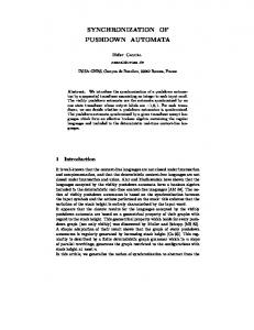
Fig. 7. Snapshot of vcg output for Tar-utility example.

Model checking our push-down model of the utility reveals that the policy is violated; all counter-examples are presented in a convenient tree-like layout as illustrated in Figure 7. The counter-examples indicate that the program reads files not specified 13

as an input argument; in particular, it requires access to dynamically loaded class files. Presentation of all counter-examples expedites recognition of this root cause of all violating paths in the system. After refining the policy to allow reading of class files, the model checker reports that the PDS model satisfies the refined policy. The second example is an ftp-server program for Linux, available from ftp.openbsd.org. Among other things, this program allows a remote user to execute commands such as ls and cd at the ftp server-site. Before doing so, however, the ftp-daemon must check that the user is authorized to issue these commands. This is accomplished by password-validation for which the ftp-daemon has to read from the /etc/passwd file. Once the user is successfully authenticated the ftp daemon establishes the uid for running such commands with setresuid. An interesting property to check therefore is: before issuing the system call setresuid there should be a call to open(/etc/passwd). We encoded the negation of this policy using the EFSA of Figure 6(b). The final state (p3 ) is reachable only when there is no open(etc/passwd) system call preceding setresuid. Model checking a finite-state model of the ftp program against this policy produced numerous counter-examples, closer inspection of which revealed that the violations occurred due to abstraction performed during model generation. The abstraction in question introduced non-deterministic branch points into the model; this resulted in infeasible paths which were the source of the counter-examples.

7 Related Work Related work in the areas of abstraction refinement and model checking of push-down systems has been discussed previously in Section 1. In other related work, [11] presents a technique where multiple counter-examples are used iteratively (one at a time) for refining an abstract system model. In [2, 13], the generation of counter-examples from the model checking of sequential-program models (control-flow graphs and labeled transition systems, respectively) is considered. The goal is to identify the root cause of error traces resulting from multiple executions of the model checker. In contrast to these approaches, our algorithm produces a succinct symbolic representation of all possible witness traces of a push-down system, and subsequently generates all minimum-recursion loop-free counter-examples from this data structure. Collective analysis of these counter examples may then be used to identify the common root cause of security-policy violations and to refine policies where appropriate. As emphasized in [15], the presentation of all possible counter-examples minimizes the number of model-checking runs required.

8 Discussion In this paper, we presented an algorithm that given a push-down model representing a sequential program with (recursive) procedure calls and an extended finite-state automaton representing (the negation of) a safety property, generates all minimumrecursion loop-free counter-examples. Our algorithm is also applicable, without modification, to finite-state system models. The utility of our techniques was illustrated via 14

application to a Java-Tar utility and an FTP-server program, and a prototype tool implementation offering a number of abstraction techniques for easy-viewing of generated counter-examples was discussed. As future work, we are exploring the use of machine-learning techniques to automatically identify commonality between counter-examples; the main idea is to recognize the longest common subsequence of action sequences on multiple counter-examples. Such pattern recognition enhances the usability of the tool. Another important avenue of research is to extend our techniques to the model checking of push-down systems for liveness properties. The major issue here is to define a finite representation for counterexamples and to extract such violating traces from model-checking results. Acknowledgements. The authors are grateful to the anonymous referees for their valuable comments on an earlier version of this paper.

References 1. R. Alur, T. Dang, and F. Ivanˇci´c. Counter-example guided predicate abstraction of hybrid systems. In International Conference on Tools and Algorithms for the Construction and Analysis of Systems, 2003. 2. T. Ball, M. Naik, and S.K. Rajamani. From symptom to cause: Localizing errors in counterexample traces. In Symposium on Principles of Programming Languages, 2003. 3. S. Basu, K.N. Kumar, R.L. Pokorny, and C.R. Ramakrishnan. Resource-constrained model checking for recursive programs. In International Conference on Tools and Algorithms for the Construction and Analysis of Systems, 2002. 4. A. Bouajjani, J. Esparza, and O. Maler. Reachability analysis of pushdown automata: Application to model checking. In Concurrency Theory, 1997. 5. E.M. Clarke, E.A. Emerson, and A.P. Sistla. Automatic verification of finite-state concurrent systems using temporal logic specifications. ACM Transactions on Programming Languages and Systems, 8(2), 1986. 6. E.M. Clarke, O. Grumberg, S. Jha, Y. Lu, and H. Veith. Counterexample-guided abstraction refinement. In 12th International Conference Computer Aided Verification, 2000. 7. S. Das and D.L. Dill. Counter-example based predicate discovery in predicate abstraction. In 4th International Conference on Formal Methods in Computer-Aided Design, 2002. 8. J. Esparza, D. Hansel, P. Rossmanith, and S. Schwoon. Efficient algorithms for model checking pushdown systems. In 12th International Conference Computer Aided Verification, pages 232–247. Springer-Verlag, 2000. 9. J. Esparza and S. Schwoon. A BDD-based model checker for recursive programs. In 13th International Conference Computer Aided Verification, pages 324–336. Springer-Verlag, 2001. 10. A. Finkel, B. Willems, and P. Wolper. A direct symbolic approach to model checking pushdown systems. In 2nd International Workshop on Verification of Infinite State System, volume 9. Elsevier Science, 1997. 11. M. Glusman, G. Kamhi, S. Mador-Haim, R. Fraer, and M. Y. Vardi. Multiple-counterexample guided iterative abstraction refinement: An industrial evaluation. In International Conference on Tools and Algorithms for the Construction and Analysis of Systems, 2003. 12. A. Groce, D. Peled, and M. Yannakakis. Adaptive model checking. In International Conference on Tools and Algorithms for the Construction and Analysis of Systems, 2002. 13. A. Groce and W. Visser. What went wrong: Explaining counterexamples. In SPIN Workshop, 2003.

15

14. H. R. Lewis and C. H. Papadimitriou. Elements of the Theory of Computation. Prentice Hall Inc., 1998. 15. K. Namjoshi. Certifying model checkers. In 13th International Conference Computer Aided Verification, 2001. 16. G. Pace, N. Halbwachs, and P. Raymond. Counter-example generation in symbolic abstract model-checking. In 6th International Workshop on Formal Methods for Industrial Critical Systems, Paris, 2001. Inria. 17. C. S. Pasareanu, M. B. Dwyer, and W. Visser. Finding feasible counter-examples when model checking abstracted Java programs. In International Conference on Tools and Algorithms for the Construction and Analysis of Systems, 2001. 18. J. P. Queille and J. Sifakis. Specification and verification of concurrent systems in Cesar. In International Symposium on Programming, volume 137 of LNCS, Berlin, 1982. SpringerVerlag. 19. H. Sa˝ıdi. Model checking guided abstraction and analysis. In Static Analysis Symposium, 2000. 20. G. Sander. Graph layout through the VCG tool. In Graph Drawing, DIMACS International Workshop, volume 894 of LNCS, pages 194–205, 1995. 21. R. Sekar, C.R. Ramakrishnan, I.V. Ramakrishnan, and S. A. Smolka. Model-carrying code: A new paradigm for mobile-code security. In New Security Paradigms Workshop, Cloudcroft, New Mexico, 2001. 22. XSB. The XSB logic programming system. Available from http://xsb.sourceforge.net.

16