GENERATION OF REPRESENTATIONS FOR ... - CiteSeerX

GENERATION OF REPRESENTATIONS FOR SUPERVISED LEARNING - A VELOCITY ESTIMATION EXAMPLE Magnus Borga, Mats Andersson and Hans Knutsson Department of Biomedical Engineering Link¨oping University Sweden {magnus, matsa}@imt.liu.se ABSTRACT A two-step learning method for velocity estimation is presented. First, an efficient representation of velocity is found using a learning technique based on canonical correlation analysis. This results in a spherical representation. Then, given this new representation, the mapping from input data to velocity estimates are learned by minimizing the mean square error between the output and the desired output on a training set. The non-linear mapping on the ’velocitysphere’ representation improves the performance of the linear method in the supervised learning step.

1. INTRODUCTION For high dimensional data, relevant feature extractors are in practice impossible to design by hand due to the overpowering amount off possible signal combinations. This particularly evident in problems involving images, image sequences and volumes where the dimensionality of the input data typically is in the range 105 − 108 . The situation is well exemplified by the medical field where new imaging techniques are consistently producing increasing amounts of data, e.g. high resolution CT and MR volumes and volume sequences. For this reason designing adaptive systems, comprising mechanisms for learning, appears to be the only possible route to attain a major improvement in system performance. An important step in image analysis is the estimation of certain features in images, volumes or sequences. When measuring a particular feature, e.g. local orientation or velocity, there are two important issues that has to be decided. The first issue is how the feature is to be represented. The importance of a good representation has been pointed out, e.g. in [7, 8, 11, 5] as well as by other authors. A good representation carries a maximum of information about the represented feature and it does so in a continuous way, suitable for further processing. Once a suitable representation has been chosen, the second issue is how to estimate the parameters for the given representation.

Both these issues can be dealt with by adaptive methods or learning techniques. It has previously been shown that canonical correlation analysis (CCA) can be used for finding efficient feature representations [4, 10]. The second issue of parameter estimation can be solved by supervised learning techniques, i.e. by minimizing an error between the estimated parameters and the desired estimates for a set of training examples. In the present work, we show how we can use a twostep learning approach for estimating velocity. First, CCA is used for finding a good representation of velocity. Then, given the new representation, the mapping from input data to this velocity representation are learned by minimizing the mean square error between the output and the desired output on a training set. In the following section is described how CCA can be used for learning feature representations. In section 3, an algorithm for estimation of velocity in the learned representation is presented. 2. USING CCA FOR LEARNING VELOCITY REPRESENTATION Canonical correlation analysis has previously been used for learning different kinds of representations [4, 10]. In this section, we first give a brief description of CCA. The velocity estimation involves a substantial amount of preprocessing and consists of feeding the input data through a quadrature filter bank. The implementation was done using a particularly efficient technique called convolver network that deserves a somewhat more detailed explanation in section 2.2 before the learning part is described in section 2.3. 2.1. Canonical correlation analysis Consider two random variables, x and y, from a multi-dimensional distribution:       x x0 Cxx Cxy ∼N , , (1) y y0 Cyx Cyy

where Cxx and Cyy are the nonsingular within-set covariance matrices and Cxy = CTyx is the between-sets covariance matrices. Consider the linear combinations, x = wxT (x − x0 ) and y = wyT (y − y0 ), of the two variables respectively. The correlation between x and y is given by equation 2, see for example [1]: wxT Cxy wy

ρ= q

wxT Cxx wx wyT Cyy wy

.

(2)

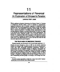
The maximum of ρ with respect to wx and wy is the largest canonical correlation. A complete description of the canonical correlations is given by:   −1     w ˆx ˆx [ 0 ] Cxy λx w Cxx [ 0 ] =ρ (3) Cyx [ 0 ] w ˆy λy w ˆy [ 0 ] Cyy ˆ indicates a where: ρ, λx , λy > 0 and λx λy = 1. w normalized vector, i.e. a vector of unit length. Equation 3 can be rewritten as:  C−1 ˆ y = ρλx w ˆx xx Cxy w (4) C−1 C w ˆy yx ˆ x = ρλy w yy ˆ xn , w ˆ yn }, n = Solving equation 4 gives N solutions {ρn , w {1..N }. N is the minimum of the input dimensionality and the output dimensionality. The linear combinations, xn = T T (x − x ¯) and yn = w ˆ yn (y − y ¯), are termed canonical w ˆ xn variates and the correlations, ρn , between these variates are termed the canonical correlations [6]. More details can be found in [1, 4]. 2.2. Convolver network Convolver networks is a new and efficient approach for optimization and implementation of filter banks [3]. The multi layered structure of a convolver network enable a powerful decomposition of complex filters into simple filter components. Compared to a direct implementation a convolver network uses only a fraction of the coefficients to provide the same result. The individual filters of the network contain very few coefficients. Figure 1 depicts the convolver network used for learning velocity representation. The nodes constitute summation points and the filters are located on the arcs connecting two consecutive layers. In figure 1 the filters are represented by plain arcs or by a circle containing a number of 3-5 dots. The dots correspond to both the number of nonzero coefficients in the filter and the position (coordinates) for these coefficients. The definition of the filter network can be divided into structure and internal properties. The structure of the network are the properties that can be read out from a sketch like in figure 1 i.e. the number of levels and the number of nodes on each level. The internal properties comprise the coordinates for the nonzero coefficients, the ideal filter function fm (u) and weight functions

~ f1

~ f2

~ f3

~ f4

~ f5

~ f6

~ f7

~ f8

~ f9

Fig. 1. Convolution network producing 8 quadrature filters spanning over 3 octaves using less than 150 real valued multiplications. Wm (u) for each output node, where u are Fourier domain coordinates. The filter coefficients cn in the network are computed to minimize the weighted difference between the resulting and the ideal filter functions. min 2 =

M   2 X

Wm (u) f˜m (u) − fm (u)

(5)

m=1

The Fourier weighting function W (u) provide an appropriate Fourier space metric. The choice of W (u) should if possible be done in the light of the expected spectra for the signal and the noise, see [9]. It is possible to optimize all filters on one level simultaneously with respect to the output filters and the current state of the network. This procedure is repeated for another layer and so on creating a sequential optimiser loop over the network structure by computing the partial derivatives. For more details see [3]. 2.2.1. A quadrature channel network The network in figure 1 corresponds to the the partitioning of the Fourier domain illustrated to the left in figure 2. The upper right branch in figure 1 consists of sequential 1D LPfilters. The centred squares in figure 2 illustrate the effect of this branch. Note that as this branch is traversed the distance between the coefficients are gradually increased i.e. the filters are becoming more sparse towards the lower levels. The eight first output nodes in figure 1 are broadband quadrature filters. These filters are computed pairwise where

f

Fig. 2. Partitioning of the Fourier domain. The figures cover the range [−π/2, π/2] in the FD. Left: Stylised scale/orientation patches. Constructed by a sequence of a 1/2 octave scale change and a coupled rotation of 45 degrees. This has a direct correspondence to the structure of the convolver network used. Right: Plot of 6dB limit of the resulting filters. The bandwidth of the filter vary from over 3 octaves for the high frequency filters to 2 octaves for the low frequency filters. The center frequencies are in the √ range [π/2 2, π/8].

CCA

f

Fig. 4. A symbolic illustration of the method of using CCA for finding feature detectors in images. The desired feature (orientation: here illustrated by a solid line) is varying equally in both image sequences while other features (here illustrated with dotted curves) vary in an uncorrelated way. The input to the CCA is a function f of the image.

v v

Fig. 5. Generation of training data. Fig. 3. Fourier domain magnitude of one of the eight quadrature filters produced by the convolver network. the relative direction of the filters differ by π/2. To the left in figure 2 one filter from each such pair are visualised by (somewhat overlapping) shaded areas. (The last output node is a real valued LP-filter which is not used for learning velocity but improves optimization convergence.) The network produces 8 quadrature filters using less than 150 real valued multiplications per pixel. Each quadrature filter is consequently obtained by the same effort as a direct implementation of a complex valued 3 × 3 filter. The right part of Figure 2 shows the 6dB limits of the resulting quadrature filters (and the LP-filter). Figure 3 shows the Fourier domain magnitude in detail of one of the eight quadrature filters produced by the convolver network. 2.3. Learning velocity representation The general principle behind the CCA-approach for learning representations is illustrated in figure 4.Two signals are fed into the CCA. The feature for which we want to find

a representation, e.g. velocity, is common in the two signals and therefore generate dependent signal components. The signal vectors fed into the CCA are image data mapped through a function f . If f is the identity operator (or any other full-rank linear function), the CCA finds the linear combinations of pixel data that have the highest correlation. In this case, the canonical correlation vectors can be seen as linear filters. In general, f can be any vector-valued function of the image data, or even different functions fx and fy , one for each signal space. The choice of f is of major importance as it determines the representation of input data for the canonical correlation analysis. In the case of learning a velocity representation, the basic idea is to feed filter output to the CCA in such a way that velocity is the only common information in the two inputs. Therefore the input is taken from two windows in an image. the windows are moving with the same velocity and in the same direction. This produces two sequences where the only common varying feature is the velocity. Each window consists of 9 points i a square grid as illustrated in figure 5. The offset between the windows was chosen randomly ev-

1

0.4

0.8

0.3

0.6

0.2

0.4

0.1

0.2

0

0 0

−0.1 50

100

150

−0.2

Fig. 6. Plot of the canonical correlations obtained in the velocity experiment.

−0.3 −0.4 −0.4

ery 500 step. The total training consisted of 5000 steps. The motion was defined by a vector that was randomly changed every step with a change of -1, 0 or 1 in each direction. The norm of the motion vector was limited to 5 (pixels per step). For each step, t, the convolver network produced 8 quadrature filter outputs for each of the nine points in the grid. The filter output was then multiplied by the conjugate of the corresponding filter output from the previous step: ∗ Qij (t) = qij (t)qij (t − 1)

−0.2

0

0.2

0.4

Fig. 7. Projections of velocity induced signals onto the first two canonical vectors. The true direction of velocity is indicated with an arrow. 0.5

(6)

where qij (t) is the output of filter i in position j at time t. Qij are called velocity channels. Quadrature filters give complex filter responses where the complex phase indicate if the signal under the filter is even (0 or π) or if it is odd (±π/2) or something in between. Because of the conjugate in equation 6, each velocity channel contain the phase difference between a filter output in one frame and the output of the same filter in the previous frame. Hence, the velocity channels contain information about the local velocity component in the direction of the corresponding filters. Since 8 filters are used, Qij (t) can be represented as 72-dimensional complex vectors. The velocity channel vectors are then normalized and divided into a real and an imaginary part. The result is pair of a 144-dimensional vectors from each window. This pair is then used as input to the CCA. The resulting canonical correlations are plotted in figure 6. The solid line shows the random correlation estimates for white Gaussian noise of the same dimensionality and the same number of samples. To visualise the resulting velocity representation, the filter response vectors for different velocities were projected onto the three most significant CCA-vectors. In figure 7, the projections onto the first two vectors are plotted and at each point, the true direction of velocity is indicated with an arrow. The clusters in the middle of the figure are caused by the quantization of the velocity in whole pixels per time unit. Figure 8 shows the projections onto the first and the third CCA-vector. Here, also the magnitude of the true ve-

0

−0.5 −0.5

0

0.5

Fig. 8. Projections of velocity induced signal onto the first and the third CCA-vector. The true velocity is indicated as arrows. locity is indicated as the length of the arrow. The reason for choosing only three vectors is that simplifies the geometrical interpretation of the solution. From figures 7 and 8 we see that the CCA has generated a three-dimensional representation of the velocity approximately on the surface of a bowl. In the first two dimensions, the direction is represented, while the magnitude of the velocity also uses the third dimension. A stylised version of the generated 3D representation is shown in figure 9. 3. SUPERVISED LEARNING FOR VELOCITY ESTIMATION This section presents an engineering approach to the results in the previous part of the paper. The algorithm is based on the velocity sphere representation and on the velocity chan-

v = oo

v=0

Fig. 9. A stylised version of the generated 3D representation of velocity. nels. The algorithm is efficient, robust and uses supervised learning in a training stage which makes it simple to adapt for different purposes.

other (two or three) parameter representation would imply that the estimation becomes more nonlinear which reduce the possibilities to preserve the motion information when using a linear estimation method. If a velocity estimate, µ, is not located on the sphere, the mapping in eq. 8 cannot be used directly. In this case the estimate must first be projected onto the sphere (maintaining the direction and the µ3 coordinate). A three parameter motion estimate consequently provide the means to form an opinion about the confidence of the estimate. Velocity estimates located at a distance from the ideal surface in the 3D parameter space imply that either the local neighbourhood or the motion does not fit the applied model and the estimated velocity should be treated with great care. This feature is extremely important for a robust motion estimation and is by itself a sufficient motivation for using the velocity sphere representation.

3.1. Velocity sphere representation A three parameter representation of the velocity that corresponds to figure 9 is obtained as follows. Let v = (vx , vy )T denote the velocity in a neighbourhood of an image sequence. The new representation µ = (µ1 , µ2 , µ3 )T is computed as   θv = 2 tan−1 kvk v0 µ1 µ2 µ3

= vx sin(θv )kvk−1 = vy sin(θv ) kvk−1 = − cos(θv )

(7)

The parameter v0 corresponds to an expected average velocity and is mapped to the equator of the velocity sphere. Considerably smaller or larger values of v0 will concentrate the contributions towards either of the poles and the purpose of the mapping will be lost. What is the advantage of estimating the three parameter representation of the velocity as opposed to estimate (vx , vy ) directly? The canonical correlation finds more information using this representation but it does not explicitly explain why. The velocity sphere representation in eq. 7 is not a final result but an intermediate step between the velocity channels and a (vx , vy ) estimate. Consider for the moment a velocity estimate, µ, that is located on the sphere in figure 9. The mapping from this representation to the conventional velocity representation is given by kvk vx

= v0 tan(0.5 cos−1 (−µ3 )) = kvk √ µ21 2

vy

= kvk √

µ1 +µ2 µ2 µ21 +µ22

(8)

Note that the nonlinearities in eq. 8 are not a part of the estimation process as would be the case if (vx , vy ) were to be estimated directly from the velocity channels. The canonical correlation states that a representation like in eq. 7 is the most efficient three parameter representation for preserving the motion information of the velocity channels. Using any

3.2. Velocity channels The quadrature filter responses from the convolver network in figure 1 is denoted q = (q1 , q2 , . . . , q8 )T . From these eight filter responses 24 velocity channels are computed where each filter contribute to three channels. Qnm (x, t)

= qn (x − dnm , t − 1) qn∗ (x, t)+ qn (x, t) qn∗ (x + dnm , t + 1)

(9)

The definition of these velocity channels differ in two aspects from the previous one used in the canonical correlation step (eq. 6). These channels are computed over three temporal coordinates instead of two. Apart from an increased temporal support this approach preserves the (temporal) sampling grid. The second difference is that a spatial offset vector dnm m ∈ [1, 2, 3] is introduced where dn2 = 0 and dn1 = −dn3

(10)

The magnitude of the nonzero offset vectors is proportional to the spatial √ extent of the quadrature filter and varies from kd11 k = 2 for the high frequency filters to kd81 k = 7 for the low frequency filters. The direction of dnm coincide with the direction of qn , see figure 2. The introduction of the offset vector is simply a method to increase the spatial resolution of the velocity estimate at the expense of an increased number of velocity channels. Consider for example the velocity channels originating from a quadrature filter along the x-axis where the magnitude of the non zero offset vector kdk = 3. The phase and magnitude of these velocity channels probe the possibilities that the neighbourhood is moving to the left by 3 pixels/frame, no motion is present and motion to the right by 3 pixels/frame. If the actual motion corresponds exactly to one of these hypotheses we obtain a high magnitude and zero phase for this velocity channel. The magnitude of Qmn works mainly as a confidence measure while the argument provides continuous velocity estimation in relation to the

intrinsic velocity of the channel (the offset vector dmn ). The velocity channel approach can be described in terms of correlation but in difference to conventional correlation where the intensity values of the original image is used, the phase of the velocity channels support sub-pixel accuracy at a fraction of the computational effort. The velocity channels are computed for every neighbourhood in the sequence and represented as a vectors. These complex valued 24-dimensional Q-vectors are normalized and then divided into real and imaginary parts. The velocity channels are finally represented as real valued 48dimensional vectors. 3.3. Training of the velocity estimation

Fig. 10. The first frame (out of 12) in the training sequence. The frames are interlaced and the maximal velocity is 12 pixels/frame.

Fig. 11. Spatial weight, sw (x), used for all frames in the supervised training. The velocity channel responses constitute a high dimensional description of both the spatial properties as well as the motion in the local neighbourhood. The purpose of this section is to map this high dimensional description to the

Fig. 12. The magnitude of the estimated velocity for a frame in the test sequence.

Fig. 13. The magnitude of the error for a frame in the training sequence. The unweighted error is 1.60 pixels/frame and the weighted error is 0.97 pixels/frame. The peak velocity in the test image is 12 pixels/frame.

selected three parameter representation of the local velocity. To directly formulate such a mapping is cumbersome. A more interesting method is to compute the mapping using supervised learning. A training image sequence is produced, where the three parameter representation of the velocity, µ(x, t), is known for each spatial position, x, and frame, t, in the sequence. A frame from the training sequence is shown in figure 10. The total length is 12 frames which complete one period. The high frequency sectors move inwards and the low frequency sectors move outwards. In the central part no motion is present. The maximal velocity is 12 pixels/frame and the training sequence is (as most video sequences) interlaced. The purpose of the training is to find the 48 × 3 weight matrix, W , that minimize the error in the training sequence according to eq. 11. min 2 =

X


sw (x, t) µ(x, t) − W T Q(x, t) 2 (11) x,t

The spatiotemporal weight, sw (x, t) is a scalar that controls the importance of a close fit in position (x, t) of the training sequence, see figure 11. Generally sw (x, t) is used to emphasize the accuracy for the areas in the training sequence that contain low or zero velocities. By computing ∂2 ∂W

(12)

and setting the partial derivative equal to zero the weight matrix is obtained as #−1 " X X 2 T sw Q Q s2w Q µT (13) W = x,t

x,t

which complete the training phase. To produce a training sequence is a delicate task. It is important that the velocity in the training sequence is uncorrelated to as many features as possible (orientation, spatial frequency, phase, SNR, etc). In addition to this the training should focus on events that is of certain importance for the considered application e.g. a robust behaviour in the presence of multiple motions. The proposed velocity estimation algorithm can now be expressed as: 1. Compute the quadrature filter responses using the convolver network in figure 1. 2. Compute the velocity channels in eq. 9. 3. Compute the three parameter velocity representation originating from the canonical correlation analysis as µ = W T Q. 4. Compute the conventional velocity estimate (vx , vy ) using eq. 8. Figure 12 show the magnitude of the estimated velocity for a frame of the training sequence. The overall unweighted error is uw = 1.60 pixels/frame and the weighted error w = 0.97 pixels/frame. The weighted error is computed using the same spatial weight, sw , that were used in the training. In figure 13 the magnitude of the error is shown. 4. CONCLUSION We have shown how a two-step learning approach can be used for estimating velocity. First, an efficient representation of velocity was found using a learning technique based on canonical correlation analysis. Given this new representation, the mapping from input data to velocity estimates was then learned by minimising the mean square error between the output and the desired output on a training set. To evaluate the performance of an algorithm for velocity estimation is cumbersome. Most algorithms are designed or tuned to perform extremely well when the motion is limited to 1-2 pixel/frame and consists of a pure translation.

A robust behaviour for large velocities and in the presence of multiple motions is often not addressed. A solid evaluation of different motion estimation algorithms can, however, be established by using the algorithms as a motion compensated predictor in a video coder and simply measure the transmitted bit rate. The proposed algorithm is used as an efficient and robust motion estimator for a video coder in [2] with very good results. 5. DISCUSSION In the supervised learning step, we did not use exactly the representation found by the CCA method. Instead a simplified and idealised handmade representation was used, which had the same basic properties as the representation generated by the CCA method. First, the simplification was made that only the three strongest canonical correlations were used. Then the noisy and quantized appearance of a sphere was replaced by an ideal sphere. The first step, to use only the three strongest canonical correlations, means that some information was not used. On the other hand, the second step of replacing the noisy and quantized appearance of a sphere by an ideal sphere is likely to have improved performance, since the the quantization and probably also the noise is caused by the training data. Further investigations will show if the full use of the actual representation generated by the CCA method will further improve performance. The major point here is that CCA can be used to find a non-trivial representation for image features and that this representation can be used in further processing. 6. REFERENCES [1] T. W. Anderson. An Introduction to Multivariate Statistical Analysis. John Wiley & Sons, second edition, 1984. [2] K. Andersson, M. Andersson, and H. Knutsson. A perception based velocity estimator and its use for motion compensated prediction. In Proceedings of the 12th Scandinavian Conference on Image Analysis, Bergen, Norway, June 2001. [3] M. Andersson, J. Wiklund, and H. Knutsson. Filter Networks. In Proceedings of Signal and Image Processing (SIP’99), Nassau, Bahamas, October 1999. IASTED. Also as Technical Report LiTH-ISY-R2245. [4] M. Borga. Learning Multidimensional Signal Processing. PhD thesis, Link¨oping University, Sweden, SE581 83 Link¨oping, Sweden, 1998. Dissertation No 531, ISBN 91-7219-202-X.

[5] G. H. Granlund and H. Knutsson. Signal Processing for Computer Vision. Kluwer Academic Publishers, 1995. ISBN 0-7923-9530-1. [6] H. Hotelling. Relations between two sets of variates. Biometrika, 28:321–377, 1936. [7] H. Knutsson. Producing a Continuous and Distance Preserving 5-D Vector Representation of 3-D Orientation. In IEEE Computer Society Workshop on Computer Architecture for Pattern Analysis and Image Database Management - CAPAIDM, pages 175–182, Miami Beach, Florida, November 1985. IEEE. Report LiTH–ISY–I–0843, Link¨oping University, Sweden, 1986. [8] H. Knutsson. Representing Local Structure Using Tensors. In The 6th Scandinavian Conference on Image Analysis, pages 244–251, Oulu, Finland, June 1989. Report LiTH–ISY–I–1019, Computer Vision Laboratory, Link¨oping University, Sweden, 1989. [9] H. Knutsson, M. Andersson, and J. Wiklund. Advanced Filter Design. In Proceedings of the Scandinavian Conference on Image analysis, Greenland, June 1999. SCIA. Also as report LiTH-ISY-R-2142. [10] Hans Knutsson and Magnus Borga. Learning Visual Operators from Examples: A New Paradigm in Image Processing. In Proceedings of the 10th International Conference on Image Analysis and Processing (ICIAP’99), Venice, Italy, September 1999. IAPR. Invited Paper. [11] C-F. Westin. A Tensor Framework for Multidimensional Signal Processing. PhD thesis, Link¨oping University, Sweden, SE-581 83 Link¨oping, Sweden, 1994. Dissertation No 348, ISBN 91-7871-421-4.