(pseudo) electrons. To do so we' need to understand how a pseudopotential can be defined from the all-electron wave function. The response of an atom to a ...
Generation
of pseudopotentials
from correlated
wave functions
Paula H. Acioli Physics Department, University of Illinois at Urbana-Champaign,
Urbana, Illinois 61801
David M. Ceperley National Center for Supercomputing Applications, and Physics Department, University of Illinois at Urbana-Champaign, Urbana, Illinois 61801
(Received 13 December 1993; accepted 15 February 1994) The density matrix, or equivalently the natural orbitals play an essential role in transferability of pseudopotentials to all orders of perturbation theory. In this work density matrix and natural orbitals of Li, C, and Ne atoms are obtained using diffusion Monte Carlo. Using these a pseudopotential is computed for the lithium
I. INTRODUCTION Accurate ab initio calculations of the electronic properties of solids and molecules with heavy atoms require good pseudopotentials. Treating heavy atoms is especially difficult because chemically interesting energies are only a small fraction of the total energy. Quantities such as the binding energy depend mostly on the properties of the valence electrons, but the core electrons have the largest contributions to the total energy. Hence it is very useful (or practically necessary) to separate the core and valence electrons and replace the core degrees of freedom with a pseudopotential. The pseudopotential describes the interactions of the valence electrons with core (nucleus plus core electrons), as well as the Pauli exclusion principle between the valence and core electrons. The generation of pseudopotentials in one-particle theories, such as Hartree-Fock @IF) or density functional theory (DFT), is a well-understood problem because there is one-toone correspondence between the potentials and the oneparticle spectrum. Norm conserving pseudopotentials1-6 take full advantage of this correspondence to reproduce the scattering properties of the valence electrons. The problem with the one-particle theories is that correlation effects, when included, are included in an approximate manner, such as in the local density approximation (LDA). Because the valence properties depend strongly on correlation effects it is very important to include them more accurately in the pseudopotential. Shirley and Martin7 have used a generalized GW method to compute the effects of core polarization, which correct a Hartree-Fock treatment of the core-valence interactions. Core polarization has also been considered by Miiller et aZ.* for treatment of intershell correlation effects for the use in ab initio self-consistent field (SCF) and configuration interaction (CI) calculations. We suggest, in this paper, how to use quantum Monte Carlo methods (QMC) to generate pseudopotentials, from the exact many-body wave function. These pseudopotentials can then be used in QMC simulations of the valence only (pseudo) electrons. To do so we’need to understand how a pseudopotential can be defined from the all-electron wave function. The response of an atom to a weak external perturbation can be computed from its density matrix, thus it is important to ensure the density matrices are unchanged when J. Chem. Phys. 100 (ll),
1 June 1994
0021-9606/94/i
determining the the one-particle variational and atom.
the core electrons are removed. This leads to a natural definition of a pseudopotential. Of course these density matrices~ can be computed by any quantum chemistry method. It is somewhat surprising that 60 years after the birth of quantum mechanics and 40 years after the relevance of density matrices to quantum chemistry was pointed out by Lowdin,‘* that accurate tables of atomic natural orbitals (including relativistic effects) for all the elements are not available. In this work we compute the one-body density matrix and natural orbitals for the atoms of lithium, carbon, and neon, using QMC. We then show how one can generate pseudopotentials based on the one-body density matrix. We generate the pseudopotentials of lithium using its natural orbitals and compare with the same kind of calculation using the natural orbitals obtained from a CI calculation.g In Sec. II we will review some of the properties of density matrices and natural orbitals. In Sec. III we discuss the generalization of the norm-conservation pseudopotentials to many-body wave functions. In Sec. IV we discuss the basics of QMC and show how to compute the one-body density matrix with QMC. In Sec. V we present the natural orbitals and pseudopotentials we computed in this work. We then give the main conclusions of this work and the prospects of future work.
II. DENSITY MATRIX In Sec. III we will consider the interaction of two arbitrary atoms, A and B. We then replace atom A (which contains all of its electrons), with a pseudoatom A containing only valence electrons. How should the wave functions be truncated so that the atom and pseudoatom appear identical to B? In quantum statistical mechanics, one introduces the density matrix to simplify the division of the universe into two parts.‘o So it is not surprising that the properties of a pseudopotential should be determined by the density matrix of an isolated atom. The p-particle matrix is defined” in terms of the wave function p( r t , . . . , rN) of a N-particle system:
00(11)/8169/9/$6.00
0 1994 American Institute of Physics
8169
Downloaded 28 Apr 2003 to 130.126.9.235. Redistribution subject to AIP license or copyright, see http://ojps.aip.org/jcpo/jcpcr.jsp
P. H. Acioli and D. Ceperley: Pseudopotentials
8170
dP)(rl,r2 ZZ x*(r;
III. GENERALIZATION
,..., rP.plri ,ri ,..., r;) drp+&+2
---dr,**(rl,r2
,..., rP ,..., rN)
,ri ,..., r; ,... 4-N).
(1)
For a system at finite temperature, one must also sum over a thermal occupation of states including different ionization states. For open shell atoms, it may be important to consider the electron spin when defining the density matrix. For a system, weakly interacting with its surroundings, the matrix element of the interaction potential can be written in an expansion of density matrices of different orders, as discussed below. In such an expansion the lower the order of the density matrix the more important is its contribution. So, the most important contribution comes from the one-body density matrix:
dr,r’> =N
I
dr2dr3 ~--dr$P*(r,r2,r3~--rN)‘P(r’,r2,r3~-~r~). (2)
We can write this symmetric matrix in terms of its eigenvalues and eigenfunctions. They are, respectively, the occupation numbers, ni, and the natural orbitals tii(r): (3)
The occupation numbers satisfy the inequality OGn$2 if the wave function has same spatial dependance for spin up and down electrons. For a Hartree-Fock wave function the natural orbitals are the same as the Hartree-Fock orbitals and have occupation number 0, 1, or 2 (unoccupied, single, or double occupancy). Thus the above definition is a very “natural” generalization of the concept of orbitals to manybody wave functions. The natural orbitals have a special significance in quantum chemistry because an expansion of the exact wave function in terms of determinants (CI) converges quickest in a natural orbital basis. Since an atom has spherical symmetry, the one-body density matrix can only depend on the three variables r. T’, and rer’. Note that when we write an atomic density matrix, we implicitly take the position of the ion as the origin of the coordinate system. The density matrix can then be expanded in angular momentum components 21+ 1
p(d)
= C
F
from correlated wave functions
OF NORM CONSERVATION
The main goal of a pseudopotential is to reproduce the response of an atom to an external perturbation, which can be either an external field, an electron, or other atoms. By this is meant that the perturbed “pseudoatom” energy levels are the same as in the full atom. This property is known as “transferability.” In this section we discuss the problem of generating pseudopotentials from many-body wave functions. To better understand such generalization we will first discuss norm-conserving pseudopotentials. In one-particle theories, where a one-electron Schrodinger equation is solved, the properties of the one-electron valence wave functions are approximately reproduced with a norm-conserving pseudopotential’ which is constructed as follows. (1) All-electron atom and pseudoatom energies agree for a chosen atomic configuration. (2) All-electron and pseudoatom (normalized) orbitals agree beyond a chosen “core radius,” r, . These two properties also imply that (3) The integrals from 0 to r of the all-electron and pseudocharge densities agree for T>T, for each valence state (norm conservation). (4) For some range of energies of a scattering electron, the atom and pseudoatom give the same total energy. One generalization of norm conservation to many-body wave function is to demand that the one-body density matrix of the all electron and pseudoatoms agree beyond the “core radius:” p(r,r’)=F(r,r’)
for r,r’>rcr
(6)
where p and fi are the one-body density matrices of the allelectron and pseudoatoms, respectively. This is completely equivalent to the norm-conservation concept for a oneelectron theory, since if condition (2) is satisfied its density matrix will also satisfy Eq. (6) and vice versa. Condition (1) still must be applied in the construction of the pseudopotential. To justify the above generalization we go to perturbation theory. Consider, for instance, a diatomic molecule formed by atoms A and B, with NA and NB electrons, and Hamiltonian:
H=H,+H,+C+-
ZAZB rAB
(7)
.
Pl(r,r’)lPl(i-~‘),
1
In the following we assume the atom A is at the origin and atom B is at RB . We have split H into “unperturbed” atomic Hamiltonians and an interaction piece:
where dap(r,r’)Pl(P.?).
(5)
Then the natural orbitals, eli( r) Y,,(a) are labeled by angular momentum, (Z,m) , and by level i. The definition of natural orbitals and occupation numbers can be extended to higher particle density matrices, but we will not use them in this paper.
“=Fb
&-Ix a
2-x a
2.
(8)
b
Let us now do perturbation theory starting from the basis of isolated atoms states:
J. Chem. Phys., Vol. 100, No. 11, 1 June 1994
Downloaded 28 Apr 2003 to 130.126.9.235. Redistribution subject to AIP license or copyright, see http://ojps.aip.org/jcpo/jcpcr.jsp
P. H. Acioli and D. Ceperley:
Pseudopotentials
=.ADpAa(q ,..-,rN~)~8P(rNA,~-RB,...,rN*~N~-RB), (9) where 02 and @)Bp are complete sets of exact solutions of HA and HB , respectively, and J&X,( - l)‘@ is a projection operator that antisymmetrizes the wave function in all NA + NB electron coordinates by summing over all ways of exchanging electrons between the two atoms. Perturbation theory using this basis will be quickly convergent as long as the cores do not overlap. Here we are assuming that the number of electrons on atoms A and B are fixed. If an electron is transferred from one atom to another, one must consider a more general basis and that will complicate the notation, but not introduce any essential complications. Consider the first-order expression of the ground state energy z*z,
EF)=E;+E;+-
+ (YOOI vpoo>
RB
(10)
-
from correlated wave functions
upper bound to the exact energy. It is not hard to see that the matrix element in the denominator can be expanded in terms of number of “exchanging” electrons in the antisymmetrization operator. The matrix element arising from p electrons simultaneously exchanging can then be related to the p-particle density matrix”
(TOOpOO) =l-
I
1 +fzy
dr$r:
I
drldr2dr;dr~p~(rl
,r2;r; ,r$
Xp~(r;-RRs,r~-RB;rl-RB,r2-RB)+~p~P~), (11) where pPAand p” are the p-particle density matrices for atoms The potential matrix element, the numerator of Eq. (lo), can be expanded in exactly the same way
’ PB(r,--&3-l--&)+
I
drldr~p~(rl;r~)p~(r~-RB;rl-RB)
A and B, respectively.
Note that this equation is valid for the nonorthogonal basis set we are using and the first-order perturbation energy is an
+
8171
?
pi(r:
;rl)pA(r:-RR,;rl--RB)+
I
&dr;
I drldr;
$
,
~p~(r,;rj)~~(r,-R,;r:-R,)
p~(r,;rl)p~(r;--RB;r;-RB) (12)
I
If the pseudoatom is to respond exactly as the full atom, every term in Bqs. (11) and (12) must be the same. Thus transferability is precisely the property that the full-atom and pseudoatom density matrices be identical. The separation into core and valence electrons occurs if we assume the electrons of atom B remain outside the core region of A. Expand the density matrices in terms of their natural orbitals. We find for the normalization integral in Eq. (11) (only up to single exchanges) that (JEoopPoo)= 1-c
nA,n~lM,p(R~>12+~p~p~),
(13)
a@
pseudopotential approximation consists of neglecting the contribution of core-core interaction and valence-core interaction. But in constructing the pseudo-orbitals it is important to keep all contributions which extend out of the core. Hence we are lead to Eq. (6). To demonstrate that the expansion in density matrices converges in the expansion of exchanging electrons let us recall the asymptotic behavior of atomic wave functions as a single electron is removed13 lim @(rr,rz ,..., rN)=&(rs r*-w
,...) rN)rf
exp(-err), (1%
where Ma8 is defined as ~W~"(r)@r+Rd.
04)
Considering atom B could be anything, and thus G(r) is arbitrary but confined to the valence region of A, we want the pseudo-orbitals to be the same as the full orbitals in the spatial region that of A can contribute to M. This demonstrates that it is only the occupied orbitals that matter and that valence orbitals contribute the most strongly. The
is the where CY= &,/3 = llcr - 1, and E=EN-~-EN first ionization potential. Then a p-particle density matrix will contain an exponential piece exp[ - a(rl -k -** -t ri)] where all of the 2p arguments of the density matrix are being pulled off the atom. Now assuming that R, is large (at least large enough so that the above expression for Q, is correct for r t > RB/2) then one can see that the maximum value of the overlap integrand occurs at the middle of the bond (assuming
a symmetricmoleculefor the moment)and that an exchange
J. Chem. Phys., Vol. 100, No. license 11, 1 June 1994 Downloaded 28 Apr 2003 to 130.126.9.235. Redistribution subject to AIP or copyright, see http://ojps.aip.org/jcpo/jcpcr.jsp
8172
P. H. Acioli and D. Ceperley:
Pseudopotentials
of p electrons will be reduced in value by a factor exp( - 2p LYRE); this is the convergence parameter of the expansion in Eqs. (11) and (12). So if we want to construct a pseudopotential for atom A and keep the integral in Eq. (11) unaltered, we just have to impose that outside the core the one-body density matrix for the pseudoatom is the same as the one-body density matrix of the real atom A. This is precisely the condition stated in Eq. (6). We can see that higher order density matrices will also enter in Eq. (1 1), but since they correspond to exchanges of more than one-electron they will be contributions of smaller order, and can be neglected in a first approximation. In fact, the effect of higher order exchanges is not neglected. We are constructing the pseudoatom based on the one-body density matrix and hope that the higher order pseudodensity matrices are close to their exact counterparts so that the contribution of the higher order density matrices also match. We restricted our analysis to first order in perturbation theory. At higher orders the corrections to the energy involve the overlap integral between two different states as well as the matrix elements of the interaction potential involving different states. These integrals can also be expanded in terms of the density matrices of the individual atoms of different orders. See Ref. 12 for detailed expressions. But the leading correction will always depend on the one-body density matrix of atom A. So, Eq. (6) guarantees that, for all orders in perturbation theory, the contributions coming from the onebody density matrix of atom A, which are the largest, will be correct, thus making the pseudopotential transferable. There are new terms such as those representing the polarizability of the ionic core. An accurate description of the atom might need to include such effects as well as relativistic effects on the core. But we will not discuss them in this paper. A possible procedure to generate correlated pseudopotentials is as follows.
from correlated wave functions
Car10’~ the expectation value of the Hamiltonian with respect to a trial wave function is computed with the Metropolis algorithm.15 The statistical average of the local energy EL= HqPP is an upper bound to the exact ground state energy (16) where ZI’is the trial wave function and R is sampled from
PI”.
In diffusion Monte Car10,‘~ one starts with the S&r& dinger equation in imaginary time: -y
-[-DV2+V(R)-&IQ)(R)
with D=A2/2m, and ET ,(the trial energy) a constant adjusted to keep the normalization of Q stationary. This can be thought as a diffusion equation in 3 N dimensions, and can be readily simulated. We use importance sampling by multiplying this equation by q (a trial function) and defining a new distribution f(R,t)=Q(R,t)W(R). Equation (17) becomes --
Jf (RJ) dt
=-DV2f(R,t)+[E,(R)-Er]f(R,t) 18)
where EL is the local energy; ET, is the trial energy; and F=V ln]!J!12.This is now a diffusion equation with branching and drift terms. Because the product @(R,t)q(R) is not gu& anteed to be always positive the random walks are restricted to regions of the same sign, this is what is called the fixed-nodeI approximation. Further details are given in Ref. 16. In this work we will use diffusion Monte Carlo to compute the one-body density matrix for Li, C, and Ne.
(1) Perform a many-body calculation for the all-electron atom, and compute the density matrix and natural orbitB. Wave function (2) groose a form for the pseudopotential with adjustable parameters. (3) For a chosen set of parameters, perform the same manybody calculation for the pseudoatom, and compute the density matrix and natural orbitals for the pseudoatom (4) Compare the occupied natural orbitals of the pseudoand all electron atoms. If they agree in the valence region, the pseudopotential satisfies the generalized normconserving criteria. If they do not agree, choose a new set of parameters and repeat step (3). We have only carried out this scheme for the Li atom. Since it has only a single valence electron, steps 2-4 are trivial. We have proposed this scheme with quantum Monte Carlo in mind, but it can be used with any many-body theory. IV. COMPUTATION A. Quantum
OF THE NATURAL ORBITALS
~~The wave function we used in our calculation, which includes both two- and three-body correlations, was first suggested by Boys and Handy.‘8*1g The actual form we use is from the work of Schmidt and Moskowitz2’
Wq,r2,...,
u9>
rN)=dett~)dett.t)exp
where UIij is a correlation polynomial. term form from Ref. 20
We used the nine
where r i&---il+br’
-~
.
(21)
Monte Carlo
In this section we ‘will briefly describe the variational and diffusion Monte Carlo methods. In variational Monte
S(y)=cly+C2y2+C3y3+Cqy4,
o-2)
P(,9=c5y2+c,5y3+c7,74
(23
J. Chem. Phys., Vol. 100, No. 11, 1 June 1994 Downloaded 28 Apr 2003 to 130.126.9.235. Redistribution subject to AIP license or copyright, see http://ojps.aip.org/jcpo/jcpcr.jsp
P. H. Acioli and D. Ceperley:
Pseudopotentials
and det(T)det(J.) are Slater determinant for spin up and down, respectively. For the determinants we use the SCF solution from Clementi and Roetti.21 C. Computation
of the one-body
density
matrix
The one-body density matrix has been calculated very often in liquid and solid hel.ium22*23since its Fourier transform is the momentum distribution and a key quantity is the fraction of atoms with zero momentum. Recently Lewart et a1.24extended these calculations to liquid helium (3He or 4He) droplets. We have followed their procedures except that we sampled the new point r’ instead of using a fixed grid and we performed the averages with diffusion Monte Carlo (DMC), instead of variational MC (VMC). First let us rewrite the density matrix as an expectation value over a random walk. The following notation will be useful: R=(rl,r2 ,..., rN) and R’ = (r; ,r2 ,..., q,). By rearranging the q’s in the definition of pl we get dri dR mW(R)
jY’(R)12PI(&
.;;)
6(r1 -r>qr;-r’)
X
(24)
(rr’)2
the integral over dR is done with either VMC or DMC. We introduce an additional sampling function g(r;) to perform the integration over dr; . At each step of the VMC run, the r; is sampled from g(r;) and the angles are sampled uniformIy over a sphere. The estimator of our density matrix in VMC is then N
8173
p$i=nifJi.
(30)
This direct method is exact in the limit of good statistics, and Ar-+O. Because of the statistical noise it is best to use smooth basis functions to reduce the noise in the resulting natural orbitals. When we use a basis set we transform the density matrix from the mesh to a new (smaller) matrix, that is also numerically diagonalized. We tested Gaussian’ and Slate?’ basis sets and found that the results are independent of the basis type. The most serious problems concern their behavior at large distances from the atom, where Gaussians decay too quickly. Since these basis are nonorthogonal, one has a generalized eigenvalue problem to solve. We now discuss the effect of statistical noise on the construction of the natural &bitals frbm the Monte Carlo estimated density matrix. First of all we symmetrize the variational estimator of p since any antisymmetric component is pure noise. Note that the “extrapolated” estimate (discussed below) will also be symmetrized. Upon calculating the occupation numbers, because of the statistical errors in the p(r,r’), one finds many that are small and negative. These were also found in the study of helium droplets by Lewart. The orbitals with small occupation number are very noisy. To test the correctness of our numerical methods we computed the natural orbitals of a HF wave function and compared the results with the original HF orbitals. They agreed with each other up to r=6 a.u. Obtaining the NO for pairs of states with the same angular momentum and the same occupation number (e.g., 1s and 2s of C and Ne) was a problem because they tend to mix. To separate them, we considered a linear combination
W(R’)S(ri-r)S(rl-r’)PI(~~.~‘)
pyb-,e=c i
from correlated wave functions
i
WRM-‘>W)2
) *
(25) The sum over particles can be performed because all electrons are identical. Note that we are ignoring the spin of the electron. We chose the sampling function so the errors on p would be roughly independent of r’
dzi +)=.jjzgg.
(26)
Here p(r) is the electronic density, the optimization of g has not been studied. For each I component we store the density matrix in a radial 100X 100 mesh. This matrix can be diagonalized directly if we think of the eigenvalue problem as
I dr r2pl(r,r’>~lii(r)=nli~lli(r’).
(27)
We convert this integral to a sum, multiply both sides by rk , and define Pjk=rjPl(rj
4j=j=j*drj)3
,rk)rkAr,
(2% .
(2%
where Ar is the radial grid spacing. We get the following eigenvalue problem, to be solved numerically:
where g is the number of degenerate eigenvalues. We then maximize $e “core” charge of the 1 s orbital ol =/:I
sl(r)]r2dr
(32)
with the constraint that the orbitals remain orthonormal. This procedure makes sense,in terms of pseudopotentials, since we would like to eliminate the most tightly bound electrons when constructing a pseudopotential but leave the valence charge unaffected. With this we are ensuring, as far as possible, that the core orbitals drop to zero rapidly outside the core. All the results presented in this paper used the above procedure to separate degenerate natural orbitals. We have also computed the density matrix with diffusion Monte Carlo which samples @P instead of I’P12,where Cpis the ground state wave function in the fixed node approximation. I6 The mixed density matrix is defined as ptix(rl,ri)=N
I
dr, dr,*-.dr,
q(R’)Q>*(R).
(33)
From last equation we can see that the form of the mixed estimator is similar to Eq. (2), the only difference is that we are now sampling a different distribution. Equation (33) is not symmetric under interchange of r and Y’ and the error is
J. Chem. Phys., Vol. 100, No.license 11, 1 June 1994 Downloaded 28 Apr 2003 to 130.126.9.235. Redistribution subject to AIP or copyright, see http://ojps.aip.org/jcpo/jcpcr.jsp
P. H. Acioli and D. Ceperley:
8174
Pseudopotentials
from correlated wave functions
TABLE I. Total energies of Li, C, and Ne. The HF energies are the ones from the work of Clementi and Roetti; the VMC, are the variational energies obtained by Schmidt and Moskowitz; DMC are the energies we obtained using the Diffusion Monte Carlo method, For the exact energies, we use the estimation of the correlation energies Veillard and Clementi (Ref. 29). Hartree-Fock Li C Ne
-1.4321 -37.6886 -128.547 1
VMC
DMC
Exact
-7.4731(6) -37.7956(7) -128.8771(5)
-7.4770(3) 737.8120(S) -128.9274(65)
-7.4781 -37.8451 -128.9370
0.75
0.25
of the order of A=@--*. We used the following “extrapolated” estimator which is symmetric and has an error of the order of A2 as discussed by Ceperley and Kalo~.~’ 2.0
-(pl(r,r’))‘“+@A2).
/
4.0
0
(34)
When the trial wave function is accurate, both the mixed and the extrapolated estimators will agree. But the extrapolated density matrix (and hence natural orbitals) is expected to be closer to the exact density matrix because one has removed the highest order errors of the trial function. The difference is an estimate of the systematic errors coming from the trial function. D. Computation
r (a.u.)
of the pseudopotential
If only a single electron remains in the valence shell it is straightforward to compute the pseudopotentials having the correct natural orbitals by inverting the Schrodinger equation. There remains the problem of how to extend the pseudopotential into the core region. We have used the scheme proposed by Kerker.26 The valence pseudo-orbital is assumed to have the following form: (35) where (Y, p, y, and S are chosen such that the normconserving conditions [conditions (l)-(4) in Sec. III] are satisfied. We computed the 1=O,l atomic pseudopotentials of lithium, using the 2s and 2p natural orbitals obtained from DMC runs. We did the same thing with the 2s and 2p natural orbitals computed on a CI calculation by Widmark et a1.,9 ,using the same energy eigenvalues for both cases. The results and further details are discussed in Sec. V. V. RESULTS Table I shows the total energies from our diffusion Monte Carlo runs, compared to those obtained by Schmidt and Moskowitz.20 We can see that DMC recovered 98% of the correlation energy of lithium, 79% of carbon, and 98% for neon, compared to 89%, 68%, and 85% obtained by Schmidt and Moskowitz with VMC. We might then anticipate that the NO obtained with diffusion Monte Carlo will be more accurate than the ones obtained with variational Monte Carlo. The carbon energy is not as accurate because a single reference state Slater determinant is not a very good representation of its electronic configuration. Figure 1 shows the comparison of the natural orbitals of
FIG. 1. The 1 s and 2s natural orbitals for the lithium atom, obtained by the direct diagonalization of the one-body density matrix in a 100X100 mesh and by the use of a nonorthogonal Slater basis set. Density matrix obtained using diffusion Monte Carlo method.
lithium obtained by the direct diagonalization of the onebody density matrix on a 100X100 mesh and the diagonalization of its representation in terms of a Slater-type basis set. The two procedures are equivalent, given a large enough basis (we used a basis with six exponential functions), but the use of the Slater basis has the advantage of smoothing out the noise. One can see from Table II that the occupation numbers in the 1s and 2s states agree whether we use the Slater basis or the grid. The same does not happen to the NO with low occupation numbers because the noise is treated differently ‘in the two bases. We also noticed that the error bars for the low occupied orbitals were big compared with the occupation numbers. This is due to the fact that to estimate the error bars we computed the density matrix in 10 different runs, we diagonalized the 10 density matrices and then averaged the eigenvalues and obtained the standard deviation. For the averages shown in Table II, we averaged the density matrices first and then we diagonalized it. Following an analysis similar to the one in Ref. 27 the bias should push the highest occupation number up and the lowest occupation
TABLE II. The occupation numbers of the natural orbitals of lithium, obtained from (A) variational Monte Carlo (1) direct diagonalization and (2) expansion of the density matrix in terms of Slater basis set. (B) Diffusion Monte Carlo (extrapolated estimate), projection onto SIater basis set during the Monte Carlo run. The number in parenthesis is the error bar. In VMC we used a cutoff of 12.5 au., while the DMC has not cutoff. Variational Monte Carlo Direct
Slater basis
Diffusion Monte Carlo Slater basis
1.985(4) LOOI)(6) 0.02(2) 0.014(5) 0.013(5)
1.985(4) LOoo(5) 0.004(Z) 0.0004(2) -0.0004(2)
1.9970) 0.999(6) 0.007(7) -0.002(5) -0.005(S)
J. Chem. Phys., Vol. 100, No. 11, 1 June 1994 Downloaded 28 Apr 2003 to 130.126.9.235. Redistribution subject to AIP license or copyright, see http://ojps.aip.org/jcpo/jcpcr.jsp
P. H. Acioli and D. Ceperley:
---
2.0
r (a.u.)
4.0
Pseudopotentials
Extrapolated Variational
from correlated
8175
wave functions
1.6
1.0
6.0
FIG. 2. Natural orbitals of lithium, obtained with DMC (solid line), VMC (dashed line), and CI (Ref. 9) (dotted line) methods.
number down. This was true when using the Slater basis, but was not for the direct diagonalization, as the bias for the Is orbital was negative. This must be a consequence of the fact that for the direct diagonalization, we are not in the limit of small noise, where the formulas of Ref. 27 can be applied. It is important to remember that the orbitals with very small occupation numbers do not play an important role in determining the accuracy of pseudopotentials. When computing the density matrix on a finite grid we have to chose an upper cutoff radius. For a cutoff of 7.5 a.u., the occupation number for the 2s NO was 0.95.5~0.002, where we expected a value closer to one. To solve this problem we can either choose a larger cutoff, or project the onebody density matrix in the Slater basis during the QMC runs. We tested both methods. We computed the density matrix with a cutoff of 12.5 a.u. which gave a 2s occupation number of 1.000-1-0.005, while with the projection during the QMC run we obtained 0.994kO.001. Although we got basically the same results, the second solution is better because the cutoff is only limited by the sampling function. From the above tests we concluded that the use of a basis set, although equivalent to the direct diagonalization, is a smoother and more compact description of the one-body density matrix and natural orbitals. For Li (Fig. 2) we observe that the 1s NO obtained with DMC (solid line), VMC (dashed line), and CI (dotted line) all agree with each other. The CI and DMC 1s orbitals have an overlap of 0.9999. The VMC estimate of the 2s orbital is pushed away from the core, with respect to the CI results, which is very similar to the HF 2s orbital. To understand this difference we performed a calculation with c t =0.5 and ci =0 for i=2,..,9 in Eqs. (20)-(23) which is a simple Jastrow term that represents the electron-electron cusp condition. With this term alone the energy is much lower than the HF energy and the 2s NO exhibit the tendency to be pushed away from the core. When we used DMC, however, the 2s NO agrees with the CI result, as shown on Fig. 2. For the carbon atom (Fig. 3), despite some small differ-
r (ad.)
2.0
I
3.0
LlG. 3. Natural orbitals of carbon, obtained with DMC (solid line), VMC (dashed line), and CI (Ref. 9) (dotted line) methods.
ences we can see that the variational (dashed lines) and CI (dotted line) results are in agreement. The DMC extrapolated estimate (solid line) is significantly different than these. Because the total energy of the DMC is lower than the VMC energy, we believe that the DMC results are the best estimate for the NO of carbon. However there are undoubtedly important corrections to the DMC result because we have taken a trial function with only a single reference configuration. Figure 4 shows the results for Ne. In this case we noticed that the variational (dashed lines) and CI (dotted lines) are virtually the same. The deviation of the diffusion Monte Carlo results (solid lines) are smaller than the deviation shown for C, but nevertheless they are significant. Once again, because the DMC energy is lower than the VMC energy, we believe that the DMC results are a more accurate estimate of the NO of neon. On Table III we summarize the
2.5 ,
I
r (a.u.)
FIG. 4. Natural orbitals of neon, obtained with DMC (solid line), VMC (dashed line), and CI (Ref. 9) (dotted line) methods.
J. Chem. Phys.,subject Vol. 100, No. license 11, 1 June 1994 Downloaded 28 Apr 2003 to 130.126.9.235. Redistribution to AIP or copyright, see http://ojps.aip.org/jcpo/jcpcr.jsp
8176
P. H. Acioli and D. Ceperley: Pseudopotentials
from correlated wave functions
TABLE III. Expansion of the 1s and 2s natural orbitals of lithium and the Is, 2s, and 2p natural orbitals of C and Ne, obtained by diffusion Monte Carlo method, in terms of normalized Slater type basis functions. Lithium type
IS IS
2s 2s 2s 2s
Carbon
2s
Y
0.88822
-0.13455
2.47673
0.11731 0.00496
-0.02073
1s
1s 1.25502
4.69873
-0.15483
-0.00865
0.01872 1.02181
0.38350 0.66055
0.00410 0.01429
0.02808 -0.08076
.1.07000 1.63200
0.04439 -0.q9640 0.14869
-0.23477
Y
Qpe
-0.14836 -0.01180 0.09303 0.59887
5.43599 9.48256 1.05749
2P
1.52427 2.68435
2P
J:62236 -0.34883
2t, 2c
2P 0.04206 0.84827 0.14253 -0.01391
Y 0.98073 1.44361 2.60051 6.5 1003
4.20096
Neon
Basis type
2s
Y
-0.09799
9.48486 15.56590
1s
1s 1s
0.79105 0.12152
2s 2s 2s 2s
-0.05443 0.08850 -0.18755
0.22784
-0.06666 0.30351
1.96184
0.42387 0.54252 -0.28088
2.86423 4.82530
2P
bPe _
0.07087 0.77374
1.26570 2.38168
2P 2P
0.17788 0.06120
4.48489 9.13464
7.79242
h
1
2.0 1.5
Y
2p 2P
expansion of the natural orbitals of Li, C, and Ne obtained with DMC in terms of Slater-type orbitals. We used the same basis set as Clementi and Roetti.2’ In Fig. 5 we show the pseudopotentials we obtained for lithium. The solid line is the pseudopotential generated from the NO obtained using DMC. The dashed line is the pseudopotential generated from the NO from a CI calculation of Widmark et CCZ.~.For comparison we include the normconserving pseudopotentials of Bachelet et al. and the pseudopotentials generated from the HF 2s orbital using Kerker’s scheme. For the core radii we used 2.17 and 2.26 a.u., respectively, for 1=O. For I= 1, we used r,=3.2 in both
'2.5
2s
e-w
HF
----
Bachel,et
cases. For the 2s valence eigenvalue we chose the negative of the value of the first ionization potential of lithium, computed using DMC (E2s= -0.1965 a.u.). For the 2p eigenvalue we used the energy difference between the Lif and the first excited state of lithium ( 1 s22p), also computed using DMC (eaP---O-l289 au.). Using the experimental results we get Ea,=-0.198 a.u. and Ea,=-0.1301 a.u. From the Fig. 5 we can see that for Z=O, for r small the DMC and HF results have the same repulsive behavior. As r gets closer to r, the DMC tends to agree with the CI pseudopotential, but the depth of the attractive well computed with CI is a little deeper. For Z= 1 the DMC and CI results are very close, ‘with CI being a bit more attractive. Figure 5 is an illustration of how sensitive the pseudopotential is to the details of the NO, as the I-IF, CI, and DMC 2s NO are much closer than the pseudopotentials. For comparison we have also plotted the LDA pseudopotential of kachelet, Hamman and Schliiter.2 Inside the core they are not comparable, since the methods of generating the pseudopotentials are different. To complete this work, we intend to test these pseudopotentials in a Li, molecule to see how good they are. Vi. CONCLUSION
2.0
r (a.u.)
4.0
I
6.0
FIG. 5. The Z=O,l pseudopotentials of lithium. The solid lines are the pseudopotentials generated from the natural orbitals obtained in this work using DMC (see Fig. 2). The dotted lines are the pseudopotentials generated from the natural orbitals from Ref. 9, obtained in a CI calculation. The dot dashed lines is the l=O pseudopotential generated from the Hartree-Fock orbitals (Ref. 21). The dashed lines are the LDA pseudopotentials from Ref. 2.
We have formulated the problem of transferability of pseudopotentials in terms of density matrices. We then calculated the NOs and one particle density matrix atoms using quantum Monte Carlo. We have shown that it is possible to generate pseudopotentials from quantum Monte Carlo calculations, using the all-electron natural orbitals and the energy eigenvalues. We intend to test our pseudopotentials on a variety of atoms to verify this. Our results are arguably the most accurate NO computed to date although they leave much room for further improvement. From the comparison with the NO obtained by Widmark et a1.,9 we see that the ones obtained with variational Monte Carlo are equivalent with theirs, except for the 2s of lithium. The same does not happen with the diffusion Monte
J. Chem. Phys., Vol. 100, No. 11, 1 June 1994
Downloaded 28 Apr 2003 to 130.126.9.235. Redistribution subject to AIP license or copyright, see http://ojps.aip.org/jcpo/jcpcr.jsp
P. H. Acioli and D. Ceperley:
Pseudopotentials
Carlo estimates of the density matrix. We believe that the NO orbitals obtained with diffusion Monte Carlo are more accurate, since the total energies are lower in DMC than they are in VMC. While CI expands in a sum of Slater determinants, in QMC correlation is introduced directly into the trid function. It should be remarked that the C&natural orbitals have been obtained by averaging over a set of low lying energy levels. It is not known how this affects the resulting natural orbitals and the comparison. As a continuation of tl$s work, we expect to improve the generation of the natural orbitals obtained in QMC, to obtain the natural orbitals with low occupation number and, therefore, be able to generate pseudopotential for the higher angular momentum components. We also propose to test the transferability of pseudopotentials, based on the comparison of the one particle density matrix of the all electron and pseudoatoms, to see if they agree outside the core region and how this affects the pseudoatom properties. It remains to improve the Monte Carlo methods of calculating density matrices and to learn how to generate the pseudopotential from the density matrices in systems with many valence electrons. It is also possible to systematically include terms coming from valence core interaction, the simplest being core polarizability and the screening of the electron-electron interaction by the core. These terms result from matching the two-body density matrices of the atoms and pseudoatom. We note that fermion path integral methods’* could be used to compute density matrices and natural orbitals at finite temperature. ACKNOWLEDGMENTS We acknowledge useful conversations with G. Bachelet, E. Shirley, R. M. Martin, L. Mi& and G. Ortiz. ,This work has been supported by NSF Grant No. DMR-91-17822. The computational work used the NCSA cluster of IBM RS6000s. l? A. is supported by a CAPES fellowship from Brazil.
from correlated wave functions
8177
‘D. R. Hamman, M. Schliiter, and C. Chiang, Phys. Rev. Lett. 43, 1494 (1979). *G. B. Bachelet, D. R. Hamman, and M. Schliiter, Phys. Rev. B 26, 4199 (1982). 3E. Shirley, D. C; Allan, R. M. Martin, and J. D. Joannopoulos, Phys. Rev. B 40, 3652 (1989). 4P. J. Hay and W. R. Wadt, J. Chem. Phys. 82, 270,299 (1985). “M. Krauss, W. J. Stevens, H. Basch, and R G. Jasien, Can. J. Chem. 70, 612 (1992). 6R. B. Ross, J. M. Powers, T. Atashroo, W. C. Ermler, L. A. LaJohn, and P. A. Christiansen, J. Chem. Phys. 93, 6654 (1990). 7E. Shirley and R. M. Martin, Phys. Rev. B 47, 15413 (1993). ‘W. Miiller, J. Flesch, and W. Meyer, J. Chem. Phys. 80, 3297, 3311 (1984). ‘P.-O. Widmark, P-A. Malmqvist, and B. 0. Roos, Theor. Chim. Acta 77, 291 (1990). ‘OR. k? Feynman, Statistical Mechanics (Benjamin, New York, 1972). “P-0. Lijwdin, Phys. Rev. 97, $474, 1490, 1509 (1955). 12R. McWeeny and B. T. Sutcliffe, Proc. R. Sot. London Ser. A 273, 103 (1963); R. McKweeny, ibid. 253, 242 (1959). 13J. Katriel and E. R. Davidson, Proc. Natl. Acad. Sci. USA 77, 4403 (1981). 14D Ceperley, G. V. Chester, and M. H. Kales, Phys. Rev. B 16, 3081 (1977). “N Metropolis, A. W. Rosex&bluth, hi. N. Rosembluth, A. H. Teller, and E. Teller, J. Chem. Phys. 21, 1087 (1953). 16P.J. Reynolds, D. M. Ceperley, B. J. Alder, and W. A. Lester, Jr., J. Chem. Phys. 77, 5593 (1982). “K. E. Schmidt, in Lecture Notes in Physics, edited by L. S. Ferreira, A. C. Fonseca, and L. S&t (Springer, Berlin, 1987), p. 363. **S. E Boys and N. C. Handy, Proc. R. Sot. London Ser. A 309,209 (1969). “S. E Boys and N: C. kandy, Proc. R. Sot. London Ser. A311,309 (1969). *OK. E. Schmidt and J. W. Moskowitz, J. Chem. Phys. 93,4172 (1990). ‘*E Clementi and C. Roetti, At. Data Nucl. Data Tables 14, 177 (1974). “&. L. McMillan, Phys. Rev. A 138,442 (1965). 23K. E. Schmidt and D. M. Cepexley, in The Monte Carlo Method in Condensed Matter Physics, edited by K. Binder (Springer, New York, 1992). 24D. S. Lewart, V. R. Pandbaripande, and S. C. Pieper, Phys. Rev. B 37, 4950 (1988). =D. M. Ceperley and M. H. Kalos, in Monte Carlo Methods in Statistical Physics, edited by K. Binder (Springer, Berlin, 1986). 26G. P. Kerker, J. Phys. C 13, L189 (1980). “D. M. Ceperley and B. Bernu, J. Chem. Phys. 89, 6316 (1988). ‘*D. M. Ceperley, Phys. Rev. Lett. 69, 331 (1992). “A. Veillard and E. Clementi, J. Chem. Phys. 49, 2415 (1968).
J. Chem. Phys., Vol.to100, 11, 1or June 1994 see http://ojps.aip.org/jcpo/jcpcr.jsp Downloaded 28 Apr 2003 to 130.126.9.235. Redistribution subject AIP No. license copyright,