Optimization Algorithm for the Generation of ONCV Pseudopotentials
Recommend Documents
Optimization Algorithm for the Generation of ONCV ... › publication › fulltext › Optimiz... › publication › fulltext › Optimiz...by M Schlipf · 2015 · Cited by 438 · Related articlesFeb 3, 2015 — arXiv:1502.00995v1 [cond-mat.mtrl-sci] 3 Feb 2015 .
National Center for Supercomputing Applications, and Physics Department, University of Illinois at Urbana-Champaign, Urbana, Illinois 61801. (Received 13 ...
(pseudo) electrons. To do so we' need to understand how a pseudopotential can be defined from the all-electron wave function. The response of an atom to a ...
which effectively rules out applications to heavy atoms.3,2. The use ... orbitals (including the normalization) outside of the core ra- dius. .... the outermost node and extremum of the all-electron valence ..... tained from the data in Tables IV and
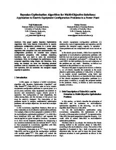
Optimization, Genetic Algorithm, Test case, Generation,. Design, Testing. 1. INTRODUCTION. Computer software assessment is one of the majorities of.
Jun 13, 2012 - transferability by comparison to DFT calculations of strained bulk structures, quantum wells with varying thickness ..... Note that a large supercell with ideal bulk atomic positions leads ..... Email: [email protected]. 1 E. Fermi .
tials are generated from single-valence-electron configurations and satisfy a norm-conservation ... valence electrons (silicon) and a transition metal atom (titanium) are given. .... correctly the following quantities in the reference configura-.
THE SCENARIO GENERATION ALGORITHM FOR MULTISTAGE ...... The restriction operator rk restricts a function u with domain Î to the current scenario tree T ...
Nov 4, 2015 - Keywords Black-Box Noisy Optimization · Algorithm Selection ..... evaluations per iteration, dedicated to running the M solvers (one evaluation.
28-31 www. pim-journal.org○C World Academic Publishing. 28 .... The formulation is given by Agapiou [8]:. 60 π. = ∙. ≤. ∙. ∙ ∙ ∙ ∙ c r e cs m useful. D e. P. P. a z F N.
STEP (2) : Compare Pareto Individuals with the one in the. Long-term and .... The KUR problem has closed relation of the neighbors' variables in ( ) xf. 1.
The Newton Raphson algorithm is an iterative procedure that can be used to ...
The first part of developing the Newton Raphson algorithm is to devise a way to ...
Algorithm visualization, code interpretation, pseudocode, automatic animation ..... pseudocode converted to Python programming language. Python code is ...
Algorithm visualization, code interpretation, pseudocode, automatic animation ..... pseudocode converted to Python programming language. Python code is read-only, but .... informatike-Pseudo-kod-katalog.pdf (accessed on. 15.02.2013).
... a Japanese word that means âcompass bearingâ, the puzzle is a simple 8x8 square grid containing ... various Shinro video games [1][2][3] and web sites [4][5].
We predict that 112H is the most stable hydride in the Group 12 series due to relativistic effects. .... pseudopotentials for the group 11 and group 12 elements,28.
Constructing pseudopotentials for ABINIT: about the use of the fhi98PP package.
Martin Fuchs. Fritz-Haber-Institut der Max-Planck-Gesellschaft, Berlin, Germany.
Aug 1, 2016 - Structural Mechanics and Analysis of Constructions., 1 (2015), pp. ... [22]; I.N. Serpik, A.V. Alekseytsev, RU Certificate of official registration of ...
Dec 11, 2009 - Abstract. The paper presents an application of Levenberg-Marquardt algorithm to parametric optimization of the minimax type of measurement ...
optimization results of all algorithms are tabulated (Table. Table 2. Retaining structure assembly unit price. (Yepes et al., 2008). Item. Unit. Unit price (USD/m).Missing:
and the intercept method implementing an account of nonlinear behavior of the bearing ... where acrc is the opening width of transverse cracks in concrete, acrc,ult .... [2] X.-S. Yang, A new metaheuristic bat-inspired algorithm, in Nature Inspired .
curacy of the chosen electronic structure method. ... to reference data for highly charged single-valence-electron .... mth group of the periodic table, we chose.
Feb 4, 2015 - arXiv:1502.01200v1 [cond-mat.mtrl-sci] 4 Feb 2015. Correlated Electron Pseudopotentials for 3d-Transition Metals. J. R. Trailâ and R. J. Needs.
Fort Collins-Loveland Water District. Fort Collins, Colorado. Optimization techniques applied to water distribution networks have been the topic of much research ...
Optimization Algorithm for the Generation of ONCV Pseudopotentials
Feb 3, 2015 - III, we introduce the quality function to assess the performance ..... iI. BeS BeT e. BP BS b. C. O. C. G e. C. P b. N a. C l. N a. I. M g. S. M g. T e. A.
Optimization Algorithm for the Generation of ONCV Pseudopotentials Martin Schlipf∗ and Fran¸cois Gygi† Department of Computer Science, University of California Davis, Davis, CA 95616, USA
arXiv:1502.00995v1 [cond-mat.mtrl-sci] 3 Feb 2015
We present an optimization algorithm to construct pseudopotentials and use it to generate a set of Optimized Norm-Conserving Vanderbilt (ONCV) pseudopotentials for elements up to Z=83 (Bi) (excluding Lanthanides). We introduce a quality function that assesses the agreement of a pseudopotential calculation with all-electron FLAPW results, and the necessary plane-wave energy cutoff. This quality function allows us to use a Nelder-Mead optimization algorithm on a training set of materials to optimize the input parameters of the pseudopotential construction for most of the periodic table. We control the accuracy of the resulting pseudopotentials on a test set of materials independent of the training set. We find that the automatically constructed pseudopotentials provide a good agreement with the all-electron results obtained using the FLEUR code with a plane-wave energy cutoff of approximately 60 Ry.
I.
INTRODUCTION
Pseudopotentials were introduced over three decades ago as an elegant simplification of electronic structure computations.1 They allow one to avoid the calculation of electronic states associated with core electrons, and focus instead on valence electrons that most often dominate phenomena of interest, in particular chemical bonding. In the context of Density Functional Theory (DFT), pseudopotentials have made it possible to solve the Kohn-Sham equations2,3 using a plane-wave basis set, which considerably reduces the complexity of calculations, and allows for the use of efficient Fast Fourier Transform (FFT) algorithms. The introduction of normconserving pseudopotentials (NCPP) by Hamann et al. in 19794,5 greatly improved the accuracy of DFT plane wave calculations by imposing a constraint (norm conservation) in the construction of the potentials, thus improving the transferability of potentials to different chemical environments. More elaborate representations of pseudopotentials were later proposed, most notably ultrasoft pseudopotentials6 (USPP) and the projector augmented wave7 (PAW) method, improving computational efficiency by reducing the required plane wave energy cutoff. The implementation of these PP is however rather complex,8 in particular for advanced calculations involving hybrid density functionals,9 many-body perturbation theory,10 or density-functional perturbation theory.11 Both USPP and PAW potentials have been used with great success in a large number of computational studies published over the past two decades. NCPP potentials were also widely used but suffered from the need to use a large plane wave basis set for some elements, especially transition metals. Recently, Hamann suggested8 a method to construct optimized norm-conserving Vanderbilt (ONCV) potentials following the USPP construction algorithm without forfeiting the norm-conservation. The resulting potentials have an accuracy comparable to the USPP at a moderately increased plane-wave energy cutoff. Since the very first pseudopotentials were introduced, there has been an interest in a database of transferable,
reference potentials that could be applied for many elements in the periodic table.5,12,13 The need for a systematic database in high-throughput calculations led to a recent revival of this field: Garrity et al.14 proposed a new set of USPP for the whole periodic table except the noble gases and the rare earths. Dal Corso15 constructed a high- and a low-accuracy PAW set for all elements up to Pu. Common to these approaches is the fact that the input parameters of the PP construction are selected by experience based on the results of the allelectron (AE) calculation of the bare atom. The quality of the constructed PP is then tested by an evaluation of different crystal structures and by comparing to the allelectron FLAPW16–18 results. To standardize the testing procedure, Lejaeghere et al.19 suggested to compare the area between a Murnaghan fit20 obtained with the PP and the AE calculation resulting in a quality factor ∆. K¨ u¸cu ¨kbenli et al.21 proposed a crystalline monoatomic solid test, where the quality factor of the simple cubic (sc), body-centered cubic (bcc), and face-centered cubic (fcc) structure is evaluated to assess the quality of a PP. There are two improvements over these construction principles that we propose to address in this work. First, we introduce a quality function that takes into account the computational efficiency of the PP as well as its accuracy. Second, we allow for a systematic feedback of this quality function onto the input parameters defining the PP. In this way, we can introduce an automatic construction algorithm that optimizes the properties of the PP without bias from the constructor. We apply this algorithm to construct ONCV pseudopotentials and compare their performance with recent USPP14 and PAW15 PP libraries. The pseudopotentials are available in UPF and XML format on our webpage.22 This paper is organized as follows: In Sec. II, we outline the properties of the ONCV PP and introduce the input parameters that will be optimized by the algorithm. In Sec. III, we introduce the quality function to assess the performance of the PP, specify the materials we use to construct and test the PP, outline the setting of the DFT calculation, and finally present the optimization algorithm that iterates construction and testing until a good PP is found. We compare the constructed PP to results
2 obtained with FLAPW, USPP, and PAW in Sec. IV and draw our conclusions in Sec. V II.
energy by evaluating the eigenvalues en and eigenvectors ξnR ϕi = ϕ0 +
ONCV PSEUDOPOTENTIALS
NX −M
xn ξnR .
(4)
n=1
The optimized norm-conserving Vanderbilt (ONCV) pseudopotentials were recently proposed by Hamann.8 Here, we briefly sketch their construction, following Hamann, to highlight the input parameters (bold in text) that determine the properties of the PP. The general idea is introduce an upper limit wave vector qc and optimize the pseudo wave functions ϕi (r) such that the residual kinetic energy Z ∞ dq q 4 ϕi (q)ϕj (q) (1) Eij (qc ) = qc
above this cutoff is minimized. Here, ϕi (q) is the Fourier transform of the pseudo wave function Z ∞ ϕi (q) = 4π dr r2 jl (qr)ϕi (r) , (2) 0
jl (qr) a spherical Bessel function, and l the angular moment of the pseudo wave function. On the one hand, the cutoff qc determines which features of the physical potential can be described by the PP. On the other hand, increasing qc makes the PP harder and hence more costly to evaluate. For every angular moment, a projector radius rc determines in which region the pseudoization is done. The projector radius is approximately inversely proportional to the cutoff qc so that a smaller value increases the computational cost along with the accuracy. Outside of this radius the wave function should follow the true all-electron wave function ψ. To ensure the continuity at this radius, one imposes M constrains on the continuity of the pseudo wave function dn ϕ dn ψ = , drn rc drn rc
(3)
for n = 0, . . . M − 1. In this work, we use M = 5 for all constructed PP. The basis set used in the optimization is constructed from spherical Bessel functions. As the basis functions are only used inside the sphere, they are set to zero outside of the projector radius. This destroys the orthogonality of the basis, so that one needs to orthogonalize it again. A linear combination of the orthogonalized basis functions yields a new basis where a single basis function ϕ0 satisfies the constraints in Eq. (3) and for all other basis functions ξnN the value and the M − 1 derivatives at rc are zero. As a consequence, the sum of ϕ0 and any linear combination of the ξnN will satisfy the constraints in Eq. (3). It is advantageous to select those linear combinations of ξnN that have a maximal impact on the residual
In this work, we construct the PP with N = 8 basis functions. Notice that the optimization of the pseudo wave function is performed under the constraint that the norm of the all-electron wave function is conserved. From the obtained pseudo wave functions, one can construct projectors χi χi (r) = (εi − T − Vloc )φi (r) ,
(5)
where T is the kinetic energy operator. Vloc is the local potential that follows the all-electron potential outside of rc and is extended smoothly to the origin by a polynomial. For occupied states εi is the eigenvalue of the all-electron calculation. For unoccupied states, one needs to specify this energy shift before the construction of the PP. Following Ref. 8, we construct two projectors per angular momentum l ≤ lmax and only the local potential for all l > lmax above. The projectors define the following nonlocal potential X
χi B −1 χj VNL = (6) ij ij
where
Bij = ϕi χj ,
(7)
which is a Hermitian matrix when normconserving pseudo wave functions are constructed.6 One can simplify this potential by a unitary transformation to the eigenspace of the B matrix. III.
COMPUTATIONAL DETAILS A.
Quality function
In order to employ numerical optimization algorithms in the construction of PPs, we need a function that maps the multidimensional input parameter space onto a single number, the quality of the PP. A good PP is characterized by a small relative deviation AE δaPP = aPP lat /alat − 1 lat
(8)
between the lattice constant obtained in the planeAE wave PP calculation aPP lat and in the AE calculation alat , respectively. A second criterion is the plane-wave energy cutoff Ecut necessary to converge the PP calculation. These two criteria compete with each other because the pseudoization of the potential reduces the necessary energy cutoff at the cost of a lower accuracy near the nucleus. Hence, we need to specify a target accuracy δ0
3 40 Ry 60 Ry 90 Ry 140 Ry
quality function
30
20
10
0
0
0.1
0.2 0.3 δ in %
0.4
0.5
FIG. 1: (Color online) Quality function for various energycutoffs Ecut . For small δ, it is proportional to 1/Ecut ; for large δ proportional to 1/δ 2 and independent of Ecut .
which we want to achieve for our PP, i.e., for all mate ≤ δ0 . We select δ0 = 0.2% motivated by the rials δaPP lat fact that the choice of different codes or input parameters in the all-electron calculation may already lead to a relative error of approximately 0.1%. To discriminate between PPs within the target accuracy, we include a term ∝ 1/Ecut in the quality function, favoring smoother PP over PP hard ones. For PPs that are significantly outside δa > 2δ0 our target accuracy, we only focus on optilat mizing the relative deviation by an 1/(δaPP )2 term. We lat choose a smooth continuation between the two regions, resulting in the function depicted in Fig. 1. The quality function has the following form ( A + Cδ 2 + Dδ 3 + Eδ 4 + F δ 5 δ < 2δ0 q(δ, Ecut ) = 2 (2δ0 /δ) δ ≥ 2δ0 (9) with 1280 Ecut 32y0 − 16A − 29 C= 4δ03 96y0 − 33A − 122 E= 16δ04 A=1+
The function can be multiplied by an arbitrary scaling constant, which we set such that the value of the quality = 2δ0 . function is 1 at δaPP lat B.
Sets of materials
As the constructed pseudopotentials depend on the set of materials used in the optimization algorithm, it is im-
portant that the set contain physically relevant environments of the atom. Furthermore, we select highly symmetric structures with at most two atoms per unit cell to reduce the computation time. As representatives of a metallic environment, we select the simple cubic (sc), the body-centered cubic (bcc), the face-centered cubic (fcc), and the diamond-cubic (dc) structure. Ionic environments are provided in a rock-salt or zinc-blende structure, where we combine elements such that they assume their most common oxidation state. This leads to a combination of elements from the lithium group with the fluorine group, the beryllium group with the oxygen group, and so on. We always use the three smallest elements of the respective groups to guarantee a variation in size of the resulting compounds. For the transition metals, several oxidation states are often possible. Hence, we combine them with carbon, nitrogen, and oxygen to test these different valencies. As the noble gases do not form compounds, we test them only in the sc, bcc, fcc, and dc structure. Finally, we need to separate these materials into two sets. The training set consists of the bcc, and the fcc structure as well as all rock-salt compounds. It is used in the optimization algorithm to construct the PPs. As the PPs are specifically optimized to reproduce the structural properties of the training set, we can only judge if the PPs are highly accurate by calculating an independent test set. The test set contains the sc and the dc structure as well as all zinc-blende compounds. In total, the training and test sets consist of 602 materials, where every noble-gas atom is part of four materials, and every other element is part of at least ten materials.
C.
Computational setup
All pseudopotentials are constructed using the PerdewBurke-Ernzerhof (PBE) generalized gradient density functional.23 We use an 8 × 8 × 8 Monkhorst-Pack kpoint mesh in the AE as well as in the PP calculation. While this may not be sufficient to completely converge the lattice constant with respect to the numbers of kpoints, the errors in the PP and the AE calculation are expected to be the same, so that we can still compare the results. To ensure that metallic systems converge, we use a Fermi-type smearing with a temperature of 315.8 K corresponding to an energy of 0.001 htr. For the AE calculation, we use the FLAPW method as implemented in the Fleur code.24 We converge the plane-wave cutoff and add unoccupied local orbitals to provide sufficient variational freedom inside the muffintin spheres. The precise numerical values necessary to converge the calculation are different for every material; all input files can be obtained from our web page.22 We obtain the lattice constant by a Murnaghan fit20 through 11 data points surrounding the minimum of the total energy. The automatic construction of pseudopotentials re-
4
0.6
δ (%)
0.4
0.2
0
−0.2 40
60
80
100 120 Ecut (Ry)
140
160
FIG. 2: (Color online) Relative deviation δ of a PP w.r.t. the AE calculation. The blue circles indicate the deviation obtained at a certain energy cutoff Ecut . The red diamonds show the corrected deviation that is monotonically decreasing with increasing cutoff (see text).
quires every material to be calculated several hundred times. Hence, we approximate the Murnaghan equation of state by a parabola that we fit through data points at the AE lattice constant and a 1% enlarged or reduced value. We test the constructed PP with the Quantum ESPRESSO25 plane-wave DFT code. Our test consists of a calculation with a large energy cutmax off of Ecut = 160 Ry that we consider to be the converged solution. Then, we decrease the cutoff in steps of ∆E = 10 Ry to the minimum of 40 Ry. Notice that as illustrated by Fig. 2, the actual deviation compared to the AE calculation may decrease even though we reduced the accuracy of the calculation. To correct for this, we adjust the deviation such that it is monotonically decreasing using the following correction
PP i max δcorr (Ecut ) = |δ PP (Ecut )| +
i X
k−1 k |δ PP (Ecut ) − δ PP (Ecut )|
of materials with the geometric average of all involved materials. In the case of the rock-salt compounds, we test always only one of the PP and for the other element we use a PP from the GBRV database.14 After (N + 1) PP have been constructed, we employ a NelderMead algorithm26 to optimize the PP further. The PP parameters form a simplex in an N dimensional space. By replacing the worst corner by a better PP the simplex contracts towards the optimal PP. The advantages of the Nelder-Mead algorithm are that we do not need to know the derivatives with respect to the input parameters and that it can find PP parameters that lie outside of the starting simplex. After 80 to 200 iterations of the Nelder-Mead algorithm, all PP have converged. Then, we restart the algorithm using these first generation PP as starting guess. Now, we employ the first generation PP in the compounds so that our resulting PP become independent of the GBRV database. Once the second generation is converged as well (another 100 iterations), the properties of the training set are well reproduced for almost all materials.
E.
Refining the training set
For a few materials, the second generation PP do not reproduce the AE results on the test set of materials. Our proposed optimization algorithm provides an easy solution to overcome these cases by adding additional materials to the training set. In particular, for the early transition metals (Sc to Mn) it is necessary to include the sc structure in the training set. Furthermore, we include the dimer of hydrogen and nitrogen into the test set, because the second generation PPs for these two elements do not describe the bond length of the dimer accurately. We emphasize that our optimization algorithm could account for other material properties. As long as one is able to define a quality function, which maps the result of a PP potential calculation onto a number, it is possible to optimize the input parameters of the PP generation by standard numerical optimization techniques.
k=1
(10) i max where Ecut = Ecut − 10i. This ensures that the deviation at a given cutoff energy is an upper bound to the deviation at any larger cutoff. D.
Optimizing pseudopotentials
We start from a reasonable starting guess for the N input parameters. We used the example input files provided with the ONCVPSP package,8 where available, or generated our own PP otherwise. By randomly altering all input parameters in the starting-guess PP by a small amount, we can construct new PP. We assess these PP by evaluating the quality function on the training set
IV.
RESULTS
We compare the performance of the ONCV PP constructed in this work (SG15)22 with the USPP in the GBRV database14 and the high-accuracy PAW in the PSLIB.15 For the latter, we generate the potentials of PSLIB version 1.0.0 with Quantum ESPRESSO version 5.1.1. In the first subsection, we focus on the lattice constants and bulk moduli of the materials in the training set. In the second subsection, we investigate the materials in the test set. In the third subsection, we look into materials that are not represented in the test set to check the accuracy of the pseudopotentials. In the first
5 TABLE I: Comparison of the performance of the USPP in the GBRV database14 and the high-accuracy PAW in PSLIB15 with the ONCV PP in the SG15 database (this work) for materials in a bcc structure. We analyze the relative deviation of the lattice constant δalat and the bulk modulus δB0 between a PP and the AE calculation. The average reveals if the PP has a systematic bias and the root-mean-square (rms) average tests the size of the error. We also show the proportion of materials that are not accurately described at various energy cutoffs. average δalat (%) rms average δalat (%) % of materials with |δalat | > 0.2%a % of materials with |δalat | > 0.2%b % of materials with |δalat | > 0.2%c average δB0 (%) rms average δB0 (%) % of materials with |δB0 | > 5.0%a % of materials with |δB0 | > 5.0%b % of materials with |δB0 | > 5.0%c total number of materials a With b With c With
an energy cutoff of 40Ry. an energy cutoff of 60Ry. an energy cutoff of 160Ry.
two subsections, we focus only on the trends across all materials in the training and test set, respectively.
A.
Training set
In Table I, we present the results obtained for the materials in a bcc structure. We see that the USPP potentials require the smallest energy cutoff and have the best performance at 40 Ry. On the other hand increasing the energy cutoff beyond 40 Ry hardly improves the results. For the PAW and the ONCV PP, a large number of materials are not converged at 40 Ry, but increasing the energy cutoff improves the accuracy, so that they are able to improve on the USPP results. For the converged calculation, the root-mean-square (rms) error is around 0.1% for all PP and smallest for the ONCV PP. We see a similar trend for the bulk moduli though the converged results require a larger energy cutoff on average. The average error for the converged bulk moduli is roughly 3% and the USPP potentials converge with a lower energy cutoff than the PAW and the ONCV PP, which have a similar convergence behavior. In Fig. 3, we see that only for two materials (carbon and calcium) does the converged lattice constant deviate by more than 0.2% with the ONCV PP. For both of these materials the USPP and the PAW approach show large deviations as well. The fcc structures presented in Table II follow the same trend as the bcc structures. The USPP potentials require
TABLE II: Same as Table I for fcc structures. average δalat (%) rms average δalat (%) % of materials with |δalat | > 0.2%a % of materials with |δalat | > 0.2%b % of materials with |δalat | > 0.2%c average δB0 (%) rms average δB0 (%) % of materials with |δB0 | > 5.0%a % of materials with |δB0 | > 5.0%b % of materials with |δB0 | > 5.0%c total number of materials a With b With c With
an energy cutoff of 40Ry. an energy cutoff of 60Ry. an energy cutoff of 160Ry.
TABLE III: Same as Table I for rocksalt structures. average δalat (%) rms average δalat (%) % of materials with |δalat | > 0.2%a % of materials with |δalat | > 0.2%b % of materials with |δalat | > 0.2%c average δB0 (%) rms average δB0 (%) % of materials with |δB0 | > 5.0%a % of materials with |δB0 | > 5.0%b % of materials with |δB0 | > 5.0%c total number of materials a With b With c With
an energy cutoff of 40Ry. an energy cutoff of 60Ry. an energy cutoff of 160Ry.
the smallest energy cutoff but can not be improved further by increasing the energy cutoff. The PAW and the ONCV PP require a energy cutoff of 60 Ry to converge most materials, but have fewer inaccurate elements when increasing the energy cutoff. Overall the ONCV PP and the PAW are a bit better than the USPP, but all PP are close to the AE results. In Fig. 3, we see that only a single material (cadmium) is outside the 0.2% boundary, when using the converged calculation and the ONCV PP. The USPP result shows a deviation of similar size for this material, whereas the PAW lattice constant is close to the FLAPW result. When combining two materials to form rock-salt compounds, we obtain the results depicted in Table III. In comparison to the metallic (bcc and fcc) system, the accuracy for the ionic compounds is a bit higher in particular for the bulk modulus. With a large energy cutoff the ONCV PPs essentially reproduce the AE results and the
He Be C O Ne Mg Si S Ar Ca Ti Cr Fe Ni Zn Ge Se Kr Sr Zr Mo Ru Pd Cd Sn Te Xe Ba Hf W Os Pt Hg Pb
He Be C O Ne Mg Si S Ar Ca Ti Cr Fe Ni Zn Ge Se Kr Sr Zr Mo Ru Pd Cd Sn Te Xe Ba Hf W Os Pt Hg Pb
6
0.3
0.3
0.2
0.2
0.1
0.1
0
0
-0.1
-0.1
-0.2
-0.2
-0.3
-0.3
-0.4
-0.4
HCl HI LiCl LiI BeS BeTe BP BSb CO CGe CPb NaCl NaI MgS MgTe AlP AlSb SiO SiSn KF KBr CaO CaSe ScN ScAs TiN VC VO CrN MnC MnO FeN CoC CoO NiN CuC CuO ZnS GaN GaAs GaBi RbF RbBr SrS YN YAs ZrN NbC NbO MoN TcC TcO RuN RhC RhO PdN AgC AgO CdS InN InAs CsF CsBr BaS LaN LaAs HfN TaC TaO WN ReC ReO OsN IrC IrO PtN AuC AuO HgS TlN TlAs
H Li B N F Na Al P Cl K Sc V Mn Co Cu Ga As Br Rb Y Nb Tc Rh Ag In Sb I Cs La Ta Re Ir Au Tl Bi
0.4
H Li B N F Na Al P Cl K Sc V Mn Co Cu Ga As Br Rb Y Nb Tc Rh Ag In Sb I Cs La Ta Re Ir Au Tl Bi
0.4
0.4 0.3 0.2 0.1 0 -0.1 -0.2 -0.3
HF HBr LiF LiBr BeO BeSe BN BAs BBi CSi CSn NaF NaBr MgO MgSe AlN AlAs AlBi SiGe SiPb KCl KI CaS CaTe ScP TiC TiO VN CrC CrO MnN FeC FeO CoN NiC NiO CuN ZnO ZnSe GaP GaSb GeO RbCl SrO SrSe YP ZrC ZrO NbN MoC MoO TcN RuC RuO RhN PdC PdO AgN CdO CdSe InP SnO CsCl BaO BaSe LaP HfC HfO TaN WC WO ReN OsC OsO IrN PtC PtO AuN HgO HgSe TlP PbO
-0.4
FIG. 3: (Color online) Relative change δ(%) of the lattice constant in the training set for the SG15 (red circle), the GBRV (green square), and the PSLIB (blue diamond) results as compared to the FLAPW ones for the bcc (top left), fcc (top right) and rock-salt compounds (bottom).
accuracy at 60 Ry for the lattice constant is very good. For the bulk modulus, about 10% of the materials require a larger energy cutoff. The USPPs have a slightly larger mismatch for the lattice constants, but converge both lattice constants and bulk moduli with 40 Ry. The PAW potentials provide a similar convergence behavior as the ONCV potentials; they deviate a bit more for the lattice constants, but provide slightly better bulk moduli. In Fig. 4, we show a histogram of the relative error of the lattice constant for all the examined PP (with the converged cutoff of 160 Ry). The histogram confirms the conclusions we drew from Table I to III: All PPs show a very good agreement with the all-electron results and the USPPs have a slightly lower accuracy. The tails with large errors are very flat indicating that there are only a few outliers.
B.
Test set
In the sc structure (see Table IV), the performance of the ONCV potentials is comparable to the training set for the lattice constants and slightly worse for the bulk moduli. We observe the same trend also for the USPP and the PAW calculations. With an overall deviation of about 0.1% for the lattice constant and 4% for the bulk moduli, all PPs show a good agreement with the AE reference data. The convergence with respect to the energy cutoff is best in the GBRV database, which does not change significantly for the lattice constants above 40 Ry. Most of the ONCV lattice constants converge at 60 Ry whereas PAW occasionally needs a larger cutoff. For the bulk moduli, all PPs show a similar convergence behavior. However, we observe that as compared to the other
FIG. 4: (Color online) Histogram of the relative error of the lattice constant compared to the all-electron result. We show the results for all materials in the training set for the SG15 (red solid line), the GBRV (green dotted line), and the PSLIB (blue dashed line) calculations.
TABLE IV: Same as Table I for sc structures. average δalat (%) rms average δalat (%) % of materials with |δalat | > 0.2%a % of materials with |δalat | > 0.2%b % of materials with |δalat | > 0.2%c average δB0 (%) rms average δB0 (%) % of materials with |δB0 | > 5.0%a % of materials with |δB0 | > 5.0%b % of materials with |δB0 | > 5.0%c total number of materials a With b With c With
an energy cutoff of 40Ry. an energy cutoff of 60Ry. an energy cutoff of 160Ry.
structures a larger fraction of > 10% is not accurate even with an energy cutoff of 160 Ry. In Fig. 5, we see that the ONCV PPs reproduce the lattice constant within the 0.2% boundary for all materials except calcium and lanthanum. While the ONCV PP gives similar results to the other PP for calcium, we find that the lattice constant in lanthanum is underestimated by the ONCV PP and overestimated by the USPP. For this material, the PAW calculation did not converge. In Table V, we present our results for the materials in the diamond structure. These are the structures which exhibit overall the largest deviation from the all-electron result. The lattice constants of the USPPs are converged well with the energy cutoff of 40 Ry, whereas the PAW
average δalat (%) rms average δalat (%) % of materials with |δalat | > 0.2%a % of materials with |δalat | > 0.2%b % of materials with |δalat | > 0.2%c average δB0 (%) rms average δB0 (%) % of materials with |δB0 | > 5.0%a % of materials with |δB0 | > 5.0%b % of materials with |δB0 | > 5.0%c total number of materials a With b With c With
an energy cutoff of 40Ry. an energy cutoff of 60Ry. an energy cutoff of 160Ry.
TABLE VI: Same as Table I for zincblende structures. average δalat (%) rms average δalat (%) % of materials with |δalat | > 0.2%a % of materials with |δalat | > 0.2%b % of materials with |δalat | > 0.2%c average δB0 (%) rms average δB0 (%) % of materials with |δB0 | > 5.0%a % of materials with |δB0 | > 5.0%b % of materials with |δB0 | > 5.0%c total number of materials a With b With c With
an energy cutoff of 40Ry. an energy cutoff of 60Ry. an energy cutoff of 160Ry.
and the ONCV PP frequently require a cutoff of 60 Ry. For the bulk moduli, we find that the ONCV PP provide the best agreement with the AE results. The quality of the USPP is similar, but the PAW potentials show an average error larger than the desired 5% tolerance. However the fraction of materials that are well described with the PP calculation is similar for all methods. This indicates that a few specific materials show a particular large deviation, whereas the rest is accurately described. For the ONCV PPs the lattice constants of boron, chlorine, scandium, nickel, rubidium, and yttrium deviate by more than 0.2% from the FLAPW results. In Fig. 5, we observe that the deviations between the different pseudoizations are larger than for the other structures. A possible explanation is that the diamond structure is a extreme case for many materials, because of its low space filling. For the zincblende compounds (cf. Table VI), we ob-
He Be C O Ne Mg Si S Ar Ca Ti Cr Fe Ni Zn Ge Se Kr Sr Zr Mo Ru Pd Cd Sn Te Xe Ba Hf W Os Pt Hg Pb
He Be C O Ne Mg Si S Ar Ca Ti Cr Fe Ni Zn Ge Se Kr Sr Zr Mo Ru Pd Cd Sn Te Xe Ba Hf W Os Pt Hg Pb
8
0.3
0.3
0.2
0.2
0.1
0.1
0
0
-0.1
-0.1
-0.2
-0.2
-0.3
-0.3
-0.4
-0.4
HCl HI LiCl LiI BeS BeTe BP BSb CO CGe CPb NaCl NaI MgS MgTe AlP AlSb SiO SiSn KF KBr CaO CaSe ScN ScAs TiN VC VO CrN MnC MnO FeN CoC CoO NiN CuC CuO ZnS GaN GaAs GaBi RbF RbBr SrS YN YAs ZrN NbC NbO MoN TcC TcO RuN RhC RhO PdN AgC AgO CdS InN InAs CsF CsBr BaS LaN LaAs HfN TaC TaO WN ReC ReO OsN IrC IrO PtN AuC AuO HgS TlN TlAs
H Li B N F Na Al P Cl K Sc V Mn Co Cu Ga As Br Rb Y Nb Tc Rh Ag In Sb I Cs La Ta Re Ir Au Tl Bi
0.4
H Li B N F Na Al P Cl K Sc V Mn Co Cu Ga As Br Rb Y Nb Tc Rh Ag In Sb I Cs La Ta Re Ir Au Tl Bi
0.4
0.4 0.3 0.2 0.1 0 -0.1 -0.2 -0.3
HF HBr LiF LiBr BeO BeSe BN BAs BBi CSi CSn NaF NaBr MgO MgSe AlN AlAs AlBi SiGe SiPb KCl KI CaS CaTe ScP TiC TiO VN CrC CrO MnN FeC FeO CoN NiC NiO CuN ZnO ZnSe GaP GaSb GeO RbCl SrO SrSe YP ZrC ZrO NbN MoC MoO TcN RuC RuO RhN PdC PdO AgN CdO CdSe InP SnO CsCl BaO BaSe LaP HfC HfO TaN WC WO ReN OsC OsO IrN PtC PtO AuN HgO HgSe TlP PbO
-0.4
FIG. 5: (Color online) Relative change δ(%) of the lattice constant in the test set for the SG15 (red circle), the GBRV (green square), and the PSLIB (blue diamond) results as compared to the FLAPW ones for the sc (top left), diamond (top right) and zincblende compounds (bottom).
serve results similar to for the rock-salt compounds. We find that the USPPs converge for most materials with an energy cutoff of 40 Ry, whereas a third of the materials with ONCV PP and half of the materials with PAW need an energy cutoff of 60 Ry to converge. Overall the accuracy of the ONCV PP is slightly better than the alternatives, but all pseudoizations are on average well below the target of 0.2%. For the bulk moduli a larger energy cutoff is necessary, but when converged the deviation from the AE results is around 1%. In Fig. 5, we identify that only for BeO the deviation between the ONCV calculation and the AE result is larger than 0.2%.
shows a slightly larger deviation than the PAW and the ONCV PP. The histogram reveals that this is partly due to some outliers, for which the lattice constant is overestimated by more than 0.4%. Overall, we notice that the accuracy of the ONCV PP for the test set of materials is not significantly worse than for the training set. Hence, we are confident that these PP are transferable to other materials as well.
In Fig. 6, the histogram of the relative error of the lattice constant for the test set confirms the conclusions we drew from Table IV to VI: The deviation from the all electron results is very small for all PP. The USPP
Our training and test set are limited to mono- and diatomic crystals, hence one may wonder if the constructed ONCV PPs work outside this scope. To test this we investigated diatomic molecules and ternary compounds.
FIG. 6: (Color online) Histogram of the relative error of the lattice constant compared to the all-electron result. We show the results for all materials in the test set for the SG15 (red solid line), the GBRV (green dotted line), and the PSLIB (blue dashed line) calculations.
TABLE VII: Bond length of diatomic molecules and lattice constant of perovskites and half-Heusler compounds investigated with different methods. For the half-Heusler compounds, the first element is in Wyckoff position c. All values are given in ˚ A. material H2 N2 O2 F2 Cl2 Br2 AsNCa3 BaTiO3 KMgCl3 LaAlO3 PNCa3 SrTiO3 BScBe GeAlCu NiScSb NMgLi PdZrSn PZnNa
a We evaluate the lattice constant perovskites and half Heusler with FLAPW and take the bond length of the dimers from the CCCB DataBase.27
For the compounds, we use the same computational setup as for the materials in the training and in the test set. For the molecules, we optimize the bond length inside a box with dimensions 15 ˚ A × 15 ˚ A × 30 ˚ A with the long side parallel to the axis of the molecule. In Table VII, we show the bond lengths and the lattice constants of the investigated materials. Depending on the pseudoization, some diatomic molecules show large deviations from the reference data from the CCCB DataBase.27 Overall, the ONCV PPs exhibit the smallest deviations. The relative error is larger than 0.2% only for the O2 (0.25%) and the F2 (0.35%) dimer. For the USPP, all diatomic molecules are outside of the desired relative accuracy of 0.2%, except for the Br2 dimer. In PAW, the only molecule with the desired accuracy is the H2 dimer. The other molecules show deviations of similar magnitude to the USPP and the Br2 dimer did not converge. Perovskites are accurately described by all pseudoizations; we frequently find a relative agreement of better than 0.1% in the lattice constant with the FLAPW result. The worst case for the ONCV PP is LaAlO3 , which deviates by −0.13%. The USPP and the PAW both overestimate the lattice constant of BaTiO3 by 0.25% and 0.27%, respectively. The PAW potentials also feature a larger deviation than the other two pseudoizations for SrTiO3 . Finally, we consider the half-Heusler compounds. All materials are within the desired accuracy with all pseudoizations. The ONCV PP show slightly larger deviations than USPP and PAW for GeAlCu and NMgLi. For NiScSb, the ONCV PP and PAW overestimate the lattice constant more than the USPP. The lattice constant of BScSb and PdZrSn are essentially the same with FLAPW and in any pseudoization used. In PZNa, all PP produce very similar results and a slightly larger lattice constant than the FLAPW result.
V.
CONCLUSION
We have presented an algorithm to optimize the input parameters of a pseudopotential (PP) construction. We demonstrated it by developing the SG15 dataset22 of ONCV pseudopotentials, which exhibits a similar accuracy as the ultrasoft PP database GBRV14 and the PAW library PSLIB.15 The idea of the algorithm is to map the PP onto a single numeric value so that standard optimization techniques can be employed. For this, we developed a quality function that considers the accuracy of the lattice constant of a PP calculation and compares it with a high accuracy FLAPW one. In addition, the quality function takes into account the energy cutoff necessary to converge the calculation. Hence, the optimzation of the PP with respect to the quality function yields accurate and efficient potentials. In order to ensure that the constructed PPs are of a high accuracy, we systematically chose a set of approximately 600 materials and
10 TABLE VIII: Summary of the results depicted in Table I to VI with same notation as Table I. average δalat (%) rms average δalat (%) % of materials with |δalat | > 0.2%a % of materials with |δalat | > 0.2%b % of materials with |δalat | > 0.2%c average δB0 (%) rms average δB0 (%) % of materials with |δB0 | > 5.0%a % of materials with |δB0 | > 5.0%b % of materials with |δB0 | > 5.0%c total number of materials a With b With c With
an energy cutoff of 40Ry. an energy cutoff of 60Ry. an energy cutoff of 160Ry.
evaluate their properties with FLAPW. We split this set in two parts, a training set used for the optimization of the PP and a test set to analyze the performance of the PP. When a PP does not produce our desired accuracy after optimizing on the training set, we can improve the quality of the PP by extending the training set by more materials. In Table VIII, we collect the results of all materials in test and training set. Compared to the PP from the GBRV database14 and PSLIB,15 the PP in the SG15 set have the lowest root-mean-square deviation from the FLAPW results for the lattice constant. With an energy cutoff of 60 Ry, the ONCV PP feature the least number of materials with an inaccurate lattice constant (deviation larger than 0.2% from FLAPW results). The advantage
∗ † 1 2 3 4 5
6 7 8 9
10 11
Electronic address: [email protected] Electronic address: [email protected] See e.g. R. M. Martin, Electronic Structure. Basic Theory and Practical Methods, Cambridge University Press, 2004. P. Hohenberg and W. Kohn, Phys. Rev. 136, B864 (1964). W. Kohn and L. J. Sham, Phys. Rev. 140, A1133 (1965). D. R. Hamann, M. Schl¨ uter, and C. Chiang, Phys. Rev. Lett. 43, 1494 (1979). G. B. Bachelet, D. R. Hamann, and M. Schl¨ uter, Phys. Rev. B 26, 4199 (1982). D. Vanderbilt, Phys. Rev. B 41, 7892 (1990). P. E. Bl¨ ochl, Phys. Rev. B 50, 17953 (1994). D. R. Hamann, Phys. Rev. B 88, 085117 (2013). A. D. Becke, J. Chem. Phys. 98, 1372 (1993); ibid. 98, 5648 (1993). F. Aryasetiawan and O. Gunnarsson, Rep. Prog. Phys. 61, 237 (1998). S. Baroni, P. Giannozzi, and A. Testa, Phys. Rev. Lett. 58, 1861 (1987).
of the ultrasoft PP is that they offer a similar accuracy with an energy cutoff of 40 Ry. For the bulk moduli larger energy cutoffs are necessary for all pseudoization methods. The ONCV PP have the smallest root-meansquare deviation for the tested materials. The fraction of materials that can be accurately described with the ONCV PP at a certain energy cutoff is very similar to the performance of the PAW. The ultrasoft PP exhibit a similar accuracy at a moderately lower energy cutoff. For materials that go beyond the training and test set, we find that the ONCV PP provides the best description of diatomic molecules. All pseudopotentials are very accurate for perovskite and half-Heusler compounds. We encourage the community to use the algorithm presented in this work to optimize pseudopotentials for different functionals and with different construction methods. With only a modest increase in the energy cutoff, the proposed SG15 library of norm-conserving pseudopotentials provides a competitive alternative to the libraries using USPP and PAW. As these pseudopotentials are less complex than the alternatives, this results in a great simplification in the development and implementation of new algorithms.
Acknowledgments
This work was supported by the US Department of Energy through grant DOE-BES de-sc0008938. An award of computer time was provided by the DOE Innovative and Novel Computational Impact on Theory and Experiment (INCITE) program. This research used resources of the Argonne Leadership Computing Facility at Argonne National Laboratory, which is supported by the Office of Science of the U.S. Department of Energy under contract DE-AC02-06CH11357.
12
13 14
15 16
17
18 19
20 21
N. Troullier and J. L. Martins, Phys. Rev. B 43, 1993 (1991). C. Hartwigsen, S. Goedecker, and J. Hutter, Phys. Rev. B 58, 3641 (1998). K. F. Garrity, J. W. Bennett, K. M. Rabe, and D. Vanderbilt, Comp. Mater. Sci. 81, 446 (2014). A. Dal Corso, Comp. Mater. Sci. 95, 337 (2014). E. Wimmer, H. Krakauer, M. Weinert, and A. J. Freeman, Phys. Rev. B 24, 864 (1981). M. Weinert, E. Wimmer, and A. J. Freeman, Phys. Rev. B 26, 4571 (1982). H. J. F. Jansen and A. J. Freeman, Phys. Rev. B 30, 561 (1984). K. Lejaeghere, V. Van Speybroeck, G. Van Oost, and S. Cottenier, Crit. Rev. Solid State Mater. Sci. 39, 1 (2014). F. Murnaghan, Proc. Nat. Acad. Sci. USA 30, 244 (1944). E. Kucukbenli, M. Monni, B. Adetunji, X. Ge, G. Adebayo, N. Marzari, S. de Gironcoli, and A. D. Corso, arXiv:1404.3015 .
11 22 23
24 25
http://www.quantum-simulation.org J. P. Perdew, K. Burke, and M. Ernzerhof, Phys. Rev. Lett. 77, 3865 (1996). http://www.flapw.de. P. Giannozzi, S. Baroni, N. Bonini, M. Calandra, R. Car, C. Cavazzoni, D. Ceresoli, G. L. Chiarotti, M. Cococcioni, I. Dabo, A. Dal Corso, S. de Gironcoli, S. Fabris, G. Fratesi, R. Gebauer, U. Gerstmann, C. Gougoussis, A. Kokalj, M. Lazzeri, L. Martin-Samos, N. Marzari, F. Mauri, R. Mazzarello, S. Paolini, A. Pasquarello, L.
26
27
Paulatto, C. Sbraccia, S. Scandolo, G. Sclauzero, A. P. Seitsonen, A. Smogunov, P. Umari, and R. M. Wentzcovitch, J. Phys.: Condens. Matter 21, 395502 (19pp) (2009). J. A. Nelder and R. Mead, The Computer Journal 7, 308 (1965). NIST Computational Chemistry Comparison and Benchmark Database, NIST Standard Reference Database Number 101, Release 16a, edited by R. D. Johnson III (August 2013).