Generic Switching Actions of Distribution System Operation Using

Generic Switching Actions of Distribution System Operation Using Dynamic Programming Method Yenn-Ming Tzeng1

1

Department of Electrical Engineering Fortune Institute of Technology Kaohsiung, Taiwan.

2

Yu-Lung Ke2*

Meei-Song Kang3

Member, IEEE

Member, IEEE

Department of Electrical Engineering Kun Shan University Tainan, Taiwan. *corresponding author

Abstract-The distribution system configuration can be modified using line switches. This approach enables the loading of line segments and distribution feeders to be adjusted to obtain the load balance and enhance the system performance due to loss minimization resulting from the presented generic switching actions. This paper develops the optimal switching actions for the 22.8KV underground distribution system within the Taichung distribution automation system (DAS) in the Taiwan Power Company (Taipower) system. The dynamic programming method (DP) is designed to determine the optimal switching actions for a single day via feeder reconfiguration. Keywords: distribution system, dynamic programming (DP), switching action, load balance, feeder reconfiguration.

I. INTRODUCTION The problems of protection coordination, line voltage drop and feeder losses result from overloaded or unbalanced three-phase [1] distribution feeder caused by uneven load demand of distribution feeders comprising the various combinations of customer types within service zones. This paper is more practical and conducted the state derivation of line switches during feeder reconfiguration [2, 3] based on the customer load survey [4, 5] combining the derived models [6] of load variation to calculate the load demand of every service section in the distribution feeders. The 22.8KV underground distribution automation system involving three substations, six main transformers, 18 distribution feeders and 79 four-way line switches in the Taichung district

of the network of Taipower is studied in this paper. First, the hourly load data for the distribution feeder are collected and the hourly load demand in every service zone is determined according to analysis of load composition in the various service zones. The problems of load balance or loss reduction [7-9] are identified using the dynamic programming method to examine the hourly distribution system configuration with minimal loss or feeder configuration with optimal load balance. Figure 1 shows the flowchart for the proposed solution methodology.

1-4244-0336-7/06/$20.00 ©2006 IEEE.

1

3

Department of Electrical Engineering Kao Yuan University Kaohsiung, Taiwan.

II. DYNAMIC PROGRAMMING APPLICATION TO OPTIMAL SWITCHING ACTIONS

optimized switching operations of distribution system during a single day. First, the 24 hours of the day are divided into 24 stages, each of which is divided into several states based on the probable combinations of switching operations. The corresponding state cost in each state is determined based on the cost function defined by the initially desirable optimal system state. Finally, the optimal system execution strategy is developed based on the backward recursive DP method. The backward recursive DP algorithm approach is expressed by Eq. (1).

Dynamic programming (DP), a mathematical programming methodology, is suitable for interrelation decision making in time series. The switching operations of a distribution system under constraints are set to provide a programmable optimal flowchart for solving an optimized scheme or strategy via the proposed dynamic programming method. Dynamic Programming Theorem Dynamic programming divides a single problem into several stages with a decision having to be made during each stage. Dynamic programming can provide several system states for selection during each stage. The decision made during each stage determines the transition from the current state to some state in the next stage according to decision conditions such as certain criteria, probability distributions or other settings. The global optimal execution scheme for the overall problem is formed by the proposed approach integrating the optimal selection during each stage. The optimal practical strategy in every state during the overall solution process is determined via the backward procedure started at the final stage. When the recursive relationship reverse search method is adopted to determine the solution for the study system, the reverse backward procedure is executed stage by stage. The optimal strategy during that stage is determined during each backward procedure until the optimal strategy during the first stage is identified. The optimal strategy during every state at stage n can be found and the optimal strategy during every state at the (n+1) stage can be determined using the recursive relationships.

F ∗ (t, ξ t ) = Min {C state (t , ξ t ) + C trans ⋅ ϖ (t + 1, t ) ξ t +1

(1)

∗

+ F ( t + 1, ξ t +1 )}

where: Cstate (t), Ctrans (t): the state and operation costs at stage t, respectively. ξ t : states of all feeder switches at stage t. ϖ(t + 1, t) : operation switching times from stage t+1 to stage t.

F * (t , ξ t ) : the minimal accumulated objective function

up to stage t.

{t + 1, ξ t +1} : the set of all practical states at stage t+1. The above backward recursive DP method during the execution process must satisfy the following constraints of Eqs. (2) and (3). 24

∑ SWi (t) ⊕ SWi (t − 1) ≤ K i

(2)

t =1 where

ˆI ≤ I i rated

(3) SWi (t) = 1: the status of switch i at stage t is closed. SWi (t) = 0: the status of switch i at stage t is open. Ki: the permitted maximal switching operation times for switch i. Irated: the rated current of the distribution feeder or main transformer. ⊕ =exclusive OR operation

Solution Approach for Dynamic Programming This study utilizes the backward recursive relationship to represent the dynamic programming model for optimizing the optimal combination of line switches. The derivation steps for expressing the DP model for optimizing the combination via backward recursive DP are as follows. Step 1. The study problem is assembled by several stages and defines the corresponding states at each stage. Step 2. Build the states at any stage and select the system evaluation standard required to conduct the decision-making during various stages. Step 3. Determine the relationships between the states during various stages and those in the next stage during the establishment of the model structure. Step 4. The decision-making process during the stage only relates to the related system states and system evaluation criteria. Step 5. Complete the independent decision-making at various stages using the above derivation step by step, namely the optimal path in pace with time variation is then determined.

 SWi (t) ⊕ SWi (t −1) =1 when SWi (t) ≠ SWi (t −1)    SWi (t) ⊕SWi (t − 1) = 0 when SWi (t) = SWi (t − 1)

(4)

The current Iˆi in Eq. (3) obtained via power flow analysis must be less than that of the rated current of distribution feeders during switching operations to avoid main transformer overloading. The data in the pick-up feeders and release feeders are updated following a switching operation. Each state involved in a stage t is defined using the likely switching operation combinations based on the network configuration during the previous stage t-1, enabling the realization of the time series relationships using the DP approach. Figure 2 illustrates the state diagram for backward recursive DP and searching paths. Stage 0 represents the initial stage. Dynamic programming is designed to find all possible paths and the ultimate goal is to find a path that satisfies both the constraints conditions by Eqs. (2) and (3)

Application of Dynamic Programming Method to Optimal Switching Actions This paper applies the DP approach to complete hourly 2

and minimizes the value calculated in Eq. (1). Switching operation strategies are designed mainly to consider only load balance among distribution feeders, release the overloading or consider system losses. This study combines several objective functions and constraints into a multi-objective state cost to simultaneously handle the load balance and system losses.

to determine probable combinations of switching operations and the corresponding load balance cost Cbalance and the system state cost Cstate. The load distribution among distribution feeders is mostly balanced using the proposed switching operation pairs and corresponding state cost Cstate via the optimized network configuration obtained using the dynamic programming approach. The operation cost Ctrans includes the artificial and line switch operation costs, where the line switch cost for each switching operation is defined as the total cost in each line switch divided by the total switching operation times in each line switch. The total line switch operation cost is then calculated as the product of the line switch cost in each switching operation and the switching operation times from the previous stage to present stage.

III. COST FUNCTION FOR LOAD BALANCE Cost function for load balance is mainly designed to achieve an optimized network structure for balancing loads among distribution feeders and main transformers to provide sufficient load transfer margin and enhance operating efficiency. Balancing the loads among distribution feeders and main transformers requires first finding all normal-open tie switches in the distribution system. The optimal load balance switching operation pairs are derived to enable the appropriate transfer of the partial loadings of heavy-loaded feeders to light-loaded feeders, not only relieving the overloading problem of heavy-loaded feeders, but also reducing system losses. The load balance index between the heavy and light loaded feeders is calculated using Eq. (5). ∆ C b = ((

I i, old I ave

)2 + (

I j, old I ave

) 2 ) − ((

I i, new I ave

)2 + (

I j, new I ave

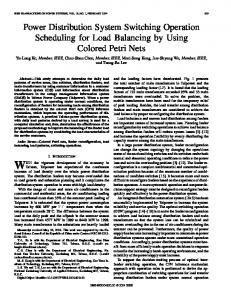
IV. COMPUTER SIMULATIONS The partially underground distribution system of the Taichung distribution automation system comprises three substations, six main transformers, 90 service sections and 79 line four-way switches, and is selected for computer simulations to demonstrate the effectiveness of optimal switching operation using the proposed dynamic programming method. The daily load profiles of distribution feeders in various substations differ markedly owing to the various served customers served in Fig. 3, where substation #1 mainly provides electricity for industrial users, substation #2 provides electricity for residential customers and substation #3 provides electricity for commercial users. Figure 4 displays the daily real power curve of feeder HJ52 in substation #1. Meanwhile, Figs. 5 and 6 show the daily real power patterns of feeder HJ61 and HJ74 in substations #2 and #3, respectively.

) 2 ) (5)

where △ Cb:load balance index function Ii,old:current in a heavy-loaded feeder before switching. Ij,old:current in a light-loaded feeder before switching. Ii,new:heavy-loaded feeder current following load transfer switching. Ij,new:light-loaded feeder current following load transfer switching. Iave:average current between heavy-loaded and light-loaded feeders.

DAILY MINIMAL LOSS CONFIGURATION To demonstrate the effectiveness of the developed optimal switching operations for maintaining hourly minimal loss using dynamic programming methodology, a study distribution system containing 18 feeders is adopted for computer simulations. Table I lists the execution results for the minimal loss network configuration, where the initial loss represents the hourly loss without any switching operation and the minimum loss indicates the hourly loss following optimal switching operations. During the periods from 1AM to 7AM and from 11AM to 21PM, the distribution network lacks any switching operation because of the load curve during the study periods being smooth. All switching operations are concentrated from 7AM to 10AM and from 21PM to 23PM, due to these two loads rapidly increasing and declining. Figure 7 illustrates the loss comparison before and following switching operations. The total energy saving was 146.2kWh in a single day and over 10kWh per hour from 11AM to 5PM, demonstrating a very clear effect.

△ Cb ＞0 indicates the positive cost reduction effect after switching, and shows that the loadings among distribution feeders are nearly balanced. Otherwise, if △ Cb ＜ 0 represents the cost after switching operations are increased and the effect of cost reduction is negative, the loading distribution among distribution feeders becomes more imbalanced. Load balance of distribution system can be improved by the daily optimal network configuration derived by the dynamic programming approach via the proposed switching operation pairs. The load balance cost function of distribution system is determined via Eq. (6). N

C

balance

= K

∑

b

• ( i =1

I ave − I i I ave

)

(6)

where Cbalance: load balance cost function Kb: load balance cost Iave; average current of N feeders Ii: current in the ith feeder The corresponding load balance cost function Cbalance can be determined using Eq. (6) after completing the load balance switching. Consequently, the hourly loading profile of the study distribution system can be considered one stage 3

Initial State

~ X1, N

~ X 2, M

Cstate, N1

Cstate, M1

Cstate, N2

Cstate, M 2

Cstate, N3

Cstate, M3

K Cstate , P1

...

Cstate, MM

Stage 1

Stage 2

...

Cstate, NN

K Cstate ,P 2

K Cstate , P3

...

... Stage 0

~ X K, P

...

K Cstate , PP

Stage K

Fig..2. State diagram and searching paths in the backward recursive dynamic programming approach.

Fig. 3. One-line diagram of the study distribution system 4

10

Table II shows the hourly load balance cost and cost reduction under the initial and minimal loss network configurations. The timing of the study distribution system in performing the minimal loss switching operations can also improve the problem of load balance among distribution feeders. The loss reduction increases with increasing cost reduction, consistent with the theoretic derivation. Figure 8 shows the cost reduction curve of the study distribution system over a 24 hour period.

MW

8 6 4 2 0

Table I. Hourly loss reduction for the study distribution system switching minimal loss reduction time initial loss operation loss (kWH) (hr) (kWH) times and pairs (kWH) 1 93.5 91.9 1.6 0 2 82.7 81.2 1.5 0 3 75.1 73.5 1.6 0 4 68.9 67.3 1.6 0 5 63.7 61.8 1.9 0 6 62.1 60.1 1.9 0 7 67.9 65.9 2.0 0 1 8 110.0 107.0 3.0 (53,48) 1 9 169.7 163.5 6.2 (69,34) 1 10 193.9 185.5 8.5 (72,35) 11 243.1 231.2 11.9 0 12 245.9 233.7 12.2 0 13 251.2 239.1 12.1 0 14 257.3 245.0 12.3 0 15 255.7 243.4 12.2 0 16 256.5 244.3 12.2 0 17 258.6 247.2 11.4 0 18 252.5 243.5 9.0 0 19 259.9 252.9 7.0 0 20 248.5 242.6 5.9 0 21 219.4 214.5 4.9 0 1 22 159.0 157.3 1.6 (35,72) 2 23 131.6 129.7 1.9 (34,69)(48,53) 24 100.3 98.6 1.7 0 Total 4126.9 3980.7 146.2 6

1 2 3 4 5 6 7 8 9 10 11 12 13 14 15 16 17 18 19 20 21 22 23 24

HOUR Fig. 4. Daily real power curve of feeder HJ52

10 8 MW

6 4 2 0 1 2 3 4 5 6 7 8 9 10 11 12 13 14 15 16 17 18 19 20 21 22 23 24

HOUR Fig. 5. Daily real power curve of feeder HJ61

12 10

MW

8 6 4 2 0 1 2 3 4 5 6 7 8 9 10 11 12 13 14 15 16 17 18 19 20 21 22 23 24

HOUR Fig. 6. Daily real power curve of feeder HJ74

1.2

initial loss (kWh)

1

loss after switching operations

300

0.8

250

0.6

KW

200 150

0.4

100

0.2

50

0

0

1 2 3 4 5 6 7 8 9 10 11 12 13 14 15 16 17 18 19 20

1 2 3 4 5 6 7 8 9 10 11 12 13 14 15 16 17 18 19 20 21 22 23 24

-0.2

HOUR

HOUR

Fig. 7 Loss reduction comparison before and after the switching operation

Fig. 8. Cost reduction curve of the study distribution system over a 24 hour period

5

DAILY

OPTIMAL

LOAD

Table III. Load balance costs for the optimal load balance configuration of the distribution system load switching load balance load balance time balance operation times cost cost under (hr) cost under minimal loss reduction and switching pair initial loss 1 3.24375 2.66321 0.58054 0 2 3.30013 2.71895 0.58118 0 1 3 3.40523 2.74989 0.65534 (20,21) 4 3.46879 2.75735 0.71144 0 3 [(22SW1,22SW2) 5 3.46665 2.6183 0.84835 (69SW1,69SW2)] (61SW1,61SW2)] 6 3.6197 2.69595 0.92375 0 7 3.75127 2.71988 1.03139 0 1 8 3.50911 2.41454 1.09457 (21,20) 4 (22SW1,22SW2) 9 3.10662 2.10904 0.99758 (48SW1,48SW2) (69SW1,69SW2) (3SW1,3SW2) 10 3.69753 2.32189 1.37564 0 1 11 3.93195 2.50379 1.42816 (35,3) 2 12 4.33873 2.79084 1.54789 (61SW1,61SW2)] [(68,69)] 13 4.33704 2.75151 1.58553 0 14 4.34078 2.76732 1.57346 0 15 4.40281 2.80361 1.5992 0 16 4.39689 2.77393 1.62296 0 17 4.36968 2.73034 1.63934 0 18 4.26121 2.69803 1.56318 0 1 19 3.85052 2.60075 1.24977 (47SW1,47SW2) 1 20 3.46103 2.42749 1.03354 (48SW1,48SW2) 21 3.24780 2.28539 0.96241 0 1 22 3.10833 2.21608 0.89225 (68SW1,68SW2) 2 23 3.05024 2.33789 0.71235 (3,35)(47SW1,47S W2) 24 3.25402 2.64737 0.60665 0 Total 88.91981 62.10334 26.81647 17

BALANCE

CONFIGURATION This study investigates the hourly optimal switching operation strategies for balancing loads among distribution feeders in a single day using dynamic programming. Table II lists the load balance cost and cost reduction of the study distribution system before and after the execution of optimal load balance switching operations. Table III shows various hourly system losses under the original and optimal load balance configurations. Figure 9 compares two curves. The reduction in load balance cost exceeds the minimal loss cost reduction when only considering load balance using dynamic programming. Moreover, Fig. 10 shows that the load balance loss reduction is less than the loss reduction under the minimal loss configuration.

loss reduction

Table II. Load balance cost for minimizing the loss of the distribution system load load switching balance cost cost reduction time balance cost operation under by load (hr) under initial times and minimal balance loss switching pair loss 1 3.24375 3.27063 -0.02688 0 2 3.30013 3.28822 0.01191 0 3 3.40523 3.34376 0.06147 0 4 3.46879 3.37009 0.0987 0 5 3.46665 3.31032 0.15633 0 6 3.6197 3.28823 0.33147 0 7 3.75127 3.25484 0.49643 0 1 8 3.50911 2.98986 0.51925 (53,48) 1 9 3.10662 2.94666 0.15996 (69,34) 1 10 3.69753 2.99311 0.70442 (72,35) 11 3.93195 3.12132 0.81063 0 12 4.33873 3.30024 1.03849 0 13 4.33704 3.25246 1.08458 0 14 4.34078 3.29353 1.04725 0 15 4.40281 3.32509 1.07772 0 16 4.39689 3.29594 1.10095 0 17 4.36968 3.25728 1.11240 0 18 4.26121 3.25357 1.00764 0 19 3.85052 3.27405 0.57647 0 20 3.46103 3.39355 0.06748 0 21 3.24780 3.39141 -0.14361 0 1 22 3.10833 3.27429 -0.16596 (35,72) 2 23 3.05024 3.19864 -0.14840 (34,69)(48,53) 24 3.25402 3.36654 -0.11252 0 Total 88.91981 78.05363 10.86618 6

1.8 1.6 1.4 1.2 1 0.8 0.6 0.4 0.2 0 -0.2 -0.4

load balance

1 2

minimal loss

3 4 5 6 7 8 9 10 11 12 13 14 15 16 17 18 19 20 21 22 23 24

HOUR

Fig. 9. Cost reduction comparison considering load balance and minimal loss configuration

6

load balance

loss reduction(KWH)

15

Taiwan Power Company, "Load Characteristics Survey and Analysis of the Central and Northern Region of the Taipower System", Research Report, April 1998. [7] D. Shirmohammadi and H. W. Hing, "Reconfiguration of Electric Distribution Networks for Resistive Line Losses Reduction," IEEE Trans. on Power Delivery, Vol. 4, No. 2, pp. 1492- 1498, 1989. [8] D. L. Flaten, "Distribution System Losses Calculated by Percent Loading," IEEE Trans. on Power System, Vol. No. 2, 1988, pp. 1263-1269. [9] N. Vempati, et al., "Simplified Feeder Modeling for Load Flow Calculation," IEEE Trans. on Power System, Vol. PWRS-2, No. 1, 1987, pp. 168-174.

minimal loss

10 5 0 1

3

5

7

9

11

13

15

17

19

21

23

-5

-10 -15 hour

Yenn-Ming Tzeng received the B. Sc. Degree in electrical engineering from National Institute of Technology, Taipei, Taiwan in 1989 and received the Ph.D. in electrical engineering from National Sun Yat-Sen University, Kaoshung, Taiwan. Current he works as associate professor in electrical engineering of Fortune Institute of technology. His research interests are in the area of application of geographic information system, and A.I. method to improve the power quality of the power system.

Fig. 10. Loss reduction comparison considering load balance and minimal loss configuration

V. CONCLUSIONS A practical distribution system in Taichung distribution automation area is chosen in this paper to demonstrate the effectiveness of the developed approach for determining optimal switching operations. The line switch states are clearly indicated and can be combined into the feeder automation function in distribution automation (DA) to perform real-time switching operations and also execute the developed switching operations via remote control to promote distribution system performance. The computer simulations provide an important practical reference for Taipower in executing the distribution automation application. This paper determines the switching operations required for hourly optimal network configuration over a single day based on load balance and minimal loss using the dynamic programming approach and considering the load characteristics of the study distribution feeders. The dynamic programming approach integrating reverse search and recursive procedure can provide an efficient and fast method of deriving switching operations to guarantee that the distribution system fits the optimal configuration.

Yu-Lung Ke (M’98) was born in Kaohsiung City, Taiwan, on July 13, 1963. He received his B.S. degree in control engineering from National Chiao Tung University, Hsin-Chu City, Taiwan, in 1988. He received his M.S. degree in electrical engineering. from National Taiwan University, Taipei City, Taiwan, in 1991. He received his Ph.D. degree in electrical engineering from National Sun Yat-Sen University, Kaohsiung City, Taiwan, in 2001. Since August 1991, he has been at the Department of Electrical Engineering, Kun Shan University of Technology, Yung-Kang City, Tainan Hsien, Taiwan. He is presently a full Associate Professor. His research interests include power systems, distribution automation, energy management, power quality, renewable energy and power electronics. Since 2002, Dr. Ke has served as a reviewer for IEEE Transactions on Power Delivery, IEE Proceedings Generation, Transmission and Distribution, International Journal of Electrical Power & Energy Systems and International Journal of Power and Energy Systems. Dr. Ke is a member of IEEE and a registered professional engineer at Taiwan.

References [1] Whei-Min Lin, Mo-Shin Chen, Neil Van Geem, "Feeder Unbalance Check with AM/FM System," Proceeding of the American Power Conference, 1987. [2] C. S. Chen, J. C. Hwang, M. Y. Cho, Y. W. Chen, "Development of Simplified Loss Models for Distribution System Analysis," IEEE Trans. on Power Delivery, Vol. 9, No. 3, July, 1994, pp. 1545-1551. [3] T. P. Wanger, A. Y. Chikhani, R. Hackam, "Feeder Reconfiguration for loss Reduction: An Application of Distribution Automation," 91 WM 101-6, PWRD. [4] C. S. Chen, J.S. Wu, M.T. Tsay, C.T. Liu, "Application of Load Patterns and Customer Information System for Distribution System Analysis," Proceeding of the First International Conference on Power Distribution, Brazil, Nov. 1990. [5] C. S. Chen, J. C. Hwang, Y. M. Tzeng, "Derivation of Class Load Pattern By Field Test for Temperature Sensitivity Analysis," EPSR, Jan. 1996. [6] National Kaohsiung Institute of Science and Technology and

Meei-Song Kang (M’99) received the M.S., Ph.D. degree in Electrical Engineering from the National Sun Yat-Sen University in 1993 and 2001 respectively. Since August 1993, he has been with Department of Electrical Engineering, Kao Yuan Institute of Technology, Kaohsiung, Taiwan. Currently he is an Associate Professor. His research interest is in the area of load survey and demand subscription service.

7