Ï a b . The graph of a. Gaussian is a characteristic symmetric âbell curveâ shape that quickly falls off towards plus/minus infinity. The parameterb is height of curve.
International Journal of Computer Applications (0975 – 8887) Volume 6– No.8, September 2010
Genetic Algorithm Based Comparison of Different SVM Subhash Chandra Pandey
G.C. Nandi
Department of Computer Science Birla Institute of Technology, Ranchi-Allahabad Campus B-7, Industrial Area, Naini,
Indian Institute of Information Technology Deoghat, Jhalwa Allahabad-211012 India
Allahabad-211010, India
ABSTRACT The SVM has recently been introduced as a new learning technique for solving variety of real world applications based on learning theory. The classical RBF network has similar structure as SVM with Gaussian kernel. Similarly, the FNN also possess an identical structure with SVM. The support vector machine includes polynomial learning machine, radial-basis function network, Gaussian radial-basis function network, and two layer perceptron as special cases. Genetic algorithm has been increasingly applied to various search and optimization problems in the recent past but in spite of its broad applicability, ease of use and global perspective, it has not yet been used in comparison and optimization of different support vector machines. In this paper attempt has been made to compare and optimize the rate of convergence of different SVMs by using the concepts of GAs and important results are worked out.
General Terms
[2]. SVR can perform high accuracy and robust properties for function approximation with noise [3]. Some researches have been done on combining SVM and FNN and it is established that support Vector machines (SVMs) and Feed-forward Neural Networks (FNNs) are two alternative machine learning frameworks for classification and regression problems with different inductive bias and very interesting properties [4][7][8][9]. It is worthwhile to say that both schemes have been developed from very different genesis points of view, they exhibit a number of elements that allow to make a direct solutions. As a matter of fact, they are structurally identical, since both SVMs and FNNs induce a function which is expressed as a linear combination of N
simpler functions:
f ( x) = b + ∑ λk h(wk , x) .
In case of
k =1
SVMs, N is the number of support vectors, h is the kernel N
function, {wk }k =1
are the support vectors and
{λ k }kN=1 are the
Soft computing, Evolutionary computation.
coefficient found by the constrained optimization problem posed. For FNNs (fully connected with one hidden layer of units and output linear units), N is the number of units in the hidden
Keywords
layer, h is the activation function,
Support vector machine, Genetic algorithm, Rate of Convergence, Learning.
1. INTRODUCTION The support vector machine is an elegant and highly principled learning method for the design of a FNN network with a single hidden layer of nonlinear units. Its derivation follows the principle of structural risk minimization that is rooted in VC dimension theory, which makes its derivation even more profound. As the name implies, the design of the machine hinges on the extraction of a subset of the training data that serves as support vectors and therefore represents a stable characteristic of the data. The support vector machine includes the polynomial learning machine, radial basis function network, Gaussian radial basis function network, and two layer perceptron as special cases. Although these methods provide different representations of intrinsic statistical regularities contained in training data, they all stem from a common root in a support vector machine setting. Support vector machine performs structural risk minimization and creates a classifier with minimized VC dimension [1]. As the VC dimension is low, the expected probability of error is low to ensure a good generalization. When SVM is employed to tackle the problems of function approximation and regression estimation, it is referred as the support vector regression (SVR)
weights and
{wk }kN=1 are the hidden layer
{λ k }kN=1 are the output-layer weights [10].
As genetic algorithm is a search and optimization tool, which works differently compared to classical search and optimization method, we have made an analysis for the rate of convergence of different types of support vector machines using the concepts of genetic algorithms. The rest of this paper is organized as follows. Section II describes the brief working of the GA. The constrained optimization is discussed in section III. In section IV, theoretical aspects of SVM have been given. Section V describes experimental analysis of different types of SVMs.. Finally, the conclusions are summarized in section VI.
2. GENETIC ALGORITHM Traditional optimization methods can be classified into two distinct groups: direct and gradient-based methods [11]. In direct search methods, only objective function and constraint values are used to guide the search strategy, whereas gradient-based methods use the first and /or second order derivatives of the objective function and/or constraints to guide the search process. That’s why, the direct search methods are usually slow, requiring many function evaluations for convergence and can also be applied to many problems without a major change of the algorithm. 34
International Journal of Computer Applications (0975 – 8887) Volume 6– No.8, September 2010 On the other hand, gradient-based methods quickly converge to an optimal solution, but are inefficient for non-differentiable or discontinuous problems. In addition, traditional techniques suffer from some common difficulties: • •
The convergence to an optimal solution. Most algorithms tend to get stuck to a suboptimal solution. • An algorithm efficient in solving one optimization problem may not be efficient in solving a different optimization problem. • Algorithms are not efficient in handling problems having discrete variables. • Algorithms can not be efficiently used on a parallel machine. Because of the nonlinearities and complex interactions among problem variables, the search space may have more than one optimal solution. When solving such problems, if traditional methods get attracted to any of locally optimal solutions, there is no escape. Further every traditional optimization algorithm is designed to solve a specific type of problems. Further, traditional method can not exploit the convenience provided by the parallel computing machine and it is fact that many complex engineering optimization problems require parallel computing. That’s why genetic algorithm shows precedence over the traditional optimization method. Genetic algorithms are a computational model inspired by evolution. This algorithm encodes the substantial solutions of a problem in a simple chromosome like structure and then apply reproduction, cross-over and mutation operation in way so as to preserve critical information. An implementation of genetic algorithm begins with a population of (typically random) chromosomes. One then evaluates these structures and allocates reproductive. Genetic algorithm works with a coding of variables instead of the variables themselves. Binary GAs works with a discrete search space, even though the function may be continuous. On the other hand, since function values at various discrete solutions are required, a discrete or discontinuous function may be tackle during GAs. This allows GAs to be applied to a wide variety of problem domains. Other advantage is that GA operators exploit the similarities in string-structures to make an effective search. One of the drawbacks of using a coding is that a suitable coding must be chosen for proper working of a GA. Although it is difficult to know before hand what coding is suitable for a problem, a plethora of experimental studies [12] suggest that a coding which respects the underlying building block processing must be used.
3. CONSTRAINED OPTIMIZATION Optimization is a common practice in engineering design. An optimal design problem having N variables is written as a nonlinear programming (NLP) problem, as follows: Minimize
f (x)
Subject to
g j ( x) ≥ 0
hk ( x) = 0 xi
(l )
k = 1,2,.........., K
≤ xi ≤ x i
(u )
i = 1,2,........ ...., N
It
is
possible to convert the constrained NLP problem to an unconstrained minimization problem by penalizing infeasible solutions. A proper choice of penalty parameters is the key aspect of the working of such a scheme. One thumb rule for selection of parameter is that they must be arranged in such a fashion that all penalty terms are of comparable values with themselves and with the objective function values. The penalty corresponding to a particular constraint is very large compared to that of other constraints; the search algorithm emphasizes solutions that do not violate the former constraint. This way other constraints get neglected and search process gets restricted in a particular way [13]. Actually, in most cases, most methods possess tendency of premature convergence to a suboptimal feasible or infeasible solution. It is also a common practice to normalize the constraints so that only one penalty parameter value can be used and the search and optimization method works much better if an approximate penalty parameter value is used [11, 14]. It is well known fact that GAs work with a population of solutions, instead of a single solution. It means a better penalty approach can be used and it also exploits the ability to have pair-wise comparison in tournament selection operator. Fig.1
shows
a
unconstrained
single-variable
function
f (x) which has a minimum solution in the infeasible region.
Fig.1 Constraint handling scheme. Five circles are solutions in a GA population. The fitness F (x ) of any infeasible or feasible solution is defined as follows:
if g j (x) ≥ 0, ∀j ∈ J , f ( x) F ( x) = J f max + ∑j=1 ( g j (x)) otherwise f max is the maximum function value of all feasible the population. The objective function f ( x ) , the
The parameter
j = 1,2,......... ., J
solutions in
35
International Journal of Computer Applications (0975 – 8887) Volume 6– No.8, September 2010 constraint violation g ( x ) , and the fitness function
F ( x) are shown in the figure. It is important to note that F ( x ) = f ( x ) in the feasible region. When tournament selection operator is applied to such a fitness function F ( x ) , all the require criteria will be satisfied and search algorithm will proceed towards the feasible region. The figure also illustrates how the fitness value of five arbitrary solutions will be calculated. Thus, it is obvious that under this constraint handling scheme the fitness value of infeasible solutions may change from one generation to another, but contrary to this, the fitness value of a feasible solution will always be the same. Moreover, the tournament selection does not depend on the exact fitness function values, rather their relative difference is important; any arbitrary penalty parameter will work the same way. As a matter of fact, any explicit penalty parameter is not needed. It is imperative to mention that such constraint handling scheme is possible without the need of a penalty parameter as GAs use a population of solutions and pair-wise comparison of solution is possible by using the tournament selection. From the above discussion, it is explicitly clear that the rate of convergence will be high, if the numbers of infeasible solutions are less. On the other hand, higher number of infeasible solutions will cause a reduced rate of convergence.
An x j with nonzero α j is called a support vector. Let S be the index set of support vectors, then the optimal decision function becomes
f ( x) = sgn ∑ y iα i ( x, xi ) + b i∈S
Where the coefficient α i can be found by solving the dual problem of (1) l
max imize W (α ) = ∑ α i − i =1
to C ≥ α i ≥ 0, i = 1,...., l ,
subject l
and
1 l ∑ α i α j y i y j ( xi , x j ) 2 i , j =1
∑α
i
(3)
yi = 0
i =1
The n
decision boundary given by (2) is a hyperplane in R . More complex decision surfaces can be generated by employing a nonlinear mapping φ feature space
: Rn → F
F (usually
to map the data into a new
has dimension higher than n ), and
finding the maximal separating hyperplane in
4. SUPPORT VECTOR MACHINE
(2)
F.
It should be
noted that in (3) xi never appears isolated but always in the form
This section presents the basic concepts of the SVMs. For gentle tutorials of SVMs, we refer interested readers to [15] and [16]. More exhaustive treatments can be found in [17] and [18]. Let
of inner product ( x i , x j ) . This implies that there is no need to
{(x1, y1),......,(xl , yl )}⊂R ×{+1,−1}be a training set. The SVM
product in
F for
learning
purposes,
instead
n
approach
attempts
to
find
a
canonical
hyperplane {x ∈ R : ( w, x ) + b = 0, w ∈ R , b ∈ R} that maximally separates two classes of training samples. Here,(.,.) is n
n
R n . The corresponding decision function (or n then given classifier) f : R → {+1,−1} is by f ( x ) = sgn(( w, x ) + b). an inner product in
evaluate the nonlinear mapping φ as long as we know the inner any given x, z ∈ R . So for computational n
of
defining φ
: Rn → F
explicitly,
a
: R × R → R is introduced to directly define an inner product in F . Such a function K is also called the Mercer kernel [1] [17] [18]. Substituting K ( xi , x j ) for ( x i , x j ) in (3) function K
n
n
produces a new optimization problem
Considering that the training set may not be linearly separable, the optimal decision function is found by solving the following quadratic program: l 1 j(w, ξ ) = (w, w) + C∑ ξi 2 i =1 subject to yi ((w, xi ) + b) ≥ 1 − ξi , ξi ≥ 0, i = 1,.., l
min imize
where
ξ = [ξ 1 ,......., ξ l ]T are
(1)
slack variables introduced to
allow for the possibility of misclassification of training samples, C > 0 is some constant. Applying the Karush-Kuhn-Tucker complementarity conditions one can show that a w , which minimizes (1), can be written as
∑
l i =1
y i α i xi
. This is called the dual representation of w . 36
International Journal of Computer Applications (0975 – 8887) Volume 6– No.8, September 2010 Table.1 Number of generation required for different SVM
argument x and xi . On the other hand, a translationally and
# genera Types of SVM
tion
Inner product kernel
for Converg ence
Polynomial
T
( X
+ 1)
X
1 exp − X − Xi 2 2σ
RBF
y =
Gaussian Two Layer
P
2
15
− ( x−a )2
1 2 πσ
2
e
2σ
2
17
y = tanh( β 0 X X i + β1 ) T
Perceptron
l
max imize W (α ) = ∑α i − i =1
l
∑α y
i i
100
1 l ∑αiα j yi y j K ( xi , x j ) 2 i , j =1
Gaussian function is a function of the form
i =1
Solving (4) for α gives a decision function of the form
f ( x) = sgn ∑ y iα i K ( x, xi ) + b i∈S
(5)
whose decision boundary is a hyperplane in F , and translates to nonlinear boundaries in the original space. Several techniques of solving quadratic programming problems arising in SVM algorithms are described in [19],[20], and [21]. Details of calculating b can be found in [22].
5. EXPERIMENTAL RESULTS In order to evaluate the performance of the proposed SVMs, experiments have been conducted on MatLab7 and different results are worked out pertaining to convergence of different support vector machines. The learning curves for these SVMs are shown in Fig.2.
5.1 Radial Basis Function 1 The radial-basis function y = exp − 2σ 2 x − xi i specified centre
xi will
basis function. To simplify matters, the condition σ
function
i
=σ
for
−( x−a )2
(4)
Green’s
Here σ i denotes the width of radial-
5.2 Gaussian Function
=0
considered as a
).
convergence. On the other hand, if σ is taken as a constant, an increase in centre will lead an increase in the rate of convergence.
subject to C ≥ α i ≥ 0, i = 1,...., l , and
vector, i.e. G ( x − x i
all i is often imposed. Even though RBF networks thus designed are of a somewhat restricted kind, they are still universal approximators [23]. Table-III shows the area under the infeasible portion of the learning curve of Fig. (2a). It is explicit from the data recorded in the table that for a constant centre value of the function, area below the infeasible portion of curve will increase as σ increases, which in turn, produces a decrease in the rate of
57
rotationally invariant stabilizer D will bound the Green’s function to depend only on the euclidean norm of the difference
f ( x) = be
2σ 2
for some real constants b > 0, a , σ > 0 . The graph of a Gaussian is a characteristic symmetric “bell curve” shape that quickly falls off towards plus/minus infinity. The parameter b is height of curve Table.2 Standard parameter set used for convergence analysis
Parameter
Value
Population size
Pop_size=20
Stopping criteria
Generation=100
Fitness normalization
Rank
Selection operator
Stochastic uniform
Elitism
Elit=2
Crossover
Pc=0.8 Scattered Scale=1.0
2
can be
Mutation
Shrink=1.0 Gaussian
whose characteristic for a
be precluded only by the form of
stabilizer D . In case, when the form of stabilizer D is translationally invariant, be G ( x −
the
Green’s
xi ) dependent
function i.e.
the
centered difference
at xi
will
between
the
37
International Journal of Computer Applications (0975 – 8887) Volume 6– No.8, September 2010 12
Radial Basis Function
x 10
Gaussian 0.2
18
0.18
16
0.16
14
0.14
12
0.12
y
10
y
8
0.1
6
0.08
4
0.06
2
0.04
0
0.02 0
2
4
6
8
10 x
12
14
16
18
20
0
0
2
4
6
8
10 x
12
14
16
18
20
Fig.2 (a) Learning curve for Radial Basis Function Fig.2 (d) Learning curve for GaussianKernel peak, a is the position of the centre of the peak, and σ controls the width of the “bell”. Gaussian functions have wide applications e.g. in statistics they describe the normal distribution. Similarly, in signal processing they serve to define Gaussian filters. The integral of the Gaussian function is called “error function”. Taking the Fourier transform of a Gaussian function with parameter a , b = 0 and σ yields another Gaussian function with
Two Layer Perceptron 1.001
1
0.999
y
parameters b, σ , a
0.997
0.996
0.995
0
2
4
6
8
10 x
12
14
16
18
20
Fig.2 (b) Learning curve for Two-Layer Perceptron 4
18
14 12
y
10 8 6 4 2
0
and 1 / σ
.
So in particular the
2
4
6
8
10 x
It has been observed from the area under the infeasible portion of the learning curve Fig.2 (d) that for a constant value of a , the rate of convergence will increase as the value of σ increases. On the other hand, if σ is kept constant and a is an increase, the area under the infeasible portion of the learning curve will also be increase and thus, cause a decrease in rate of convergence.
5.3 Two-Layer Perceptron
Polynomial
x 10
16
0
=0
Gaussian functions with a = 0 and σ = 1 are kept fixed by the Fourier transforms. Gaussian functions centered at zero minimize the Fourier uncertain principle. The product of two Gaussian functions is again a Gaussian, and the convolution of two Gaussian functions is again a Gaussian.
0.998
12
14
16
18
20
Fig.2(c) Learning curve for Polynomial Kernel
Two-Layer Perceptron can be applied to solve difficult and diverse problems by training them in a supervised manner with a highly popular algorithm known as the error back propagation algorithm. In a two-layer perceptron , the model of each neuron in the network includes a nonlinear activation function and the nonlinearity is smooth. The network contains layers of hidden neurons that are not part of the input or output of the network. These hidden neurons enable the network to learn complex tasks by extracting progressively more meaningful features from the input patterns. The network exhibits a high degree of connectivity which is determined by the synapses of the network. Further, a change in the connectivity of the network requires a change in the population of synaptic connections or their weights. Due to these characteristics two-layer perceptron are also responsible for the deficiencies in our present state of knowledge on the behavior of the network. Owing to presence of a distributed form of nonlinearity and the high connectivity of the network, the theoretical analysis of a two-layer perceptron is difficult to undertake. Further, the use of hidden layers makes the 38
International Journal of Computer Applications (0975 – 8887) Volume 6– No.8, September 2010 visualization of learning process difficult. The learning process is therefore made more difficult because the search has to be conducted in a much larger space of possible functions, and a choice has to be made between alternative representations of the input patterns [24]. Table.4 shows an increase in the number of infeasible solutions as β 0 & β 1 increase (because area under the Table.3
Area
under
the
learning
y=e S.No.
σ
1
2
2
curve
1 x − xi − 2σ 2
Centre Area
σ
2
6.4117e012
2
4
2
0.0019
3
6
2
4
8
5
10
2
infeasible portion of the curve increases) rate of convergence will decrease. On the other hand, a reduced values of β 0 & β 1 increases the rate of convergence. When two-layer perceptron is experimented on MatLab7 by using “gatool”, its convergence shows an oscillating pattern Fig.3 (d). It is also
containing
infeasible
solutions
y =
Centre
for
RBF
Gaussian
− ( x− a )2
1 2 πσ
and
2
e
2σ
2
Area
σ
a
Area
σ
a
Area
2
6.4117e012
2
2
0.8413
2
2
0.8413
2
3
2.0106e010
3
2
0.7475
2
3
0.9332
0.0840
2
4
4.9345e009
4
2
0.6912
2
4
0.9772
2
0.3193
2
5
9.4835e008
5
2
0.6529
2
5
0.9938
2
0.5942
2
6
1.4283e006
6
2
0.6207
2
6
0.9986
xi
xi
Table.4 Area under the learning curve containing infeasible solutions for Polynomial and Two-Layer Perceptron
y = tanh( β 0 x T x i + β 1 )
(1 + x T x )
p
S.No.
p
Area
β0
β1
Area
1
2
6.4365e+00 5
0.25
2/3
1.4703
2
3
1.8474e+00 8
1
2
1.9773
3
4
5.7623e+01 0
2
3
1.9978
4
5
1.8905e+01 3
3
4
1.9998
5
6
6.4142e+01 5
4
5
2.0000
39
International Journal of Computer Applications (0975 – 8887) Volume 6– No.8, September 2010 Best, Worst, and Mean Scores 1
Best, Worst, and Mean Scores 0.2
0.9 0.18
0.8 0.16
0.7 0.14
0.6 0.12
0.5 0.1
0.4
0.08
0.3
0.06 0.04
0.2
0.02
0.1
0
0 0
20
40
60 generation
80
100
120
0
20
(a) Gaussian
40
60 generation
80
100
120
(c) Radial-Basis Function
Best, Worst, and Mean Scores
Best, Worst, and Mean Scores
1.001
250
1 200
0.999 150
0.998 100
0.997
50
0
0.996
0
10
20
30 generation
40
50
0.995
60
(b) Polynomial
0
10
20
explicit from he fig(3) that the rate of convergence of two-layer perceptron is very much less than RBF and Gaussian networks.
5.4 Polynomial A polynomial mapping is a popular method for non-linear modeling. It is of the two types (a) homogeneous
= ( x, x' ) p and
K ( x, x' ) = (1 + x.x' )
p
(b)Nonhomogeneous
40
50 60 generation
70
80
90
100
(d) Two Layer Perceptron
Fig.3. Convergence of different SVM as shown by gatool
i.e., K ( x, x ' )
30
i.e.,
. The second kernel is usually preferable as it avoids problems with hessian becoming zero. Polynomial support vector machines have shown a competitive performance for the problems of pattern recognition. However,
of MATLab 7
there is a large gap in performance vs. computing resources between the linear and quadratic approaches. Taking into account the fitness of a given learning set, the support vector machine minimizes the so called structural risk in order to reach robust generalization for unseen sample.Table4 shows that the rate of convergence of a polynomial SVM decreases as degree increases.
6. CONCLUSION In this paper, a genetic algorithm based method for comparison of rate of convergence of different SVMs has been proposed. First, it is discussed that the rate of convergence will be high if the numbers of infeasible solutions are less. For this purpose, the 40
International Journal of Computer Applications (0975 – 8887) Volume 6– No.8, September 2010 areas below the learning curve, containing the infeasible solutions have been calculated. It is observed that the rate of convergence is maximum for radial-basis function. Further, it has also been analyzed that rate of convergence decreases as σ increase. An increase in value of
xi will
cause increase in convergence rate.
Similarly, for Gaussian function the rate of convergence will be slightly less than the RBF and its rate of convergence increases as σ increases but decreases with increase in a . The convergence analysis of two-layer perceptron shows oscillating pattern. Its rate of convergence is less than the Gaussian and increased values of β 0 & β 1 cause decrease in rate of convergence. Lastly, in polynomial SVM, the rate of convergence decreases as degree of polynomial increases. The convergence of proposed SVMs is also tested on MATLAB7 using “gatool” with different set of parameters. The results obtained are analogous to theoretical analysis.
7. REFERENCES [1] N. Cristianini and J.Showe-Tayler, An Introduction to support vector machine and other kernel based learning methods, Cambridge University Press,2000. [2] V.Vapnik, S. Golowich, and A.J. Smola,Support vector method for function approximation,regression estimation, and signal processing, in neural information processing systems, Cambridge,MA:MIT press,vol.99,1997. [3] C.C. Chuang, S.F.Su,, J.T. Jeng, and C.C.Hsiao, Robust support vector regression network for function approximation with outlier, IEEE Trans.neural networks,vol.13, Nov.2002,pp. 1322-1330. [4] J.H. Chiang, and P.Y. Hao, Support vector learning mechanism for fuzzy rule-based modeling: a new approach., IEEE Trans.Fuzzysyst.vol.2,Feb-2004,pp.1-12. [5] S.Sohn and C.H. Dagli, Advantages of using fuzzy class memberships in self-organising map and support vector machines, Proc international joint conference on neural networks (IJCNN’01),vol.3, july 2001,pp.1886-1890. [6] Z.Sun and Y.Sun,Fuzzy support vector machine for regression estimation, IEEE international conference on systems, man, and cybernetics (SMC’03),vol.4, oct 2003,pp.3336-3341. [7] C.F. Lin and S.D. Wang, Fuzzy support vector machines, IEEE Trans. Neural networks, vol.13,March 2002,pp.464471. [8] Bishop, C.M.: Neural networks for pattern recognition, Oxford univ. press inc., New York, 1995. [9] Vapnik,V.N,The nature theory,springer-verlag,1995.
of
statistical
learning
[12] T. Back, D.Fogel and Z. Michalewiez, (Eds.), Handbook of evolutionary computation, Institute of physics publishing and oxford university press, New York, 1997. [13] K.Deb, An introduction to genetic algorithm, IIT, Kanpur, India [online]. [14] K. Deb and M.Goel, A robust optimization procedure for mechanical component design based on genetic adaptive search, ASME journal of mechanical design (In press). [15] C.L. Blake and C.J. Merz,UCI repository of machine learning databases. Dept. informs. Comput. Sc., Univ. California, Irvine, Irvine, C.A. [Online}.Available:http://www.ics.uci.edu/~mlearn/ML.Rep ository,1998. [16] K.R. Miller, S. Mika, G. Ratsch, K. Tsuda, and B. Scholkopf, An introduction to kernel based learning algorithms, IEEE Trans. neural networks, vol.12,,Apr. 2001, pp. 181-202. [17] V. Vapnik, The nature of statistical learning theory, New york: Springer-verlog, 1995. [18] V. Vapnik, Statistical learning theory, New York:,Weley, 1998. [19] ] T. Joachims, Making large scale SVM learning practical, Advances in kernel methods support vector learning, B. Scholkopf, C.J.C. Burges, and A.J. Smola, Eds, Cambridge, MA: MIT Press, 1999, pp. 169-184. [20] L. Kaufman, Solving the quadratic programming problem arising in support vector classification, Advances in kernel methods-support vector learning. B.Schdkopf, C.J.C. Burges, and A.J. Smola, Eds. Cambridge, MA:MIT Press,1999,pp.147-167. [21] J.C. Platt, Fast training of support vector machines using sequential minimal optimization, Advances in kernel methods-support vector learning, B. Scholkopf, C.J.C. Burges, and A.J. Smola, Eds. Cambridge, MA: MIT Press, 1999, pp. 185-208. [22] C.C. Chang and C.J. Lin, LBSVM: A library for support vector machines, Taiwan [Online], Available: http://www.csie.ntu.edu.tw/~cjlin/libsvm[[[23] Park and Sandberg, Universal approximation using radial basis function networks, neural computation,vol.3(2), 1991,pp. 246-257. [23] Park and Sandberg, Universal approximation using radial basis function networks, neural computation,vol.3(2), 1991,pp. 246-257. [24] Hinton,G.E., Connectionistic learning procedure, Artificial intelligence,vol.40,1989,pp.185-234.
[10] E. Romero and D. Toppo, Comparing support vector machines and feed-forward neural networks with similar parameters, springer-verlag, 2006, pp.90-98. [11] K.Deb, Optimization for engineering design:algorithms and examples,Delhi:Prentice-Hall, 1995
41