SVM based Stock Market Trend Prediction. System. Binoy B. Nair 1 V.P Mohandas 2 N.R. Sakthivel. Amrita School of Engineering, Amrita Vishwa Vidyapeetham.
Binoy B. Nair et. al. / (IJCSE) International Journal on Computer Science and Engineering Vol. 02, No. 09, 2010, 2981-2988
A Genetic Algorithm Optimized Decision TreeSVM based Stock Market Trend Prediction System Binoy B. Nair 1 V.P Mohandas 2 N.R. Sakthivel Amrita School of Engineering, Amrita Vishwa Vidyapeetham Coimbatore, Tamilnadu, India
Abstract—Prediction of stock market trends has been an area of great interest both to researchers attempting to uncover the information hidden in the stock market data and for those who wish to profit by trading stocks. The extremely nonlinear nature of the stock market data makes it very difficult to design a system that can predict the future direction of the stock market with sufficient accuracy. This work presents a data mining based stock market trend prediction system, which produces highly accurate stock market forecasts. The proposed system is a genetic algorithm optimized decision tree-support vector machine (SVM) hybrid, which can predict one-day-ahead trends in stock markets. The uniqueness of the proposed system lies in the use of the hybrid system which can adapt itself to the changing market conditions and in the fact that while most of the attempts at stock market trend prediction have approached it as a regression problem, present study converts the trend prediction task into a classification problem, thus improving the prediction accuracy significantly. Performance of the proposed hybrid system is validated on the historical time series data from the Bombay stock exchange sensitive index (BSE-Sensex). The system performance is then compared to that of an artificial neural network (ANN) based system and a naïve Bayes based system. It is found that the trend prediction accuracy is highest for the hybrid system and the genetic algorithm optimized decision treeSVM hybrid system outperforms both the artificial neural network and the naïve bayes based trend prediction systems. Keywords- ANN, decision tree; genetic algorithm; prediction; stock; SVM; trend;
I.
INTRODUCTION
Stock market prediction has been an area of intense interest due to the potential of obtaining a very high return on the invested money in a very short time. However, according to the efficient market hypothesis [1], all such attempts at prediction are futile as all the information that could affect the behaviour of stock price or the market index must have been already incorporated into the current market quotation. There have been several studies, for example, [2], which question the efficient market hypothesis by showing that it is, in fact, possible to predict, with some degree of accuracy, the future behaviour of the stock markets. Technical analysis has been used since a very long time for predicting the future behaviour of the stock price, but with limited success [3], [4]. The extremely nonlinear nature of the stock market data makes it
ISSN : 0975-3397
very difficult to design a system that can predict the future direction of the stock market with sufficient accuracy. This work presents a data mining based stock market trend prediction system, which produces highly accurate stock market forecasts. The proposed system is a genetic algorithm (GA) optimized decision tree-support vector machine (SVM) hybrid, which can predict one-day ahead trends in stock markets. The uniqueness of the proposed system lies in the use of the hybrid system which can adapt itself to the changing market conditions and in the fact that while most of the attempts at stock market trend prediction have approached it as a regression problem, present study converts the trend prediction task into a classification problem, thus improving the prediction accuracy significantly. Technical indicators are used in the present study to extract information from the financial time series data (stock market daily open, high, low, close and volume) and hence, they act as the features that are given as input to the hybrid system. The trend of the stock market is predicted using a GA-decision tree-SVM hybrid system. The decision tree implemented using the C4.5 algorithm [5] is used for feature selection and the trend prediction is done using SVM. The GA is used to optimize the parameters of the decision tree and the SVM to ensure best prediction accuracy. Once the trend is predicted for the next day, a very simple trading rule is used to decide if stock must be bought, sold or no trade must be carried out to obtain highest possible profit. The flowchart of the proposed system is presented in Fig.1.The designed system is validated on the time series data from Bombay stock exchange sensitive index (BSESensex). The period under consideration is from January 2, 2007 to October 30, 2010. A stand-alone ANN based and a stand-alone Naive Bayes based trend prediction system is also designed and the results are compared. The rest of the paper is organised as follows: Section II presents the design of the proposed hybrid system in detail. Section III presents the experimental results and the conclusions are drawn in section IV. II.
HYBRID SYSTEM DESIGN
The overall design of the system is presented in Fig. 1. The aim is to predict next day’s stock market trend using the historical data in the present day itself and to take a decision on whether to buy, sell or hold the stock when the market
2981
Binoy B. Nair et. al. / (IJCSE) International Journal on Computer Science and Engineering Vol. 02, No. 09, 2010, 2981-2988 starts trading the next day. After the end of each trading day, the stock market data for the day is used to update the system, hence allowing it to adapt to the market dynamics. The key part of the system is the hybrid GA-decision tree-SVM system which predicts the trend for the next day. The proposed hybrid system is realized in four steps. The first step is the feature extraction which involves computation of technical indices from the historical stock market data. Each technical index is a feature. Hence, the terms feature and technical index can be used interchangeably in the present study. Once the technical indices (features) have been computed, the relevant features (technical indices) are selected using a decision tree. The selected features are then used by the support vector classifier to predict the next day’s trend of the stock market. The final step is the GA based optimization of the decision tree and support vector classifier parameters to ensure best possible prediction accuracy. Update stock market historical data Previous day
Extract technical indicators
Stock market trend prediction from the extracted technical indicators using GA optimized Decision tree-SVM hybrid system
Trading rule for next day based on predicted trend
Trade on BSESensex based on the trading rule
Present day
Yes
Stock trading No session over for the day?
A. The Dataset BSE-SENSEX is selected for validation of the proposed trend prediction system. BSE is the world's largest exchange in terms of the number of listed companies (over 4900). It is in the top ten of global exchanges in terms of the market capitalization of its listed companies (as of December 31, 2009). The companies listed on BSE command a total market capitalization of 1.36 trillion US Dollars as of 31st March, 2010. The BSE-Sensex is India's first and most popular Stock Market benchmark index. The stocks that constitute the BSESensex are drawn from almost all the market sectors and hence the BSE-Sensex is capable of accurately tracking the movements of the market. Hence, BSE-Sensex is taken as the representative of the Indian stock markets. Being such a large and complex system, prediction of trends in the BSE-Sensex is especially challenging. B. Feature Generation The inputs of the proposed system are the historical time series data consisting of the daily open, daily high, daily low, daily closing and the trading volumes of the Sensex. Features are generated from this dataset using technical analysis. Twenty eight commonly used technical indexes are considered initially. Technical Indexes considered for the present study are: positive volume index (PVI), negative volume index(NVI), on-balance volume (OBV), typical volume, pricevolume trend, Accumulation/Distribution oscillator, Chaikin’s Oscillator, chaikin’s volatility, acceleration, highest high, lowest low, relative strength index (RSI), moving average convergence/ divergence (MACD) consisting of two indexes, namely, nine period moving average and MACD line, momentum, stochastic oscillator consisting of two indexes%k and %d, typical price , median price, weighted close, william’s %R, price rate of change, williams accumulation/distribution, Bollinger bands consisting of three indexes- Bollinger upper, Bollinger middle and Bollinger lower,25-day moving average, and 65-day moving average. All the twenty eight technical indexes along with the daily stock market data together form the input to the hybrid trend prediction system. Details on technical indicators used in the present study are widely available and a comprehensive treatment of the same can be found in [3] and [4]. Determination of the trend (up, down and no trend) is done in the following way[6]: The market is formally classified as being in an uptrend (downtrend) for the present day when all the following conditions are satisfied: The closing value must lead (lag) its 25 day moving average. The 25 day moving average must lead (lag) 65 day moving average. The 25 day moving average must have been rising (falling) for at least 5 days. The 65 day moving average must have been rising (falling) for at least 1 day.
Figure 1. Flowchart of the proposed hybrid trend prediction system
ISSN : 0975-3397
2982
Binoy B. Nair et. al. / (IJCSE) International Journal on Computer Science and Engineering Vol. 02, No. 09, 2010, 2981-2988 If the movement of the market cannot be classified as either an uptrend or a downtrend, it is assumed that there is no discernable trend in the market movement. The hybrid system will automatically select the features that are necessary for improving trend prediction accuracy. Since the system is continuously learning, the dependency of the prediction accuracy on particular features will change over time, as is seen from the results in section III. C. GA-Decision Tree-SVM Hybrid Trend Prediction System This is the most important part of the proposed system since the next day’s stock trend is predicted using this hybrid system. 1) Decision tree based feature extraction: The Decision tree C4.5 [7] algorithm is widely used to construct decision trees, and has found varied applications in fields including human talent prediction [8] , stock market prediction [9] and stock trading rule generation[20]. It is used in the present study to select the features required for trend prediction. A decision tree is a flowchart-like tree structure, where each internal node (non-leaf node) denotes a test on an attribute, each branch represents an outcome of the test, and each leaf node (or terminal node) holds a class label. The topmost node in a tree is the root node. Given a tuple, for which the associated class label is unknown, the attribute values of the tuple are tested against the decision tree. A path is traced from the root to a leaf node, which holds the class prediction for that tuple. The construction of decision tree classifiers does not require any domain knowledge or parameter setting, and therefore is appropriate for exploratory knowledge discovery.During tree construction, attribute selection measures are used to select the attribute that best partitions the tuples into distinct classes. The attribute selection measure used in the present study is the Gain ratio. It is defined as: Gain ratio (A) = Gain (A) / SplitInfoA (D) Where:
(1)
A is the attribute under consideration. v
SplitInfoA (D) = -
j=1 (
|Dj| / |D| ) log2( |Dj| / |D| )
Gain (A) = Info (D) - InfoA (D) v
InfoA(D) =
j=1
( |Dj| / |D| ) Info ( Dj )
Info(D) = - mi=1 pi log2 pi
(2) (3) (4) (5)
Here, pi is the probability that an arbitrary tuple in D belongs to class Ci and is estimated by Ci,D/ D. The SplitInfoA (D) represents the potential information generated by splitting the training data set, D, into v partitions,
ISSN : 0975-3397
corresponding to the v outcomes of a test on attribute A. The attribute with the maximum gain ratio is selected as the splitting attribute. The Info (D), also known as the entropy of D, is the average amount of information needed to identify the class label of a tuple in D. InfoA(D) is the expected information required to classify a tuple from D based on the partitioning by A. The smaller the expected information still required, the greater the purity of the partitions. Gain (A), ie. the information gain, is defined as the difference between the original information requirement (i.e., based on just the proportion of classes) and the new requirement (i.e., obtained after partitioning on A). The attribute A with the highest information gain, Gain(A), is chosen as the splitting attribute at node N. It can be seen from the above discussion that only those features that are necessary for the classification purpose are included in the tree and the remaining features are not considered at all. This property of decision tree is used in the present study to select the relevant features. The two parameters of the decision tree that need to be optimized in the present study are the minimum number of observations in an impure node for it to be split further and the minimum number of observations required for a node to be labelled as the leaf node. The larger these two values, the smaller will be the tree and consequently, smaller will be the number of selected features. However, the accuracy falls as these two values are increased and the best possible trade-off between tree size and accuracy needs to be found. In the present study, this is accomplished using GA. 2) SVM based trend prediction: SVMs have been used in [10] and [11] for predicting financial time series, and in [12] and[13] to design stock trading/decision support systems. SVM [14] is a learning system based on statistical learning theory. SVM belongs to the class of supervised learning algorithms in which the learning machine is given a set of features (or inputs) with the associated labels (or output values). Each of these features can be looked upon as a dimension of a hyper-plane. SVMs construct a hyper-plane that separates the hyper-space into two classes (this can be extended to multi-class problems).While doing so, SVM algorithm tries to achieve maximum separation between the classes. Separating the classes with a large margin minimises the expected generalisation error. ‘Minimum generalisation error’, means that when a new set of features (that is data points with unknown class values) arrive for classification, the chance of making an error in the prediction (of the class to which it belongs) based on the learned classifier (hyper-plane) should be minimum. Intuitively, such a classifier is one, which achieves maximum separationmargin between the classes. The above process of maximising separation leads to two hyper-planes parallel to the separating plane, on either side of it. These two can have one or more
2983
Binoy B. Nair et. al. / (IJCSE) International Journal on Computer Science and Engineering Vol. 02, No. 09, 2010, 2981-2988 points on them. The planes are known as ‘bounding planes’ and the distance between them is called ‘margin’. SVM ‘learning’ involves finding a hyper-plane, which maximises the margin and minimises the misclassification error. The points lying beyond the bounding planes are called support vectors. [14] has shown that if the training features are separated without errors by an optimal hyper-plane, the expected error rate on a test sample is bounded by the ratio of the expectation of the support vectors to the number of training vectors. The smaller the size of the support vector set, more general the above result. Further, the generalisation is independent of the dimension of the problem. In case such a hyper-plane is not possible, the next best is to minimise the number of misclassifications whilst maximising the margin with respect to the correctly classified features. In order to classify data into C different classes (hence the name, C-Support Vector Classifier or C-SVC), a one-versusrest approach is followed. Here, the class to which the pattern is hypothesized to belong to has a positive distance, i.e. upon substituting in the decision boundary equation, it gives a positive value. For C classes, there are thus C positive or negative decisions. These C one-versus-rest classifiers are compared for the largest positive distance and the classifier that has the largest positive distance is then chosen to be the final decision. The C-SVC is described mathematically as follows: Given training vectors xi ε Rn, i=1,2,..,n in the two-class case and the corresponding class labels decision yi ε {-1, +1}, the C-SVC solves the following optimization problem: Minimize: WT W + C ∑n i=1ξi
(6)
subject to: yi (WT (xi )+b) ≥ (1- ξi ) (7)
K(xixj) = exp(-γ
xi - xj
2
), γ > 0.
(11)
SVMs are described in great detail in [14]. As can be seen from equation (11), the parameter γ of the kernel function needs to be optimized for best classification accuracy. In the present study,this is accomplished using GA. 3) GA based parameter optimization: GA has been very widely used for solving unconstrained optimization problems [15] and is basically parallel search algorithm which can be used for optimizing nonlinear functions, for example, see [16]. Usually, the function which needs to be optimized, called the objective function, takes the shape of a minimization problem. In the present study, GA is used to minimize the trend prediction error (which is another way of saying-maximizing accuracy) by optimizing three parameters, namely, the minimum number of observations in an impure node of a decision tree for it to be split further, the minimum number of observations needed to label the node of a decision tree as the leaf node and the parameter γ of the radial basis function used in C-SVC. In this study, the population size used is 20, the selection mechanism used is the roulette wheel selection, the crossover is uniform and the mutation is Uniform. The lower and upper bounds of the variables are given as (upper bound, lower bound) and are as follows: minimum number of observations in an impure node of a decision tree for it to be split further = ( 1, no. of observations in dataset) minimum number of observations needed to label the node of a decision tree as the leaf node = ( 1, no. of observations in dataset) and parameter γ of the radial basis function= (0,1) 4) Trading rule:
ξi ≥ 0 , i=1,2,..,n Its dual problem is then: minimizeα 0.5( ∑n i=1 αi αj yi yj K(xixj) - ∑n i=1 αi
(9)
0≤ αi ≤ C, i=1,2,..,n Subject to: ∑n i: yi=+1 αi=0, ∑n i: yi=-1 αi=0
(10)
Here, C is the upper bound on the error, and K(xi, xj) is the Kernel Function that describes the behavior of the support vectors, and is equal to K(xi, xj) = Φ(xi)T Φ(xj). It is this function Φ(xi) that transforms the training data into a higher dimension where the support vectors then enable classification by linear decision boundaries. The kernel function considered for the present study is the radial basis kernel function, which is defined as follows:
ISSN : 0975-3397
The trading rule is quite simple and straightforward and unlike the trend prediction system, does not change over a period of time. The trading rule is: If next day’s predicted trend = Uptrend then Buy else if already bought then Hold. Else if next day’s predicted trend= Downtrend then Sell else if no stock in hand then Hold Else if next day’s predicted trend= No trend then Hold. III.
EXPERIMENTAL RESULTS
The performance of the proposed trend prediction system is validated on the BSE-Sensex data. The period under consideration is from January 2, 2007 to October 30, 2010 resulting in 941 observations.
2984
Binoy B. Nair et. al. / (IJCSE) International Journal on Computer Science and Engineering Vol. 02, No. 09, 2010, 2981-2988 A. Hybrid System: The performance of the hybrid system is evaluated using the confusion matrix. When the entire dataset was considered, the hybrid system produced the results as given in Table I: TABLE I.
HYBRID SYSTEM OPTIMISED PARAMETERS
Description
Parameter value or features
Minimum number of observations for the impure node to be split Minimum number of observations for the node node to be made leaf node
70 20
Γ
0.8 MACD line, Chaikin’s volatility, Positive volume index, William’s A/D line, Momentum, daily close
Selected features
The accuracy of the hybrid system is presented in the form of confusion matrix given in Table II. An overall accuracy of 85.54% was obtained. TABLE II.
HYBRID SYSTEM CONFUSION MATRIX
Actual trend
Predicted trend
Uptrend
No trend
Down trend
Up trend
291
48
0
No trend
37
406
36
Down trend
0
15
108
The performance of the hybrid system is compared to that of a stand-alone ANN based trend prediction system and a naïve Bayes based trend prediction system to validate its superiority. B. ANN based system : Artificial Neural Networks (ANNs) offer an alternative to qualitative methods for economic systems that traditional quantitative tools in econometrics cannot quantify due to the complexity in system dynamics[17]. [18], [19], [20], [21], [22], [23] etc. all show that ANNs can outperform conventional statistical approaches. [24] used a feed-forward back propagation network to predict the stocks trading on the Bombay Stock Exchange (BSE) . [25] used feed-forward ANN models for forecasting the BSE sensitive index (BSESensex) with reasonable accuracy. [26] suggested that a single hidden layer feed-forward ANN offers a useful and flexible alternative to fixed specification linear models. Hence, in the present study too, a single hidden layer feedforward network is considered, for acting as another benchmark with which, the proposed system is compared. In a feed-forward neural network, the neurons are usually arranged in layers. A feed-forward neural net is denoted as NI N1 N2 …… Ni … NL NO where:
ISSN : 0975-3397
NI represent the number of input units; i=1,..,L represent the number of hidden layers; NI represent the number of units from the hidden layer I; NO represent the number of output units. The net input to a processing unit j is given by: netj = i wij xi + j
(12)
where xi’s are the outputs from the previous layer, wij is the weight (connection strength) of the link connecting unit i to unit j, and j is the bias of unit j. The objective of different learning algorithms is the iterative optimization of a measure of the performance of the network which is the mean square error. The error for a pattern p is given by Ep
NO
(d j1
pj
y pj ) 2
(13)
where dpj and ypj are the desired and the actual response of the network corresponding to the pattern ‘p’. The total error is P 1 1 P NO E E p (d pj y pj ) 2 (14) 2 p 1 j1 p 1 2 During the training process a set of pattern examples is used, each example consisting of a pair with the input and corresponding target output. The patterns are presented to the network sequentially, in an iterative manner, the appropriate weight corrections being performed during the process to adapt the network to the desired behaviour. This iterating continues until the connection weight values allow the network to perform the required mapping. Each presentation of the whole pattern set is named an epoch. One of the most popular supervised learning algorithms for feed-forward neural networks is Backpropagation. The back propagation learning generally involves the following four steps: Step 1 (Initialization) : Initialize the weights and thresholds of the network. Step 2: (Activation) : Activate the back-propagation neural network by applying inputs x1(p), x2(p),..,xn(p) and desired outputs d1(p),d2(p),…, d,n (p) Step 3: (Weight training) : Update the weights in the backpropagation network by propagating backward the errors associated with output neurons. Step 4: (Iteration) : Increase iteration p by one, go back to Step 2 and repeat the process until the selected error criterion (usually mean square error) is satisfied. There are many variations of back propagation learning algorithms and all of them can be considered as different methods of solving an optimization problem, in which the network tries to find the global minimum value of a function ( in the present case, the function that has to be minimized is the trend prediction error between the actual and the predicted BSE-Sensex trends) . Gradient descent algorithm (Hagan et al. 1996) is the simplest of the back propagation algorithms, but the network using this algorithm can get stuck in a local
2985
Binoy B. Nair et. al. / (IJCSE) International Journal on Computer Science and Engineering Vol. 02, No. 09, 2010, 2981-2988 minimum and hence may never converge to the global minimum. Gradient descent with momentum (GDM) algorithm [27] is a variation of the back propagation algorithm in which an additional ‘momentum’ term is included. This addition of the momentum term prevents the network from getting stuck in a local minimum, thus improving the performance of the network. In this algorithm the minimization of the error function is carried out using a gradient-descent technique. The necessary corrections to the weights of the network for each moment t are obtained by calculating the partial derivative of the error function in relation to each weight wij. A gradient vector representing the steepest increasing direction in the weight space is thus obtained. The next step is to compute the resulting weight update. In it simplest form, the weight update is a scaled step in the opposite direction of the gradient. Hence, the weight update rule is E p (15) Δ w (t) ε (t) p
ij
w
ij
Where (0,1) is a parameter determining the step size and is called the learning rate. A momentum term incorporates in the present weight update, some influence of the past iteration. The weight update rule becomes E p (16) Δ p w ij (t) ε (t) α Δ p w ij (t 1) w ij where is the momentum term and determines the amount of influence from the previous iteration to the present one. The parameters used for the ANN based trend prediction system are given in Table III and the confusion matrix is given in Table IV. The confusion matrix for the naïve Bayes based trend prediction system is given in Table V. TABLE III. Description
Actual trend
Predicted trend
Uptrend
No trend
Down trend
Up trend
176
148
4
No trend
99
357
13
Down trend
11
98
35
C. Naïve Bayes system Bayesian classifiers are statistical classifiers. They can predict class membership probabilities, such as the probability that a given tuple belongs to a particular class. Naïve Bayesian classifiers [7] assume class conditional independence, that is, the effect of an attribute value on a given class is considered independent of the values of the other attributes. It is made to simplify the computations involved and, in this sense, is considered “naïve.” Let X be a data tuple (referred to as ‘evidence’), described by a set of n attributes such that X = (x1, x2 , x3 , x4 ..., xn ) . Assuming that there are m classes, C1, C2,... , Cm, the classifier will predict that X belongs to the class having the highest posterior probability, conditioned on X. By Bayes’ theorem P(Ci|X) = P(X|Ci) P(Ci) / P(X)
(17)
As P(X) is constant for all classes, only P(XCi)P(Ci) need be maximized. The naive assumption of class conditional independence implies P( X|Ci ) = nk=1 P( xk | Ci )
(18)
In the present study, the attributes are continuous and hence, are assumed to have a Gaussian distribution with a mean μ and standard deviation σ,
Parameter value or features Gradient descent with momentum
Architecture
Single layer feed forward network
No. of input neurons
5
No. of hidden neurons
5
No. of output neurons
3
P (xk Ci ) = g(xk, μCi , σCi )
(19)
g (x,,) = ( (2)0.5 )-1 exp ( (x-)2 / 22 )
(20)
Where
In order to predict the class label of X, P(XCi)P(Ci) is evaluated for each class Ci. The naïve Bayesian classifier predicts that tuple X belongs to the class Ci if and only if
Sigmoidal
Learning rate
0.3
Momentum
0.2
From the confusion matrix, it is seen that the ANN based system produces an accuracy of 60.36%.
ISSN : 0975-3397
ANN SYSTEM CONFUSION MATRIX
ANN PARAMETERS
Algorithm
Activation function
TABLE IV.
P(Ci X) > P(Cj X) for 1≤ j ≤ m, j≠ i
(21)
In the present study, three classes are considered: C1= Up, C2= down and C3= no trend. Each X is the set of all the attributes for one day. The naïve Bayes trend prediction system performs the worst with an accuracy of 45.48%, as can be seen from the confusion matrix given in Table V.
2986
Binoy B. Nair et. al. / (IJCSE) International Journal on Computer Science and Engineering Vol. 02, No. 09, 2010, 2981-2988 TABLE V.
NAÏVE BAYES CONFUSION MATRIX
REFERENCES
Actual trend
Predicted trend
Uptrend
No trend
Down trend
Up trend
211
93
24
No trend
231
166
72
Down trend
51
42
51
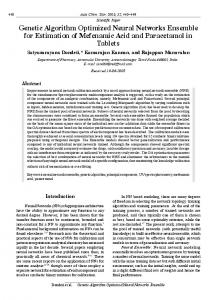
Performance of the systems was also evaluated based on the actual profit generated by the trading system using the predictions made by the three trend prediction systems. For the purpose, all three systems were trained on the stock market data from January 2, 2007 to July30,2010 and the profits generated by the systems from August 2, 2010 to October 29,2010 using the trading rule given in section II was evaluated. It was observed that the hybrid system generated a trading profit of 1083.5 rupees, the ANN based system produced a profit of 729.4 rupees and the Naïve Bayes system produced a loss of 57.6 rupees. The performance of the three systems is summarized in Fig.2.
[1] [2]
[3] [4]
[5] [6] [7] [8]
[9]
[10] [11]
[12]
[13]
[14] [15] Figure 2. Percentage accuracy and profit generated for the systems considered.
IV.
CONCLUSION
This paper presents the design and implementation of a hybrid system for predicting one-day-ahead trends in the stock market. The effectiveness of the proposed system was validated on the BSE-Sensex data. The performance of the proposed system was compared to the performance of an ANN based trend prediction system and a Naïve bayes based system. It was observed that the hybrid system significantly outperforms the other two systems under consideration resulting in more trading profits. Hence, it can be concluded that the proposed hybrid system is well suited for prediction of stock market trends.
[16]
[17] [18]
[19]
[20]
[21]
ISSN : 0975-3397
E. F. Fama , Efficient capital markets: A review of theory and empirical work, Journal of Finance, vol. 25, pp. 383–417,May 1970. G. S.Atsalakis and K. P.Valavanis, “Surveying stock market forecasting techniques – Part II: Soft computing methods”, Expert Systems with Applications, vol. 36 , pp. 5932–5941, 2009. D.R. Jobman, ed.,Technical Analysis for Futures Traders. New Delhi: Vision Books, ,1988. W.F. Eng , The Technical Analysis of Stocks, Options & FuturesAdvanced Trading Systems and Techniques. New Delhi:Vision Books, 1988. J. R. Quinlan, C4.5: Programs for Machine Learning. San Mateo, CA:Morgan Kaufmann, 1993. www. Trend-watch.co.uk. J. Han, and M. Kamber, Data Mining:Concepts and Techniques,2nd Ed., San Mateo, CA:Morgan Kaufmann, 2006. H. Jantan , A.R. Hamdan and Z. A. Othman , “Human talent prediction in HRM using C4.5 classification algorithm”, International Journal on Computer Science and Engineering, vol. 2, no. 8, pp.2526-2534, 2010. M-C.Wu, S-Y. Lin and C-H. Lin, “An effective application of decision tree to stock trading”, Expert Systems with Applications, vol.31, pp. 270–274, 2006. K-J. Kim, “Financial time series forecasting using support vector machines”, Neurocomputing, vol. 55, pp. 307 – 319, 2003. S-H. Hsu, Jj P.-A. Hsieh , T-C. Chih, and K.-C Hsu, “A two-stage architecture for stock price forecasting by integrating self-organizing map and support vector regression”, Expert Systems with Applications, vol.36, pp.7947–7951, 2009. T.V.Gestel, J.A.K. Suykens, D-E. Baestaens, A. Lambrechts, G. Lanckriet, B. Vandaele, B. De Moor and J. Vandewalle, “Financial Time Series Prediction Using Least Squares Support Vector Machines Within the Evidence Framework”, IEEE Transactions on neural networks, vol. 12, no. 4, pp. 809- 821, 2001. W.Huang, Y. Nakamori and S-Y.Wang, “Forecasting stock market movement direction with support vector machine”, Computers & Operations Research, vol.32, no. 10, pp. 2513-2522, 2005. V.N.Vapnik, M. Jordan, S.L. Lauritzen, J.F. Lawless, Nature of Statistical Learning Theory. Berlin: Springer, 1999. D.E Goldberg,Genetic Algorithms in Search, Optimization & Machine Learning. CA:Addison-Wesley, 1989. R.J. Kuo, C.H. Chen and Y.C. Hwang , “An intelligent stock trading decision support system through integration of genetic algorithm based fuzzy neural network and artificial neural network”, Fuzzy Sets and Systems, vol. 118, pp. 21-45, 2001. F.Zahedi, in Intelligent Systems for Business: Expert Systems with Neural Networks, Belmont, USA: Wadsworth , 1993, pp. 10-11. E. W. Saad, D.V. Prokhorov and D.C. Wunsch, “Comparative study of stock trend prediction using time delay, recurrent and probabilistic neural networks”, IEEE Transactions on Neural Networks, vol. 9, no. 6, pp. 1456-1470, November 1998. E.L.de Faria,M.P. Albuquerque, J.L. Gonzalez, J.T.P. Cavalcante and M. P. Albuquerque, “Predicting the Brazilian stock market through neural networks and adaptive, exponential smoothing methods”, Expert Systems with Applications, vol.36, no.10, pp.12506–12509, 2009. E.Vamsidhar, K.V.S.R.P.Varma, P.S. Rao, R. Satapati, “Prediction of rainfall using backpropagation neural network model”, International Journal on Computer Science and Engineering, vol. 2, no. 4, pp. 11191121, 2010. A. Refenes and A. Saidi, “Managing Exchange-Rate Prediction Strategies with Neural Networks”, in Neural Networks in the Capital Market , A. Refenes, Ed. England : John Wiley & Sons , 1995, pp.213219.
2987
Binoy B. Nair et. al. / (IJCSE) International Journal on Computer Science and Engineering Vol. 02, No. 09, 2010, 2981-2988 [22] Y.S.Abu Mostafa, “Financial Market Applications of Learning Hints”, in Neural Networks in the Capital Market , A. Refenes, Ed. England : John Wiley & Sons , 1995, pp. 220-232. [23] M.Steiner and H. Wittkemper, “Neural Networks as an Alternative Stock Market Model” in Neural Networks in the Capital Market , A. Refenes, Ed. England : John Wiley & Sons , 1995, pp.213-219, pp. 137-148. [24] K.S Ravichandran, P. Thirunavukarasu, R. Nallaswamy, R. Babu, “Estimation of Return On Investment In Share Market Through ANN”, Journal of Theoretical and Applied Information Technology, pp. 44-54, 2005. [25] G. Dutta, P. Jha, A.K Laha, and N. Mohan, “Artificial Neural Network Models for Forecasting Stock Price Index in the Bombay Stock Exchange” , Journal of Emerging Market Finance,vol 5, no.3, pp. 283295, 2006.
[26] N.R Swanson and H.White, “Forecasting economic time series using flexible versus fixed specification and linear versus nonlinear econometric models”, International Journal of Forecasting, vol.13, pp. 439–461, 1997. [27] M.T. Hagan H.B Demuth and M.H.Beale, Neural Network Design, Boston: PWS Publishing, 1996.
AUTHORS PROFILE Binoy B. Nair is an Assistant professor with the Department of Electronics and Communication Engg., Amrita School of Engg., Amrita Vishwa vidyapeetham, Coimbatore. He is currently pursuing his Ph.D from Amrita Vishwa Vidyapeetham and his areas of interest include Financial Engineering, soft computing, data mining and its applications. N.R Sakthivel is an Assistant Professor with the Department of Mechanical Engineering, Amrita School of Engineering, Amrita Vishwa vidyapeetham, Coimbatore.He is currently pursuing a Ph.D in Machine Condition Monitoring at Karpagam University Coimbatore, India Prof. V.P. Mohandas is the Chairperson of the Department of Electronics and Communication Engg., Amrita School of Engg., Amrita Vishwa vidyapeetham, Coimbatore. A Ph.D from IIT Bombay, he has also served as the Principal of N.S.S College of Engg. His areas of interests include Dynamic System Theory, Signal Processing, Soft Computing and their application to sociotechno-economic and financial systems.
ISSN : 0975-3397
2988