Genetic Algorithm Based Learning Using Feature

Genetic Algorithm Based Learning Using Feature Construction Selwyn Piramuthu University of Florida [email protected]

Riyaz T. Sikora University of Texas at Arlington [email protected]

Abstract Genetic algorithms (GAs) are excellent for learning concepts that span complex space, especially those with a large number of local optima. Learning algorithms, in general, perform well on data that has been pre-processed to reduce complexity. Several studies have documented their effectiveness on raw as well as pre-processed data using feature selection, etc. Unlike other learning algorithms (e.g., those in feedforward neural networks), GAs are not particularly effective in reducing data complexity while learning difficult concepts. Feature construction has been shown to reduce complexity of space spanned by input data. In this paper, we present an algorithm for enhancing the learning process of a GA through the use of feature construction as a pre-processing step. We also apply the same procedure on two other learning methods, namely C4.5 and Lazy Learner, and show improvement in performance. 1. Introduction Feature construction is a useful methodology to reduce the complexity of instance space for learning applications. Feature construction essentially uses operator(s) to combine two or more features to generate new features. Although it is easy to blindly construct all possible features from a given set of operators and features, the number of features thus constructed quickly results in combinatorial explosion. This necessitates some mechanism to cull the generated features to a reasonable size. Clearly, the information content of the resulting feature set is of paramount importance when this feature set is used as input to learning algorithm(s) for concept learning. The information content is either directly or indirectly evaluated through distance measures. We use the χ2 measure the quality of constructed features, and select those that satisfy a pre-specified criterion. Popular representations for feature construction include Boolean expressions, M-of-N expressions, hyperplanes, logical rules, and bit strings. We propose and evaluate a feature construction method that uses several different operators and constructs features in several layers. The use of several different operators facilitates modeling intricate complexities in the instance space and the use of several layers allow for generation of complex combination of literals to closely represent and model the concept of interest. The generated set of features is tested for their usefulness using several learning algorithms. We use a few of these using three different learning algorithms: genetic algorithm, where bit strings are used; C4.5, where decision trees or rules are used; K*, an instance-based learner. Preliminary results using just one layer are encouraging. This remainder of the paper is organized as follows: we provide a brief overview of existing feature construction methods in the next section. This is followed by the proposed feature constructor methodology and results applying this for constructing input features for genetic algorithm, C4.5, and lazy learner in Section 3. Section 4 concludes the paper. 2. Feature Construction Several feature construction methods have been proposed over the years. New feature sets constructed through FC have been shown to be easier for learning applications. BACON (Langley et al., 1986), a program that discovers relationships among real-valued features of instances in data, uses two operators [multiply and divide]. The strong bias restricting the constructive operators allowed leads to manageable feature construction process although concept learning is severely restricted by these chosen operators. FRINGE (Pagallo, 1989) is a decision-tree (e.g. Quinlan, 1986) based feature construction algorithm. New features are constructed by conjoining pairs of features at the fringe of each of the positive branches in the decision tree. During each iteration, the newly constructed features and the

existing features are used as input space for the algorithm. This process is repeated until no new features are constructed. In decision-tree based feature construction algorithms, as feature construction proceeds iteratively, the addition of new features to the previous set of features can lead to a large number of features being used as input to the decision tree construction algorithm. Thus, pruning of features is done during each iteration. The most desirable features are kept to be carried over to the next iteration, as well as to form newer features, whereas the least desirable features are discarded. This is done by the decision tree algorithm (e.g. ID3) through pruning, as well as by the features that were not used in the formation of the decision tree. CITRE (Matheus & Rendell, 1989) and DC Fringe (Yang, Rendell, & Blix, 1991) are also decision-tree based feature construction algorithms. They use a variety of operands such as root (selects the first two features of each positive branch), fringe (similar to FRINGE), root-fringe (combination of both root and fringe), adjacent (selects all adjacent pairs along each branch) and all (all of the above). All of these operands use conjunction as the operator. In DC Fringe, both conjunction and disjunction are utilized as operators. Explora (Klösgen, 1996) is an interactive system for the discovery of interesting patterns in databases. The number of patterns presented to the user is reduced by organizing the search hierarchically beginning with the strongest, most general, hypotheses. An additional refinement strategy selects the most interesting statements and eliminates the overlapping findings. The efficiency of discovery is improved by inverting the record-oriented data structure and storing all values of the same variable together, allowing efficient computation of aggregate measures. Different data subsets are represented as bit-vectors making computation of logical combinations of conditions very efficient. MIDOS (Wrobel, 1997), which stands for multi-relational discovery of subgroups, finds statistically unusual subgroups in a database. It uses optimistic estimate and minimal support pruning, and an optimal refinement operator. MIDOS takes the generality of a hypothesis (i.e. size of the subgroup) into account in addition to the proportion of positive examples in a subgroup. DALI (Vilalta and Rendell, 1997) uses bagging and boosting at every node of a decision tree for feature construction. It uses beam search over all Boolean-feature conjuncts and their complements at every node in the decision tree. At each node, only the best set of combinations of features are used for further consideration. Using entropy, they generate a degree of impurity to evaluate the generated set of features. Bloedorn and Michalski (1998) propose constructive induction in AQ17-DCI combining AQ-15c learning algorithm with a range of construction and destruction operators for feature construction and selection. They use Representation Space Modification (RSM) to create new representation space using decision rules that do not satisfy a pre-defined description quality threshold. The attribute-construction process uses several operators including equivalence, greater than, addition, subtraction, difference, multiplication, division, maximum, minimum, average, and count. This is done using one iteration and the constructed features are evaluated based on ease of learning concepts of interest. Flach and Lavrac (2000) perform a simple form of predicate invention through first-order feature construction, and use the constructed features for propositional learning. Tertius (Flach & Lachiche, 2001) uses first-order logic representation and implements a top-down rule discovery mechanism. It deals with extensional knowledge with explicit negation or under the closed-world assumption. It employs a confirmation measure where only substitutions satisfying explicitly the body of rules are taken into account. Utgoff (2001) stresses the importance of layered learning for generating complex set of features. He especially alludes to how feed-forward neural networks construct layered features as data moves from the input layer to the hidden layer(s) and further to the output layer. In principle this is what our study aims to achieve albeit using several different operators and several learning algorithms. In the next section we present our proposed methodology for feature construction.

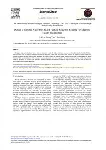
3. Proposed Methodology and Example Learning Applications 3.1. Iterative Feature Construction algorithm In this section we present our iterative feature constructor algorithm that applies mathematical operators to pairs of original features to successively create new features. The detailed algorithm is formalized in figure 1. We limit the set of operators to standard arithmetic operators, i.e., π = {+, -, *, /}. In each iteration, all possible pairs of original features are combined with each of the operators to create a set of new features. The χ2 feature selector method (Forman, 2003) is applied to the combined set of original features and the newly constructed features to rank them in their order of importance in discriminating the positive and negative examples. Only a certain number of highly ranked features from this set are then selected and the process is repeated. Note that each iteration creates terms of a higherorder polynomial. For fairness of comparison, we select the same number of features at each iteration. One could devise an appropriate stopping criteria based on the values given by the χ2 feature selector. However, we consider only the performance of the new features constructed in the first iteration. To study the effectiveness of our feature construction methodology, we compare the performance of a machine learning method on the original set of features with its performance on the new set of features. For consistency of the results we use the following three techniques that have been used extensively in machine learning and data mining applications: genetic algorithm, C4.5, and Lazy Learner. We describe each of the methods below. 3.1.1. GA In this section we present the design of a genetic algorithm (Goldberg, 1989) for rule learning in a data mining application. Assume that the data mining problem has k attributes and we have a set of training examples ψ = {(Et, c) | t = 1, …, T}, where T is the total number of examples, each example Et is a vector of k attribute values Et = [et1, et2, …, etk], and c is its classification value (usually a binary value indicating whether the example is a positive or a negative). The goal of data mining is to learn concepts that can explain or cover all of the positive examples without covering the negative examples. The representation of a concept or a classifier used by the GA is that of a disjunctive normal form. A concept is represented as Ω = δ 1 ∨ δ 2 ∨ K ∨ δ p , where each disjunct δi (also referred to as a rule) is a conjunction of conditions on the k attributes, δ i = (ξ1,i ∧ K ∧ ξ k ,i ) . In order to handle continuous attributes each condition ξj,i is in the form of a closed interval [aj, bj]. We say that a disjunct δi covers an example Et if (a j ≤ e tj ≤ b j )∀j = 1K k Each member of the population in the GA is a single disjunct and the GA tries to find the best possible disjunct. At each generation it retains the best disjunct and replaces the rest through the application of the genetic operators. After the genetic algorithm converges, the best disjunct found is retained and the positive examples it covers are removed. The process is repeated until all the positive instances are covered. The final rule or concept is then the disjunct of all the disjuncts found. The fitness function looks at the number of positive and negative examples covered by the rule but it also assigns partial credit for the number of attribute intervals on that rule that match the corresponding attribute values on a positive training example. Specifically, the fitness function is given by F = + Ck(p n), where is the total number of partial matches, C is a constant, k is the number of attributes, p is the number of positive examples covered by the rule, and n is the number of negative examples covered by the rule. 3.1.2. C4.5 C4.5 uses divide-and-conquer approach to construct decision trees (Quinlan, 1993). C4.5 extends ID3, and incorporates means to deal with missing values, real-valued attributes, pruning of decision trees, rule derivation, among others. It uses gain ratio, and information-based measure, as the default splitting criterion at the nodes. Let C denote the number of classes and p(D, j) the proportion of cases in D

that belong to the jth class. The residual uncertainty about the class to which a case in D belongs can be expressed as Info(D) = -∑j=1C p(D,j) x log2(p(D,j)) Information gain is calculated by subtracting the weighted information in the parent and children nodes created by the split. Gain(D, X) = Info(D) - ∑i=1 k (|Di| / |D| ) x Info(Di) Information Gain ratio is the information gain divided by the amount of information in the split-generated data distribution: Gain-Ratio(D,X) = Gain(D,X) / Infosplit(D,Split) where Infosplit(D,Split) = - ∑i=1k (|Di| / |D| ) x log2(|Di| / |D| ) C4.5 builds a decision tree using the standard TDIDT (top-down induction of decision trees) approach, recursively partitioning the data into smaller subsets, based on the value of an attribute. At each step in the construction of the decision tree, C4.5 selects the attribute that maximizes the information gain ratio. The induced decision tree is pruned using pessimistic error estimation since without pruning new nodes are constructed until purity (i.e., examples at every leaf node belongs to only one class). Post-pruning is done primarily to prevent over-fitting and to alleviate any effect due to noisy data. 3.1.3. Lazy Learning Eager learning methods construct a classification model based on training data set and classify test data using this model. Lazy learners, on the other hand, simply store training data with minor processing and wait till testing data arrive (e.g., Aha, 1997). Lazy learners thus spend less time and computing resources during the training phase but more during prediction using testing data. Generally speaking, lazy learners use a richer hypothesis space since they use specific local knowledge unlike eager learners that use hypotheses that cover entire instance space. Instance-based learning methods such as knearest neighbor, locally-weighted regression, and case-based reasoning store training examples and delay processing until test data arrive. Instance-based learners classify a testing instance by comparing it to a set of pre-classified training examples. The assumption here is that similar instances will have similar classifications. There are, however, several different means to measure the “similarity” of instances. There are also several different ways to classify instances. We use K*, an instance-based learner, as an example lazy learner (Cleary and Trigg, 1995). K* uses entropy as a distance measure to consistently handle symbolic and real-valued attributes as well as missing values. Cleary and Trigg (1995) compute the distance between two instances using information theory. The complexity of transforming one instance into the other is taken as the distance between them. They specifically consider Kolmogorov distance as the length of the shortest string connecting two instances. The K* distance sums over all possible transformations between two instances. The probability function P* is defined as the probability of all paths from instance a to instance b through transformations t : P*(a|b) = ∑ t(a)=bP(t) and the K* function is defined as: K*(b|a) = -log2P*(b|a). Strictly speaking, K* is not a distance function since K*(a|a) could be non-zero and K*(a|b) need not equal K*(b|a). K* also has the following properties: K*(b|a) ≥ 0; K*(c|b) + K*(b|a) ≥ K*(c|a). 3.2. Results & Discussion The methods were tested on a real world chemical process control plant data. The data we use has 30 process variables, of which only 9 are controllable, and one boolean classification variable. All variables have continuous values from the domain [0.0 0.99]. The data set has 572 instances, of which 355 are positive examples and 217 are negative examples. It was randomly broken up into 10 pairs of a training set of 344 examples and a testing set of 228 examples. Table 1 presents the prediction accuracy of the concepts learned by the three machine learning methods on the respective testing sets. As mentioned earlier we compare the performance of each method using the original set of features with their performance using the features created in the first iteration of our feature construction method. As can be seen, all the three methods improve their prediction accuracy using the new features. We also report the

results of a paired t-test for the three methods. The improvement in results produced by GA and Lazy Learner were found to be statistically significant. As an example of the concepts learned using the new features, consider the following given by the GA. On one of the data sets, the best rule learned by the GA was the following disjunct

( x7 ≤ 0.74) ∧ ( x1 ≤ 0.65) ∧ ( x 4 ≥ 0.44) ∧ ( x8 ≤ 0.52) ∧ ( x 2 ≥ 0.38)

which covered 116 positive examples together with 27 negative examples. Using the new features on the same data set, the GA learned the following disjunct:

( x1 ⋅ x5 ≤ 0.45) ∧ ( x1 + x5 ≥ 0.33) ∧ ( x1 + x7 ≤ 0.85) ∧ ( x3 + x6 ≥ 0.38)

which covered 134 positive examples together with 29 negative examples, an improvement of almost 18% in accuracy. 4. Conclusion We presented an iterative feature construction methodology that was shown to improve the prediction accuracy of three machine learning methods. Since the methodology is independent of the underlying learning algorithm, it can be used to potentially improve the performance of any learning method. Although we presented the results based on only one data set, we are currently working on applying this method on various real world data sets. We are also investigating whether this method can iteratively construct complex functions from synthetic data created from those functions. Finally, we are investigating various stopping criteria that the feature constructor can use in deciding when to stop creating new features. References Aha, David. (1997) “Lazy Learning,” Artificial Intelligence Review, 11, 7-10. Bloedorn, Eric, and Ryszard S. Michalski. (1998). “Data-Driven Constructive Induction,” IEEE Intelligent Systems, 30-37.

Cleary, John, G. and Leonard, E. Trigg. (1995) "K*: An Instance- based Learner Using an Entropic Distance Measure", Proceedings of the 12th International Conference on Machine learning, 108-114. Flach, Peter A., and N. Lachiche. (2001). “Confirmation-guided discovery of first-order rules with tertius.” Machine Learning, 42, 61–95. Flach, Peter A., and Nada Lavrac (2000). “The Role of Feature Construction in Inductive Rule Learning,” Proc. of the Intl Conf on Machine Learning 2000 Workshop on Attribute-Value and Relational Learning: Crossing the Boundaries, 1-11. Forman, G. (2003). "An Extensive Empirical Study of Feature Selection Metrics for Text Classification," Journal of Machine Learning Research, 3, 1289-1305.

Goldberg, D. Genetic Algorithms in Search, Optimization and Machine Learning. 1989. Reading, MA: Addison-Wesley Publishing Co., Inc Klösgen, W. (1996). “Explora: A multipattern and multistrategy discovery assistant.” In U. M. Fayyad, G. Piatetsky-Shapiro, P. Smyth, & R. Uthurusamy (Eds.), Advances in knowledge discovery and data mining, 249–271, Menlo Park, CA: AAAI Press. Langley, P., Zytkow, J. M., Simon, H. A., & Bradshaw, G. L. (1986). “The search for regularity: Four aspects of scientific discovery.” Machine learning: An artificial intelligence approach, 2, 425– 470, Los Altos, CA: Morgan Kaufmann.

Matheus, Christopher J., and Larry Rendell. (1989) “Constructive induction in decision trees.” Proceedings of the Eleventh IJCAI, 645–650. Pagallo, G. (1989). “Learning DNF by decision trees.” Proceedings of the Eleventh IJCAI, 639–644. Quinlan, J. R. (1986). “Induction of decision trees.” Machine Learning, 1(1), 81–106. Quinlan, J. R. (1993). C4.5: Programs for Machine Learning. Morgan Kaufmann Publishers. Utgoff, Paul E. (2001). “Feature Construction for Game Playing,” in Fuerenkranz and Kubat (eds.)

Machines that Learn to Play Games, 131-152, Nova Science Publishers. Vilalta, Ricardo, and Larry Rendell. (1997). “Integrating Feature Construction with Multiple Classifiers in Decision Tree Induction,” Proceedings of International Conference on Machine Learning, 394402, Morgan-Kaufman. Wrobel, S. (1997). “An algorithm for multi-relational discovery of subgroups.” Proceedings of the first European symposium on principles of data mining and knowledge discovery. Berlin: Springer. Yang, D.-S., Larry Rendell, and Gunnar Blix. (1991). “A scheme for feature construction and a comparison of empirical methods.” Proceedings of the Twelfth IJCAI, 699–704. Data Set 1 2 3 4 5 6 7 8 9 10 Avg. Std. Dev. Paired t-test

GA Base 78.07% 82.46% 81.14% 77.63% 85.53% 80.70% 79.39% 79.39% 83.33%

C4.5

Level1 FC 80.70% 79.39% 80.26% 81.14% 87.28% 85.97% 80.26% 82.46% 79.83%

Base 78.95% 86.84% 81.14% 82.02% 90.79% 82.90% 82.46% 84.65% 83.77%

Level1 FC 82.02% 87.72% 82.46% 83.33% 85.09% 84.65% 80.26% 87.28% 82.46%

Lazy Learner Base 82.89% 90.35% 85.53% 86.40% 87.28% 85.53% 87.72% 86.40% 84.21%

Level1 FC 83.77% 88.59% 85.53% 86.40% 90.79% 88.59% 86.84% 89.03% 88.15%

79.39% 83.77% 84.21% 85.97% 89.90% 89.03% 80.70% 82.11% 83.77% 84.12% 86.62% 87.67% 0.02

0.03 0.09

0.03

0.02 n.s.

0.02

0.02 0.07

Table 1. Prediction accuracy results for the 3 ML methods

Begin let ∆ = set of n original features let π = set of m operators let FCπ(∆) = set of m n C 2 new features constructed by applying π over ∆. let χ2(∆) = ordered set of features ∆ resulting from χ2 feature selector repeat ∆’ = ∆ ∪ FCπ(∆) ∆’ = χ2(∆’) ∆ = set of best n features from ∆’ until (the stopping criteria is met) use an ML algorithm to learn a concept using the new features in ∆ End Figure 1. The proposed iterative feature construction algorithm