Genetic Algorithm Based Feature Selection for Speaker Trait Classification. Dongrui Wu. Machine Learning Lab, GE Global
Genetic Algorithm Based Feature Selection for Speaker Trait Classification Dongrui Wu Machine Learning Lab, GE Global Research, Niskayuna, NY USA
[email protected]
Abstract Personality, likability, and pathology are important speaker traits that convey rich information beyond the actual language. They have promising applications in human-machine interaction, health informatics, and surveillance. However, they are less researched than other paralinguistics phenomena such as emotion, age and gender. In this paper we propose a novel feature selection approach for speaker trait classification from a large number of acoustic features. It combines Fisher Information Metric feature filtering and Genetic Algorithm based feature selection, and fuses several elementary Support Vector Machines with different feature subsets to achieve robust classification performance. Experiments on an INTERSPEECH 2012 Speaker Trait Challenge dataset show that our approach outperforms both baseline approaches. Index Terms: Paralinguistics, Speaker Trait Classification, Personality, Likability, Pathology, Genetic algorithm, Fisher Information Metric, SVM
1. Introduction Speaker states and traits, including emotion, age, gender, sleepiness, intoxication, personality, likability, pathology, etc, are important phenomena in paralinguistics. They convey rich information beyond the language itself. Among them, personality, likability and pathology are less researched speaker traits. However, they have important applications in human-machine interaction [1], health informatics, and surveillance. The INTERSPEECH 2012 Speaker Trait Challenge [2] is organized to fill this gap. Three sub-challenges are addressed: 1. Personality Sub-Challenge, in which the personality of a speaker has to be determined based on acoustic features. The personality is represented by the 5-dimension OCEAN (Openness to experience, Conscientiousness, Extraversion, Agreeableness, and Neuroticism) model [3]. Each dimension is discretized into two levels: below average, or above. 2. Likability Sub-Challenge, in which the likability of a speaker’s voice has to be determined based on
acoustic features. The likability is discretized into two levels: below average, or above. 3. Pathology Sub-Challenge, in which the intelligibility of a speaker has to be determined based on acoustic features. Again, the intelligibility is discretized into two levels: below the median, or above. 6125 acoustic features were extracted for each speaker in each sub-challenge. More descriptions about the data and features can be found in [2]. This paper proposes a novel Genetic Algorithm (GA) based feature selection method for speaker trait classification and achieves better performance than the two baseline approaches. The details of the algorithm are presented in Section 2. The experimental results are given in Section 3.
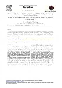
2. The Proposed Algorithm The flowchart of our algorithm is shown in Fig. 1. Linear Support Vector Machines (SVMs), implemented by the libSVM [4], are used as our classifier. We first normalize each feature to [0, 1], then perform feature filtering by the Fisher Information Metric and feature selection by GA. Next we optimize the parameters of the SVMs and finally fuse several of them for robust performance. More details on these steps are described next. 2.1. Data Normalization Data normalization is used to avoid attributes in larger numerical ranges dominating those in smaller ranges, and to avoid numerical difficulties during the calculation. It is a recommended step in libSVM [4]. In this paper we perform feature data normalization before feature filtering and selection. We combine all examples from the training, development and test datasets and normalize each feature into [0, 1]. 2.2. Feature Filtering by Fisher Information Metric There is a total of 6125 features. Not all of them are equally useful in classification. The useless or less useful features should be removed as they increase the computational cost and also deteriorate the classification perfor-
popular global optimization method, to determine which features should be selected. The flowchart of the GA is shown in Fig. 2. 20 generations were used and there were 100 chromosomes in each generation. In the following we use N = 100 as an example to explain how each step works.
Data Normalization Each feature in [0, 1]
Feature Selection by Fisher Information Metric 2000 features
Initial population Feature Selection by GA, N=100 100 features
.. .. .. ...
SVM Parameter Optimization
Feature Selection by GA, N=500
Fitness computation
500 features
Reproduction
SVM Parameter Optimization
Optimal SVM
Optimal SVM
SVM Fusion
Crossover Mutation
Final classifier
Terminate?
Figure 1: Flowchart of our algorithm.
Yes
mance. The feature selection procedure consists of two steps. The Fisher Information Metric, which is a measure of the distinguishing power of a single feature, is used in feature filtering. We consider each feature independently and compute its Fisher information metric. Let N0 be the number of negative training examples, N1 be the number n=1,...,N0 +N1 of positive training examples, and {xni }i=1,...,6125 be the values of the ith feature. Then, the Fisher information metric for two-class classification is computed as [5]: Fi =
(m0 − m1 )2 , σ0 + σ1
i = 1, ..., 6125
No
(1)
where m0 (m1 ) is the mean of xni corresponding to the negative (positive) training examples, and σ0 (σ1 ) is the variance of xni corresponding to the negative (positive) training examples. We then sort {Fi }i=1,...,6125 in descending order and pick only the top M features in further feature selection. M = 2000 was used in our experiment. It was chosen empirically. 2.3. Feature Selection by Genetic Algorithm Two questions need to be addressed in further feature selection: 1) How many features should be used? and, 2) Which features should be selected? As it is difficult to determine how many features should be used, we address the first question by selecting a group of features with different lengths (N = {100, 200, 300, 400, 500} were used in this paper) and then fusing the corresponding SVM classifier for robust performance. Given a target N, the number of features to be selected, we use GA [6], a very
Output the chromosome with the maximum fitness
Figure 2: Flowchart of the GA.
2.3.1. Initial Population Each chromosome in the initial population contains the indices of 100 random features selected from the 2000 features, and the initial population has 100 such chromosomes. The most intuitive way to generate a chromosome is to generate 100 random integers in [1, 2000]. However, there may be duplicate indices, especially when N gets large. So, we need to check each chromosome and replace duplicate indices by new indices to ensure all 100 indices in a chromosome are unique. 2.3.2. Fitness Evaluation The fitness of each chromosome is evaluated using both the training dataset and the development dataset. For the training dataset, we use 5-fold cross-validation and SVM to compute the unweighted average (UA) recall (ai , where i is the index of the chromosome). For the development dataset, we first train a SVM using the entire training dataset, and then compute the UA (bi ) on the development dataset. The overall fitness of the ith chromosome is then computed as fi = (ai + w · bi )/(1 + w),
i = 1, ..., N
(2)
where w is a constant to ensure that ai ≈ bi . w = 1.5 was used in our experiment and it was chosen empirically.
2.3.3. Reproduction In reproduction, we copy the 100 chromosomes in the previous generation directly to the next generation. The top five chromosomes with the maximum fitness are not touched at all. The rest 95 chromosomes are modified using crossover and mutation. 2.3.4. Crossover To perform crossover, we need to find a partner for each of the 95 chromosomes. Every chromosome in the 100chromosome population has a probability to be selected, and the probability is proportional to fi2 [ fi is defined in (2)]. We used fi2 instead of fi for faster convergence. Once the partner of a chromosome is identified, the two chromosomes perform crossover at a random location to obtain a new chromosome, which is stored in the next generation. 2.3.5. Mutation We do not perform mutation explicitly. However, the new chromosome obtained from the crossover of two parent chromosomes usually has some duplicate indices. We replace these duplicates by randomly generated unique indices, which is equivalent to mutation. 2.4. SVM Parameter Optimization In the above GA-based feature selection, the complexity parameter C of the linear SVM is fixed to be 0.1. However, this may not be optimal. When the GA terminates after 20 generations, we select the top 10 chromosomes in the final population with the maximum fitness. For each of them, we test C ∈ {10−4, 10−3.8, ..., 100 } and record the C which gives the maximum fitness. In this way we obtain the optimal C for each of these top 10 chromosomes. The best chromosome is then chosen as the one which gives the best fitness among them. The 100 indices stored in that chromosome constitute our best feature subset for N = 100. 2.5. SVM Fusion We repeat the above feature selection by GA and SVM parameter optimization for N = {100, 200, 300, 400, 500} to obtain five best feature subsets with different length, and the corresponding C. These can be used to construct
five different SVMs. We then use a majority vote to fuse them for robust performance.
3. Experimental Results The Fisher Information Metrics for the 6125 features are shown in Fig. 3. Observe that only a very small portion of the 6125 features have good distinguishing ability. Removing the less useful features can increase the speed and robustness of our algorithm. 0.09
Fisher Information Metric
We need to point out that in each generation, the partition of the five folds in 5-fold cross-validation is generated randomly, i.e., the five folds in each generation are different from those in other generations. We believe this can increase the generability of the resulting feature subset because it is extensively validated in many different scenarios. However, more experiments are needed to verify this conjecture.
0.08 0.07 0.06 0.05 0.04 0.03 0.02 0.01 1000
2000
3000
4000
5000
6000
Feature index
Figure 3: Fisher Information Metrics for different features. Note that the metrics have been sorted in descending order. The first 2000 features were used in this paper. The UAs on the training and development datasets in each GA generation are shown in Fig. 4, as well as the aggregated UA by (2). Observe from Fig. 4(c) that the sum of the UAs on the training dataset and the development dataset, which was used as the fitness measure in our experiment, generally increases with the number of generations. However, there are fluctuations, because in each generation the partition of the five folds in evaluating the training performance was different. There will be less fluctuations when the number of folds is larger, at the cost of increased computation time. We use the five feature subsets and C obtained after SVM parameter optimization to train five SVM model based on both the training and development datasets, compute their classification results individually for the test dataset, and then fuse them to obtain the final classification for the test dataset. The UAs and weighted averages (WAs) are shown in Table 1. For comparison purpose the baseline results using SVM and Random Forests (RF), given in [2], are also shown. Due to time constraint we have only finished our experiments on the Likability dataset, but in the final submission we will report results on all three sub-challenges. Observe that: 1. Our UA and WA on the development dataset are significantly better than those in the baseline SVM and RF approaches. This is because we considered the development dataset explicitly in GA-based feature selection, at the risk of overfitting.
2. Our UA and WA on the test dataset are considerably better than the UA and WA in the baseline SVM approach, and are also slightly better than the UA and WA in the baseline RF approach.
0.71
CV UA on training dataset
0.7 0.69
3. Our UA and WA on the test dataset are much lower than those on the development dataset, because of overfitting. This implies that there is great room for improvement. How to reduce this overfitting will be considered in our future study.
0.68 0.67 0.66 0.65 0.64 N=100 N=200 N=300 N=400 N=500
0.63 0.62 2
4
6
8
10
12
14
16
18
20
Table 1: Likability classification results. The values shown are percentages.
Generation
Task
(a)
Likability
0.67
Classifier Baseline SVM Baseline RF Our algorithm
Development UA WA 58.5 58.4 57.6 57.5 68.6 69.1
Test UA WA 55.9 56.1 59.0 59.2 59.5 59.6
UA on development dataset
0.66
0.65
4. Conclusions
0.64
0.63
0.62 N=100 N=200 N=300 N=400 N=500
0.61
2
4
6
8
10
12
14
16
18
20
Generation
Sum of UA on training and development datasets
(b) 0.675 0.67 0.665
Personality, likability, and pathology are important speaker traits which have promising applications in human-machine interaction, health informatics, and surveillance; however, they are less researched than other paralinguistics phenomena such as emotion, age and gender. In this paper we have proposed a novel feature selection approach for speaker trait classification from a large number of acoustic features. It combines Fisher Information Metric feature filtering and GA-based feature selection, and fuses several elementary SVMs with different feature subsets to achieve robust classification performance. Experiments on an INTERSPEECH 2012 Speaker Trait Challenge dataset showed that our approach can outperform both baseline approaches.
5. References
0.66
[1] F. Metze, A. Black, and T. Polzehl, “A review of personality in voice-based man machine interaction,” in Proc. HCI International, vol. 2, Orlando, FL, July 2011, pp. 358–367.
0.655 0.65 0.645 N=100 N=200 N=300 N=400 N=500
0.64 0.635 2
4
6
8
10
12
14
16
18
20
Generation
(c)
Figure 4: The UAs in different generations of the GA. (a) The UA from the 5-fold cross-validation on the training dataset; (b) The UA on the development dataset; (c) The sum of UAs on the training dataset and the development dataset.
[2] B. Schuller, S. Steidl, A. Batliner, E. Noth, A. Vinciarelli, F. Burkhardt, R. van Son, F. Weninger, F. Eyben, T. Bocklet, G. Mohammadi, and B. Weiss, “The Interspeech 2012 Speaker Trait Challenge,” in Proc. Interspeech 2012, Portland, OR, September 2012. [3] J. S. Wiggins, Ed., The five-factor model of personality: Theoretical perspectives. NY: Guilford, 1996. [4] C.-C. Chang and C.-J. Lin, “LIBSVM: A library for support vector machines,” 2009. [Online]. Available: http://www.csie.ntu.edu.tw/˜cjlin/libsvm. [5] R. O. Duda, P. E. Hart, and D. G. Stork, Pattern Classification. NY: Wiley-Interscience, 2000. [6] D. E. Goldberg, Genetic Algorithms in Search, Optimization and Machine Learning. Addison-Wesley, 1989.