Genetic algorithm full-waveform inversion: uncertainty estimation and ...

Bollettino di Geofisica Teorica ed Applicata

Vol. 58, n. 4, pp. 395-414; December 2017

DOI 10.4430/bgta0199

Genetic algorithm full-waveform inversion: uncertainty estimation and validation of the results A. Sajeva, M. Aleardi and A. Mazzotti Earth Sciences Department, University of Pisa, Italy (Received: January 31, 2017; accepted: July 5, 2017)

ABSTRACT

We cast the genetic algorithm-full waveform inversion (GA-FWI) in a probabilistic framework that through a multi-step procedure, allows us to estimate the posterior probability distribution (PPD) in model space. Since GA is not a Markov chain Monte Carlo method, it is necessary to refine the PPD estimated by GA (GA PPD) via a resampling of the model space with a Gibbs sampler (GS), thus obtaining the GA+GS PPDs. We apply this procedure to two acoustic 2D models, an inclusion model and the Marmousi model, and we find a good agreement between the derived PPDs and the varying resolution due to changes in the seismic illumination. Finally, we randomly extract several models from the so derived PPDs to start many local full-waveform inversions (LFWIs), which produce final high-resolution models. This set of models is then used to numerically estimate the final uncertainty (GA+GS+LFWI PPD). The multimodal and wide PPDs derived from the GA optimization, become unimodal and narrower after LFWI and, in the well illuminated parts of the subsurface, the final GA+GS+LFWI PPDs contain the true model parameters. This confirms the ability of the GA optimization in finding a velocity model suitable as input to LFWI.

Key words: genetic algorithm, Gibbs sampler, full waveform inversion, uncertainty estimation.

1. Introduction Full-waveform inversion (FWI) is an optimization procedure for seismic data sets that is based on an accurate numerical simulation of the equations of motion and on an iterative procedure to fit the waveforms of simulated and observed data (Virieux and Operto, 2009; Sirgue et al., 2010; Prieux et al., 2011; Morgan et al., 2013). FWI proved to be a valuable tool to derive highresolution quantitative models of the subsurface. In the simplest FWI implementation the Earth is regarded as an isotropic and acoustic medium. Other approximations, such as elastic, viscoelastic, and anisotropic have been proposed to treat complex subsurface models that require more accurate simulations of the wave propagation (Operto et al., 2013). The most common numerical method to simulate the wavefield is the finite-difference method; other approaches are the finite element methods or the spectral methods (Fichtner, 2010). Full-waveform inversion is a strongly non-linear and multidimensional inverse problem, which involves hundreds or even thousands of unknown model parameters, and is characterised by a multi-modal cost function. This inverse problem is usually solved in the framework of the acoustic approximation applying a local linearization of the forward modelling (based on the © 2017 – OGS

395

Boll. Geof. Teor. Appl., 58, 395-414

Sajeva et al.

steepest descent or conjugate gradient algorithms). Local methods can efficiently optimize a large number of unknown model parameters, whereas the limitation of describing the subsurface as an acoustic model is needed to reduce the computational cost, the non-linearity and the illposedness of the inverse problem (Operto et al., 2013). From these considerations, it emerges that local FWI (LFWI) is subjected to fall into local minima of the cost function in case of lack of low frequencies, lack of large source-receiver offsets, highly-complex media, or a poor starting model. In particular, several methods have been proposed to make the LFWI result less affected by the choice of the starting model (Bunks et al., 1995; Diouane et al., 2014; Tognarelli et al., 2015, 2016; Sajeva et al., 2016). In addition, local FWI is generally cast in the framework of deterministic approaches. This means that a single best-fitting model is provided and any information on the associated uncertainties is discarded. This approach has been generally followed for the sake of pragmatism and computational feasibility because of the large number of unknowns that are involved in a FWI (Fichtner, 2010). Nevertheless, the computational power of CPUs and GPUs is continuously increasing and new larger and more powerful clusters that efficiently distribute the cost of large problems are designed. This progressively moves forward the threshold of what is feasible and unfeasible. Moreover, FWI is a strongly ill-conditioned inverse problem in the sense that many solutions explain the observation equally well. Hence, it is more appropriate to appraise a region of acceptable solutions above a certain threshold, that is the “equivalence region of solutions” (Fernández Martinez et al., 2012), instead of providing a single best-fitting solution. In other words, the estimation of the uncertainties affecting the final result of LFWI, in the form of the posterior probability distribution (PPD) in the model space, can provide valuable insights on the problem itself and on the capability of FWI to determine the subsurface characteristics. Stochastic global optimization methods [i.e., genetic algorithms (GAs), simulated annealing, particle swarm, neighbourhood algorithm, differential evolution] offer another possible approach to tackle the FWI problem. From one hand, these methods can efficiently explore the entire model space, thus reducing the risk of falling into local minima of the cost function. From the other hand, the stochastic approach makes it feasible to cast the FWI in a probabilistic framework. Stochastic FWI was first performed by Sen and Stoffa (1991, 1992) for problems with a limited number of unknowns and in which a 1D subsurface model was assumed. Other noteworthy applications of stochastic FWI can be found in Mallick (1999), Mallick and Dutta (2002), Mallick et al. (2010), Fliedner et al. (2012), and Li and Mallick (2015). The main problem to be addressed in stochastic FWI is the high computational cost that increases exponentially with the number of unknowns. This scaling problem [sometimes referred to as the “curse of dimensionality”: Bellman (1957)] makes the stochastic approach to FWI often unfeasible for 2D or 3D applications. Nevertheless, due to the recent growth of high-performance computing, stochastic FWI begins to be used to derive low-resolution 2D compressional velocity models that, if needed, can be used as starting models for local FWI (Gao et al., 2014; Datta and Sen, 2016; Sajeva et al., 2016; Tognarelli et al., 2016). Regarding this last point, this work aims to demonstrate that a GA optimization can provide a velocity model suitable as input to local FWI. To this end, we cast the FWI in a probabilistic framework by combining the stochastic FWI method proposed by Sajeva et al. (2016) with the hybrid method for uncertainty estimation in 1D elastic FWI proposed by Aleardi and Mazzotti (2017). In particular, the FWI algorithm implemented by Sajeva et al. (2016) is aimed at deriving a low-resolution velocity model and is based on a GA-driven optimization 396

Genetic algorithm full-waveform inversion

Boll. Geof. Teor. Appl., 58, 395-414

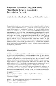
procedure. The authors used this particular stochastic method because GAs often display the best scaling with the number of model parameters and outperform other well-known stochastic methods (such as particle swarm optimization, adaptive simulated annealing or neighbourhood algorithm) in finding the global minimum of several different cost functions (Sajeva et al., 2014, 2017). Other applications of GAs in solving a geophysical optimization problems can be found in Sen and Stoffa (2013), Aleardi (2015), Aleardi et al. (2016), Aleardi and Ciabarri (2017), and Pafeng et al. (2017). However, GAs are not a Markov-Chain Monte Carlo (MCMC) method (Rubinstein and Kroese, 2011) and, as a consequence, they offer a biased estimate of the posterior probability distributions (PPDs) of model parameters. To overcome this limitation and to derive a reliable estimate of uncertainties, many strategies can be followed. In this work, we follow the line of Sambridge (1999) who combined a stochastic optimization with a subsequent resampling of the model space according to a MCMC method known as the Gibbs sampler [GS: Geman and Geman (1984)]. Sambridge (1999) applied this method in a seismological problem concerning the inversion of receiver functions in which the neighbourhood algorithm was used to optimize a limited number of unknowns (24). Successively, Aleardi and Mazzotti (2017) applied this hybrid method for uncertainty estimation to the 1D elastic FWI, with a larger number of unknown model parameters (tens of unknowns) and using a GAs-driven optimization. Here, this uncertainty estimation procedure is extended and adapted to the context of local and acoustic 2D FWI. The paper is organized as follows. We start with a brief description of the workflow of our approach to FWI which comprehends a global method (GA), a resampling method (Gibbs sampler), and a local method (steepest descent). Next, we shortly present the criteria to determine the sparse grid points for the global method. Finally, we discuss the application of the complete workflow to two synthetic cases. The first example is the inversion of a simple inclusion model, which is a variation of the model studied in Mora (1989), whereas in the second example we apply our method to the more complex Marmousi model. A detailed mathematical description of the method is given in Appendix. 2. The method In this section, we give a schematic and qualitative description of the workflow we use to estimate uncertainty in FWI. Additional details are given in Appendix. Our method is schematically outlined by the diagram represented in Fig. 1. In the first step, given an a priori information on the model parameters (prior model), we employ a real-valued GA to perform a global inversion with the aim of collecting all the explored low-resolution models (ensemble of GA models), from which we also extract the best-fitting model. The GAs are a class of randomized search methods that can be applied to large-scale optimization problems. They treat models collectively, such that the ensemble of models (or population) evolves toward new generations with lower misfit by means of selection, recombination, and mutation (Goldberg, 1989; Mitchell, 1998; Sivanandam and Deepa, 2008). Additional details about the GA implementation we use are given in Sajeva et al. (2016). After this step, by exploiting the entire ensemble of models sampled by GAs, we can obtain a rough and biased uncertainty estimation. We name this probability distribution the GA PPD. In the second step, the entire ensemble of GA models is appraised following the procedure of Sambridge (1999), which consists in an importance sampling of the model space explored by GAs 397

Boll. Geof. Teor. Appl., 58, 395-414

Sajeva et al.

Fig. 1 - Schematic representation of the procedure.

using the GS. The model space is divided into Voronoi cells, each one associated with a single GA model and its likelihood. This creates a multi-dimensional interpolant which is resampled by the GS algorithm. This step yields a non-biased PPD (that we call the GA+GS PPD) which expresses the uncertainties affecting the best-fitting GA model. It is crucial to note that no additional forward modelling is needed in the GS step. This characteristic is important because it determines the low computational cost, and then the feasibility, of this model-space resampling. The third step consists in extracting a sufficiently large set of models from this estimated PPD, by means of a MCMC algorithm. Each one of these models is used as starting model for a local FWI that constitutes the fourth step of our procedure. Finally, the last step applies a non-parametric method (i.e., the kernel density estimation) to the ensemble of models resulting from LFWI to derive the final PPDs, e.g., the 1D marginal PPD for each model parameter. We name this final probability distribution the GA+GS+LFWI PPD. 3. Model parameterization for the GA optimization A peculiar aspect of the GA optimization we emphasize here, is the choice of the model parameterization. As said before, in a global optimization procedure it is crucial to reduce the number of unknowns. To this end, we reduce the number of model parameters by resampling the prior model onto an irregular grid with cell sizes chosen according to seismic resolution criteria, that is, proportional to a quarter of the dominant wavelength for the vertical resolution, δv, and proportional to the first Fresnel zone for the horizontal resolution, δh (1) (2) where λ is the dominant wavelength of the seismic wave, V is the interval velocity of the layer, f is the dominant frequency of the seismic wave, and z is the reflector depth. Let us focus on the case where V changes only with depth (1D velocity profile). In this case both δh and δv are functions of the sole depth. Hence, starting from the first depth, z0, for which the exact velocity is unknown (e.g., the surface or the water bottom), we resample the prior model at depths: 398

Genetic algorithm full-waveform inversion

Boll. Geof. Teor. Appl., 58, 395-414

(3) where a is a real scale factor, and N is such that zN is less than the maximum depth of the model. Analogously, we use the horizontal resolution to resample the horizontal coordinates. The horizontal step size, ΔX, at each depth zn is: (4) 4. First synthetic example: the inclusion model We first apply the method to an acoustic inclusion model similar to the one introduced by Mora (1989). This model is constituted by a spherical homogenous inclusion in a background velocity characterized by a constant gradient with depth and a deep reflection (Fig. 2a). For the forward modelling, we use the finite-difference method, with accuracy of second order in time and fourth order in space, a vertical and horizontal space step of 48 m, a time step of 4 ms, and a Ricker wavelet as the source signature. The acquisition geometry consists of 31 sources and 127 receivers all equally spaced at the surface, and, for each shot, one source illuminates all the receivers. To

Fig. 2 - a) The true model for the inclusion example; b) the centre of the ranges as a 2D colour image superimposed with the position of the irregular grid nodes at which the Vp values are optimized during the GA inversion; c) ranges of admissible values for Vp during the GA inversions are between the min (blue) and max (red) curves; d) the final bestfitting model after the GA optimization.

399

Boll. Geof. Teor. Appl., 58, 395-414

Sajeva et al.

Fig. 3 - a) The observed first shot, filtered below 6 Hz; b) the corresponding predicted shot after the GA optimization and low-pass filtering; c) the differences between (a) and (b).

evaluate the misfit, we use the L2 norm applied to a low-pass filtered (with a maximum frequency around 6 Hz) and a trace-by-trace normalized version of the data. As prior information, we use a simple 1D P-wave velocity (Vp) model with velocity linearly increasing with depth from 1500 to 3000 m/s. This model is used to centre the GA inversion ranges and to build the irregular GA grid with the procedure described in the previous section. The resulting grid and the linear 1D model are shown in Fig. 2b. This grid has 24 nodes. These nodes are bilinearly interpolated to the finite-difference grid for the forward-modelling. The range of admissible values for the model parameters investigated during the GA inversion is limited by the min and max curves of Fig. 2c. In the GA inversion, we performed 16,000 model evaluations and the final best-fitting model is shown in Fig. 2d. This result may be considered a good macro model, since it contains the long-wavelengths of the true model. The quality of the result can be assessed also by observing the seismic data error. Fig. 3 shows: a) the observed leftmost shot filtered below 6 Hz; b) the corresponding predicted shot, and c) the differences between (a) and (b). Note the fair match between the observed and predicted data. In fact, even though some reflections are unpredicted and the correct amplitudes of the events are sometimes mispredicted, the overall energy of the waveform differences is small. We now appraise the entire ensemble of GA models to quantify the uncertainty affecting the GA solution of Fig. 2d. Figs. 4 and 5 show some example of marginal GA PPDs and GA+GS PPDs computed for six different positions (cells) in the model. Note that, moving from the centre to the lateral edges of the model, the PPDs become broader and multimodal (Fig. 4). Analogously, moving from the top to the bottom of the model, the PPDs suffer multimodality and widening (Fig. 5). These characteristics agree with the expected loss of information due to the poorer illumination at the lateral and deep parts of the model. In addition, note that the GA PPDs usually tend to underestimate the true uncertainty, while the GA+GS probability distributions offer a more reliable estimate of the errors affecting the model parameters. 400

Genetic algorithm full-waveform inversion

Boll. Geof. Teor. Appl., 58, 395-414

Fig. 4 - a) The true model in which the coloured dots indicate the spatial position of the cells whose uncertainty is analyzed in (b) and (c); b) GA PPDs for the three cells shown in (a); c) GA+GS probability distribution for the three cells shown in (a). In (b) and (c) the red dashed lines indicate the best GA model. Note that the uncertainty increases moving from the centre to the later edges of the model and that the GA PPD underestimates the uncertainties affecting the model parameters.

Next, we use a MCMC algorithm to extract 200 models from the GA+GS PPD and we employ them as starting models for LFWI, we use the time-domain steepest-descent method, with 5 iterations at 4, 5, 6, 8, and 10 Hz. The mean value of all the resulting final models is displayed in Fig. 6a and it can be directly compared with the true model of Fig. 1a, finding a satisfactory

Fig. 5 - a) The true model in which the coloured dots indicate the spatial position of the cells whose uncertainty is analyzed in (b) and (c); b) GA PPDs for the three cells shown in (a); c) GA+GS probability distribution for the three cells shown in (a). Note that the uncertainty increases moving from the shallow to the deeper part of the model and that the GA PPD underestimates the uncertainties affecting the model parameters.

401

Boll. Geof. Teor. Appl., 58, 395-414

Sajeva et al.

Fig. 6 - a) The mean model of the set of final models (after GA+GS+LFWI); b) the 99% confidence interval of the set of final models; c) the L1-norm model error.

match. Fig. 6b shows the approximate 99% confidence interval of the set of final models that can be compared with the L1-norm model error shown in Fig. 6c. Note that the highest uncertainties are mainly localized where seismic illumination is poorer. Fig. 7 displays the observed first shot, the corresponding predicted shot after the GA+LFWI optimization and their differences. Comparing this image with Fig. 3 evidences the improved prediction. Note also that the higher frequencies have been incorporated in the fitting procedure. Figs. 8 and 9 show the 1D marginal PPDs computed after the LFWI step, at the same cell positions

Fig. 7 - a) The observed first shot; b) the corresponding predicted shot after the GA+LFWI optimization; c) the differences between (a) and (b).

402

Genetic algorithm full-waveform inversion

Boll. Geof. Teor. Appl., 58, 395-414

Fig. 8 - Final GA+GS+LFWI uncertainties estimated for three different cells located in the shallow part of the model and whose positions are indicated by the coloured dots in Fig. 4a. The red dashed lines indicate the estimated model parameters by the LFWI, whereas the green dashed lines show the true values.

indicated in Figs. 4 and 5. Again, note the loss of resolution from the centre to the lateral edges, and from the shallowest to the deepest parts of the model. Comparing Figs. 8 with 4c and Figs. 9 with 5c, it can be noted that the marginal GA+GS+LFWI PPDs do not display multimodal shapes, thus demonstrating that the whole set of starting models converge toward the same model-space region, and that, where the model is sufficiently illuminated by the wave-fronts, the true Vp values lie within the final PPDs.

Fig. 9 - Final GA+GS+LFWI uncertainties estimated for three different cells located at the centre of the model and whose positions are indicated by the coloured dots in Fig. 5a. The red dashed lines indicate the estimated model parameters by the LFWI, whereas the green dashed lines show the true parameter values.

We also show three velocity profiles (Fig. 10) from the far left to the centre of the model (at offsets 0, 2000, and 4500 m); the set of starting models is displayed by the grey beam, the set of final models is displayed by the cyan beam and the true model by the black line. These velocity profiles and the direct comparison between the GA+GS and GA+GS+LFWI probability distributions highlight several points: 1) the set of models (grey beam) resulting from GA FWI fairly reconstructs the low-frequency trend of the true velocity model; 2) the loss of resolution with depth and near the edges of both the GA and LFWI solutions; 3) the narrowing of the distributions after local FWI, and 4) the improvement in the estimation of the true model after local FWI, especially for the central part of the model where the seismic illumination is higher. These results confirm the capability of the GA optimization in finding a good initial model for LFWI, that is, a model not affected by the cycle-skipping phenomenon. 5. Second synthetic example: the Marmousi model For a second and more challenging test, we apply the proposed method to the acoustic Marmousi model (Fig. 11a). For the forward modelling, the acquisition geometry, and misfit function we use 403

Boll. Geof. Teor. Appl., 58, 395-414

Sajeva et al.

Fig. 10 - a) The true model in which the coloured lines indicate the spatial position of the Vp profiles analysed in (b); b) vertical Vp profiles for three horizontal positions. The black lines indicate the true model, the grey beams show the set of 200 starting models, and the cyan beams correspond to the set of 200 models resulting from local FWI. Note that in the leftmost plot of Fig. 10b the ensembles of initial and final velocity models are overlapped due to the poor seismic illumination at the lateral edges of the model.

the same implementation of the previous test. Recall that we low-pass filter (below 6 Hz) and trace-by-trace normalize the data prior to the misfit computation. We use a simple 1D Vp model (Fig. 11b), which constitutes our prior information, to build the irregular GA grid according to seismic resolution criteria as outlined in a previous section. The resulting coordinates for the model parameters are superimposed over the model and are depicted with red dots (Fig. 11b). The total number of unknowns for this example is 143. The ranges for the Vp values during the GA inversion are shown in Fig. 11c. As in the previous example, we use ranges that become wider with depth. In the GA inversion, we performed 40,500 model evaluations and the final best-fitting model is shown in Fig. 11d. Even in this challenging test the GA optimization has been able to estimate a subsurface macro model that contains the longwavelengths of the Marmousi model (which is shown in Fig. 11a). Fig. 12 provides us insights on the seismic data: (a) shows the observed leftmost shot lowfiltered at 6 Hz; (b) shows the corresponding predicted data, and (c) their differences. Note that (c) mainly contains unpredicted reflections and diffractions. As in the first synthetic example the next step is to quantify the uncertainty affecting the solution of Fig. 11d. To this end, we first estimate the GA PPD by exploiting the entire set of GA-sampled models. Then, we appraise this ensemble of models by means of the GS in order to obtain more reliable uncertainty estimations. Figs. 13 and 14 show some 1D marginal PPDs estimated in different cells (parts) of the model. In Fig. 404

Genetic algorithm full-waveform inversion

Boll. Geof. Teor. Appl., 58, 395-414

Fig. 11 - a) The Marmousi model; b) the 1D model that is the centre of the GA ranges superimposed with the nodes of the coarse grid (red dots). Note that the coarse grid sampling gets wider at depth; c) the range of Vp values for the GA inversion; (d) the final best-fitting model after the GA inversion.

Fig. 12 - a) The observed first shot filtered below 6 Hz; b) the corresponding predicted shot after the GA optimization and filtering; c) the differences between (a) and (b).

405

Boll. Geof. Teor. Appl., 58, 395-414

Sajeva et al.

Fig. 13 - a) The true model in which the coloured dots indicate the spatial position of the cells whose uncertainty is analyzed in (b) and (c); b) GA PPDs for the three cells shown in (a); c) GA+GS probability distribution for the three cells shown in (a). In (b) and (c) the red dashed lines indicate the best GA model. Note that the uncertainty increases moving from the centre to the lateral edges of the model and that the GA PPD underestimates the uncertainties affecting the model parameters.

13, note that the PPDs become broader and bimodal, moving from the centre to the lateral edges of the model. Analogously, in Fig. 14, moving at greater depths in the model, the PPDs suffer multimodality and intense widening (note the different horizontal scales in the three plots of Figs.

Fig. 14 - a) The true model in which the coloured dots indicate the spatial position of the cells whose uncertainty is analysed in (b) and (c); b) GA PPDs for the three cells shown in (a); c) GA+GS probability distribution for the three cells shown in (a). In (b) and (c) the red dashed lines indicate the best GA model. Note that the uncertainty increases moving from the shallow to the deeper part of the model and that the GA PPD underestimates the uncertainties affecting the model parameters. In (b) and (c) note the different horizontal scale in each plot.

406

Genetic algorithm full-waveform inversion

Boll. Geof. Teor. Appl., 58, 395-414

Fig. 15 - a) Mean model of the set of 200 results of LFWI; b) approximate 99% confidence interval of the 200 LFWI models; c) model error, that is the absolute difference between the true (Fig. 9a) and the mean (b) models. Note the correlation between (b) and (c).

14b and 14c). These characteristics are in agreement with the expected loss of information due to the poorer illumination at the lateral and deep parts of the model. Next, we extract 200 models from the PPD derived by the GA inversion and the Gibbs sampling and each of them becomes a starting model for LFWI. We use the time-domain steepest-descent method, with 5 iterations at 4, 5, 6, 8, and 10 Hz. The mean value of all the resulting final models is displayed in Fig. 15a and it can be directly compared with the true model of Fig. 11a, finding a satisfactory match. Fig. 15b shows the approximate 99% confidence interval of the set of final models that can be compared with the L1-norm model error shown in Fig. 15c. Note that the 99% confidence interval gives an approximated representation of the true model error and that the highest uncertainties and model errors are mainly localized where seismic illumination is poorer. Fig. 16 compares the observed first shot with the corresponding predicted shot after the GA+LFWI optimization. Note the improvement in the prediction with respect to the GA optimization results (Fig. 12) and the exploitation of the higher seismic frequencies. Figs. 17 and 18 show the final 1D marginal GA+GS+LFWI PPDs, at the same positions indicated in Figs. 13 and 14. Again, note the loss of resolution from the centre to the lateral edges, and from the shallow to the deeper parts of the model. Comparing Figs. 13 with 17 and Figs. 14 with 18, we observe that after LFWI the multimodal behaviour in the estimated PPDs disappears and that the probability distributions become narrower, thus demonstrating that the whole set of starting models is located in the same model-space region, and that, where the model is sufficiently illuminated by the wavefronts, the true Vp values occur within the final PPDs. We also show three velocity profiles (Fig. 19) at the three horizontal positions along the model. The set of starting models is displayed by the grey beam, the set of final models is displayed by the cyan beam, and the true model by the black line. Similarly to the first test, the analysis of Fig. 19 and the comparison between the GA+GS and GA+GS+LFWI marginal distributions highlight some key points: 1) the set of models (grey beam) resulting from GA FWI well reconstructs the low frequency trend of the true velocity model; 2) there is a loss of resolution with depth and near the edges of both the GA and LFWI 407

Boll. Geof. Teor. Appl., 58, 395-414

Sajeva et al.

Fig. 16 - a) The observed first shot; b) the corresponding predicted shot after the GA+GS+LFWI optimization; c) the differences between (a) and (b).

Fig. 17 - Final GA+GS+LFWI uncertainties estimated for three different cells located in the shallow part of the model and whose positions are indicated by the coloured dots in Fig. 13a. The red dashed lines indicate the model parameters estimated by the LFWI, whereas the green dashed lines show the true values.

solutions; 3) the distributions become narrower after local FWI, and 4) the estimation of the true model is improved after local FWI, especially for the central part of the model where the seismic illumination is higher. This second example constitutes a further confirmation of the ability of the GA method to find a good starting model for LFWI, and also demonstrates the reliability of the proposed method for uncertainty estimation.

Fig. 18 - Final GA+GS+LFWI uncertainties estimated for three different cells located at the centre of the model and whose positions are indicated by the coloured dots in Fig. 14a. The red dashed lines indicate the model parameters estimated by the LFWI, whereas the green dashed lines show the true values. Note the different horizontal scales in

408

Genetic algorithm full-waveform inversion

Boll. Geof. Teor. Appl., 58, 395-414

Fig. 19 - a) The true model in which the coloured lines indicate the spatial position of the Vp profiles analyzed in (b); b) vertical Vp profiles for three horizontal positions. The black lines indicate the true model, the grey beams show the set of 200 starting models, and the cyan beams correspond to the set of 200 models resulting from local FWI. Note that in the leftmost plot of Fig. 19b the ensembles of initial and final velocity models are overlapped due to the poor seismic illumination at the lateral edges of the model.

6. Conclusions We demonstrated the ability of a GA optimization in finding a velocity model suitable as input to local FWI. To this aim we cast the 2D local full-waveform inversion (LFWI) in a probabilistic framework by adopting a multi-step strategy. The first-step consisted in a global GA optimization aimed at estimating a subsurface macro model that contains the long-wavelengths of the true model. At the end of this step a rough uncertainty estimation can be derived (GA PPD). To refine this uncertainty estimation, a Gibbs sampler was used to appraise the ensemble of GA-sampled models and their likelihood values. This step yields a reliable estimation of the uncertainties affecting the GA solution (GA+GS PPD). Then, the PPD estimated by GS was exploited to generate a set of initial models for LFWI. This last inversion step transforms the initial set of starting models in a new set of subsurface models that can be used to numerically derive the final uncertainty estimation (GA+GS+LFWI PPD). It resulted that, differently from the standard local approach to FWI, GA FWI permits to determine not only a single velocity macro-model suitable to act as starting model for LFWI, but also permits to cast the FWI problem in a probabilistic framework. To make the GA inversion computationally feasible, we applied a two-grid approach that uses a coarse grid with a variable grid spacing in the optimization phase, and a fine regular grid in the forward modelling phase. We validated the reliability of the proposed method by checking the uncertainty propagation from the starting models 409

Boll. Geof. Teor. Appl., 58, 395-414

Sajeva et al.

to the final LFWI models. This procedure has been tested on a simple inclusion model and on the more challenging Marmousi model. We showed that the multimodal and wide marginal PPDs derived from the global optimization (GA+GS PPD) become unimodal and narrower after local FWI and, in the most illuminated part of the subsurface, contain the true model parameters. This indicates that the set of models derived from the GA+GS PPD produces an ensemble of starting models that enable local FWI to converge toward the same model-space region. Acknowledgements. We wish to thank Eni for the continued support in this research. We also gratefully

acknowledge Landmark Graphics Corporation for providing the Promax software. REFERENCES

Aleardi M.; 2015: Seismic velocity estimation from well log data with genetic algorithms in comparison to neural networks and multilinear approaches. J. Appl. Geophys., 117, 13-22, doi:10.1016/j.jappgeo.2015.03.021. Aleardi M. and Ciabarri F.; 2017: Assessment of different approaches to rock physics modeling: a case study from offshore Nile Delta. Geophys., 82, MR15-MR25, doi:10.1190/geo2016-0194.1. Aleardi M. and Mazzotti A.; 2017: 1D elastic FWI and uncertainty estimation by means of a hybrid genetic algorithmgibbs sampler approach. Geophys. Prospect., 65, 64-85, doi:10.1111/1365-2478.12397. Aleardi M., Tognarelli A. and Mazzotti A.; 2016: Characterisation of shallow marine sediments using high-resolution velocity analysis and genetic-algorithm-driven 1D elastic full-waveform inversion. Near Surf. Geophys., 14, 449460, doi:10.3997/1873-0604.2016030. Bellman R.E.; 1957: Dynamic programming. Princeton University Press, Princeton, NJ, USA, 339 pp. Bunks C., Saleck F.M., Zaleski S. and Chavent G.; 1995: Multiscale seismic waveform inversion. Geophys., 60, 14571473, doi:10.1190/1.1443880. Datta D. and Sen M.K.; 2016: Estimating a starting model for full-waveform inversion using a global optimization method. Geophys., 81, R211-R223, doi:10.1190/geo2015-0339.1. Diouane Y., Calandra H., Gratton S. and Vasseur X.; 2014: A parallel evolution strategy for acoustic full-waveform inversion. In: Extended Abstract, EAGE Workshop High Performance Computing for Upstream, Chania, Greece, pp. 78-82, doi:10.3997/2214-4609.20141923. Doyen P.; 2007: Seismic reservoir characterization: an earth modelling perspective. EAGE Publ., Houten, The Netherlands, 255 pp. Fernandez Martinez J.L., Fernandez Muniz M.Z. and Tompkins M.J.; 2012: On the topography of the cost functional in linear and nonlinear inverse problems. Geophys., 77, W1-W15, doi:10.1190/geo2011-0341.1. Fichtner A.; 2010: Full seismic waveform modelling and inversion. Springer Science and Business Media, SpringerVerlag, Berlin, Heidelberg, Germany, 343 pp. Fliedner M.M., Treitel S. and MacGregor L.; 2012: Full-waveform inversion of seismic data with the neighborhood algorithm. The Leading Edge, 31, 570-579, doi:10.1190/geo2011-0170.1. Gao Z., Gao J., Pan Z. and Zhang X.; 2014: Building an initial model for full waveform inversion using a global optimization scheme. In: Expanded Abstracts, Society of Exploration Geophysicists, Annual Meeting, pp. 11361141, doi:10.1190/segam2014-0630.1. Geman S. and Geman D.; 1984: Stochastic relaxation, Gibbs distributions, and the Bayesian restoration of images. IEEE Trans. Pattern Anal. Mach. Intell., 6, 721-741. Goldberg D.E.; 1989: Genetic algorithms in search, optimization, and machine learning. Addison-Wesley, Reading, MA, USA, 432 pp. Li T. and Mallick S.; 2015: Multicomponent, multi-azimuth pre-stack seismic waveform inversion for azimuthally anisotropic media using a parallel and computationally efficient non-dominated sorting genetic algorithm. Geophys. J. Int., 200, 1134-1152, doi:10.1093/gji/ggu445. Mallick S.; 1999: Some practical aspects of prestack waveform inversion using a genetic algorithm: an example from the east Texas Woodbine gas sand. Geophys., 64, 326-336, doi:10.1190/1.1444538. Mallick S. and Dutta N.C.; 2002: Shallow water flow prediction using prestack waveform inversion of conventional 3D seismic data and rock modeling. The Leading Edge, 21, 675-680, doi:10.1190/1.1497323. Mallick S., Mukhopadhyay P.K., Padhi A. and Alvarado V.; 2010: Prestack waveform inversion - the present state and the road ahead. In: Expanded Abstracts, Society of Exploration Geophysicists, Technical Program, pp. 4428-4431, doi:10.1190/1.3513803. Mitchell M.; 1998: An introduction to genetic algorithms. MIT Press, Cambridge, MA, USA, 205 pp.

410

Genetic algorithm full-waveform inversion

Boll. Geof. Teor. Appl., 58, 395-414

Mora P.; 1989: Inversion = migration + tomography. Geophys., 54, 1575-1586, doi:10.1190/1.1442625. Morgan J., Warner M., Bell R., Ashley J., Barnes D., Little R., Roele K. and Jones C.; 2013: Next-generation seismic experiments: wide-angle, multi-azimuth, three-dimensional, full-waveform inversion. Geophys. J. Int., 195, 16571678, doi:10.1093/gji/ggt345. Operto S., Gholami Y., Prieux V., Ribodetti A., Brossier R., Metivier L. and Virieux J.; 2013: A guided tour of multiparameter full-waveform inversion with multicomponent data: from theory to practice. The Leading Edge, 32, 1040-1054, doi:10.1190/tle32091040.1. Pafeng J., Mallick S. and Sharma H.; 2017: Prestack waveform inversion of three-dimensional seismic data - an example from the Rock Springs Uplift, Wyoming, USA. Geophys., 82, B1-B12, doi:10.1190/geo2016-0079.1. Prieux V., Brossier R., Gholami Y., Operto S., Virieux J., Barkved O.I. and Kommedal J.H.; 2011: On the footprint of anisotropy on isotropic full waveform inversion: the Valhall case study. Geophys. J. Int., 187, 1495-1515, doi:10.1111/j.1365-246X.2011.05209.x. Rubinstein R.Y. and Kroese D.P.; 2011: Simulation and the Monte Carlo method. John Wiley and Sons, New York, NY, USA, 372 pp. Sajeva A., Aleardi M., Mazzotti A., Stucchi E. and Galuzzi B.; 2014: Comparison of stochastic optimization methods on two analytic objective functions and on a 1D elastic FWI. In: Extended Abstracts, 76th EAGE Conference and Exhibition, doi:10.3997/2214-4609.20140857. Sajeva A., Aleardi M., Stucchi E., Bienati N. and Mazzotti A.; 2016: Estimation of acoustic macro models using a genetic full-waveform inversion: applications to the Marmousi model. Geophys., 81, R173-R184, doi:10.1190/ geo2015-0198.1. Sajeva A., Aleardi M., Galuzzi B., Stucchi E., Spadavecchia E. and Mazzotti A.; 2017: Comparing the performances of four stochastic optimisation methods using analytic objective functions, 1D elastic full-waveform inversion and residual static computation. Geophys. Prospect., in press, doi:10.1111/1365-2478.12532. Sambridge M.; 1999: Geophysical inversion with a neighbourhood algorithm - II. Appraising the ensemble. Geophys. J. Int., 138, 727-746, doi:10.1046/j.1365-246x.1999.00900.x. Sen M.K. and Stoffa P.L.; 1992: Rapid sampling of model space using genetic algorithms: examples from seismic waveform inversion. Geophysical Journal International, 108, 281-292, doi: 10.1111/j.1365-246X.1992.tb00857.x. Sen M.K. and Stoffa P.L.; 1996: Bayesian inference, Gibbs’ sampler and uncertainty estimation in geophysical inversion. Geophysical Prospecting, 44, 313-350, doi: 10.1111/j.1365-2478.1996.tb00152.x. Sen M.K. and Stoffa P.L.; 2013: Global optimization methods in geophysical inversion. Cambridge University Press, Cambridge, UK, 280 pp., doi:10.1017/CBO9780511997570. Sirgue L., Barkved O.I., Dellinger J., Etgen J., Albertin U. and Kommedal J.H.; 2010: Thematic set: full waveform inversion: the next leap forward in imaging at Valhall. First Break, 28, 65-70, doi:10.3997/1365-2397.2010012. Sivanandam S.N. and Deepa S.N; 2008: Genetic algorithm optimization problems. In: Introduction to Genetic Algorithms, Springer, Berlin, Heidelberg, Germany, pp. 165-209, doi:10.100/978-3-540-73190-0_7. Tognarelli A., Stucchi E.M., Bienati N., Sajeva A., Aleardi M. and Mazzotti A.; 2015: Two-grid stochastic full waveform inversion of 2D marine seismic data. In: Extended Abstarcs, 77th EAGE Conference and Exhibition, Madrid, Spain, doi:10.3997/2214-4609.201413197. Tognarelli A., Aleardi M. and Mazzotti A.; 2016: Estimation of a high resolution P-wave velocity model of the seabed layers by means of global and a gradient-based FWI. In: Proc. Near Surface Geoscience - Second Applied Shallow Marine Geophysics Conference, Barcelona, Spain, pp. 1-5, doi:10.3997/2214-4609.201602146. Virieux J. and Operto S.; 2009: An overview of full-waveform inversion in exploration geophysics. Geophys., 74, WCC1-WCC26, doi:10.1190/1.3238367.

Appendix: Mathematical details of the uncertainty-estimation procedure In this appendix, we give a detailed description of the method we use to estimate uncertainty in FWI. We start with a brief recall of the Bayesian formulation of inverse problems before describing the approach we follow for unbiased uncertainty estimation after a GA optimization. Finally, the kernel density estimation approach is discussed. This is a non-parametric method that we use in the last step of our procedure in order to extract the final probability distribution from the set of subsurface models resulting from local FWI. In the following the model and the data are represented by vectors m and d, respectively: 411

Boll. Geof. Teor. Appl., 58, 395-414

Sajeva et al.

m = [m1,m2,...,mM]T

(A1)

d = [d1,d2,...,dN]T

(A2)

that consist of elements mi and di, respectively. The superscript T represents a matrix transpose, while M and N are the number of model parameters and data samples, respectively. Each element in the vectors m and d is considered to be a random variable. From the Bayesian viewpoint, the solution to the inverse problem is the posterior probability distribution (PPD) that represents all information available on the model. Its calculation depends upon the data, any prior information, and on the noise statistics (which is assumed known). At any point m, in the M-dimensional model space, the PPD is given by: p(m | d) ∝ p(d | m) ρ(m)

(A3)

where ρ(m) is the prior probability distribution, p(d|m) is the likelihood function and d is the observed data set. Assuming Gaussian errors, the likelihood function takes the following form: p(d | m) ∝ exp [–E(m)]

(A4)

where E(m) is the error function that expresses the difference between modelled and observed data. Inserting Eq. A4 into Eq. A3 leads to: p(m | d) ∝ exp [–E(m)] p(m)

(A5)

Eq. A5 represents the posterior probability distribution that is the final results of a Bayesian inversion. In case of multidimensional model space the PPD cannot be easily displayed and for this reason, several measures of dispersion and marginal density functions can be used to describe the solution. Among these, the marginal PPD of a particular model parameter is given by: p(mi | d) = � dm1 � dm2 ... � dmi–1 � dmi+1 ... � dmM p(m | d)

(A6)

Eq. A6 can be written in a more general form as: I = � dm f (m) P(m)

(A7)

where the domain of integration spans the entire model space and f(m) represents a generic function used to define each integrand. In Eq. A6 to simplify the notation we substitute p(m|d) with P(m) dropping the |d term. We keep this simplified notation from here on. Eq. A6 is usually referred to as a Bayesian integral, and it can be analytically computed in case of a linear or linearized inverse problem or it can be numerically derived for a non-linear problem (Sen and Stoffa, 1996). A numerical approximation of Eq. A6 can be derived using a Monte Carlo integration technique:

412

Genetic algorithm full-waveform inversion

Boll. Geof. Teor. Appl., 58, 395-414

(A8) where I indicates the numerical approximation of the Bayesian integrals, N is the number of Monte Carlo integration points and q(m) is their density distribution that is assumed to be normalized:

� dm q(m) = 1

(A9)

Eq. A8 can be reformulated as a weighted average over the ensemble of Monte Carlo points: (A10) where wk is the “important ratio” equal to: (A11) After deriving the numerical approximation of the Bayesian integrals we discuss the approach we follow to derive the uncertainty estimation after a full-waveform inversion solved by GAs. In this step the entire ensemble of GA models is appraised following the procedure of Sambridge (1999), which performs an importance sampling of the model space using GS. More in detail, the GS algorithm is used to refine the PPD estimated by the GA method. This step exploits the entire ensemble of models sampled by GAs together with their associate likelihood. After the GA inversion, we can derive the GA approximation of the PPD approximation (GA PPD) by dividing the explored model space in Voronoi cells and by simply setting the known PPD of each model as a constant inside its Voronoi cell: PGA(m) = P(miGA)

(A12)

where miGA is a model in the ensemble of GA-sampled models that is closest to m, that is a generic point in the model space. Note that PGA(m) represents all information contained in the ensemble of GA models and constitutes the only information available in the GS step to compute the final PPD. By assuming that the GA optimization has performed an efficient exploration of the model space, we can consider PGA(m) as a rough approximation of the target PPD, P(m): PGA(m) � P(m)

(A13)

This final PPD can be computed using a MCMC algorithm (such as the Gibbs sampler) that generates a new set of Monte Carlo samples (the resampled ensemble) whose distribution asymptotically tends towards PGA(m). During the GS walks the density distribution of the resampled ensemble [indicated by q(m) in Eq. A8] satisfies the following relation: q(m) � PGA(m)

(A14) 413

Boll. Geof. Teor. Appl., 58, 395-414

Sajeva et al.

The assumption that the PGA(m) is a rough approximation of the target P(m) (Eq. A13) determines that the importance ratio can be approximated to 1: (A15) Finally, the Bayesian integral of Eq. A10 can be derived as a simple average over the resampled ensemble: (A16) where mkGS is a model sampled during the GS step, N is the total number of resampled points and f is the generic function already introduced in Eq. A7. The computational time (t) of the GS step linearly depends on the number of GS walks (Ns), on the number of models drawn per walk (Nr) and on the dimension of the model space (d) according to the following expression: t ∝ Nr Ns d

(A17)

We refer the reader to Sambridge (1999) for more detailed information. As illustrated in Fig. 1 the probability distribution estimated by the GS algorithm is used to draw a set of starting models that will constitute the input for gradient-based FWI (step 4 in Fig. 1). The ensemble of final models resulting from this inversion, are then exploited to derive the final uncertainties affecting the model parameters. To this end, we apply a non-parametric approach based on the kernel density estimation that is briefly described in the following. Let x = [x1, x2, …, xN] be independent and identically distributed samples drawn from some probability distribution with unknown density f. The kernel density estimation of this distribution is based on the ensemble of samples xi and it can be derived as follows: (A18) where K represents the kernel function, that is a non negative and symmetric function, and h is a non negative smoothing parameter called the bandwidth. In this work the Epanechnikov kernel has been considered (Doyen, 2007): (A19)

Corresponding author:

414

Angelo Sajeva Earth Sciences Department, University of Pisa Via S. Maria 53, 56126 Pisa, Italy Phone: +39 050 2215722; e-mail: [email protected]