Nonlinear parameter estimation via the genetic algorithm - CiteSeerX

927

IEEE TRANSACTIONS ON SIGNAL PROCESSING, VOL. 42, NO. 4, AI’RIL 1994

Nonlinear Parameter Estimation via the Genetic Algorithm Leehter Yao, Member, IEEE, and William A. Sethares

Abstract-A modified genetic algorithm is used to solve the parameter identification problem for linear and nonlinear digital filters. Under suitable hypotheses, the estimation error is shown to converge in probability to zero. The scheme is also applied to feedforward and recurrent neural networks.

I. INTRODUCTION

A

VARIANT of the genetic algorithm (GA) [3] is used to solve the parameter estimation problems for linear and nonlinear digital filters and is applied to both feedforward and recurrent neural networks. Unlike steepest descent approaches (e.g., [l], [2]) to nonlinear parameter identification and filter design, the GA requires no calculation of the gradient ana is not susceptible to local minimum problems that arise with multimodal error surfaces. The GA is a type of structured “random” search that mimics the process of biological evolution. The algorithm begins with a collection of parameter estimates (called a chromosome) and each is evaluated for its fitness in solving the given minimization task. At each generation (algorithm timestep), the most fit chromosomes are allowed to mate and bear offspring. These children (new parameter estimates) then form the basis for the next generation. The biological analogy suggests that such a procedure will be likely to lead to workable solutions for complex nonlinear problems, and we prove the asymptotic convergence of the estimation error under suitable hypotheses. The cost and system functions can be nonlinear and even discontinuous. The GA was first introduced by Holland [3], and was extensively explored by Goldberg [4]. In [5], De Jong summarized several potential research directions, and the impact of tuning factors which affect the performance of the GA are studied in [6]. The GA is compared with another type of random search method (simulated annealing) in [7]. The GA has been successfully applied to a variety of optimization problems; for instance, it was applied to the delay estimation of sampled signals [8], to the parameter estimation of linear adaptive filters [9], and to the robotic trajectory planning problem [lo]. The GA has also been applied to machine learning [ill-[13]. Because the GA tends to find the global optimum solution without becoming trapped at local minima, it is also a good Manuscript received February 9, 1991; revised February 24, 1993. The associate editor coordinating the review of this paper and approving it for publication was Prof. S. Y. Kung. L. Yao is with the Department of Electrical Engineering, National Taipei Institute of Technology, Taipei, Taiwan, Republic of China. W. A. Sethares is with the Department of Computer Engineering, University of Wisconsin, Madison 53706-1691. IEEE Log Number 9215294.

tool to solve combinatorial problems. For instance, the GA has been applied to the linear transportation problem in [ 141 and to the floorplan design for VLSI design in [15]. The application in this paper is closest to the work of Etter et al. [9], where the GA was applied to the parameter estimation for linear autoregressive (AR) models. However, the particular form of the algorithm they implemented could not be guaranteed to yield an optimum estimation error and, in fact, often performed rather poorly. In this section, the GA has been modified to overcome this difficulty even when applied to the more complex nonlinear IIR setting. Three modifications to the standard GA in [3] and [41 are proposed in this paper. First of all, parents are selected by rank, i.e., chromosomes that correspond to the least estimation errors are automatically chosen to mate. Passing the best chormosome unchanged into the next generation assures that the minimum estimation error is a monotonically decreasing process. This contrasts with the conventional approach in which parents are chosen based on a probability distribution defined by fitness values. Second, an operator named extinction and immigration is introduced. Extinction and immigration is applied when all chromosomes in the gene pool are identical or when there is no decrease in the estimation error over a certain number of generations. This plays a role analogous to mutation, yet has more dramatic effect. Finally, a small trick called reencoding of zeros is included to reduce the time wasted when the estimated parameters linger around zero. Holland showed the power of the GA by relating it to the multiarmed bandit problem [3] and by guaranteeing that the minimal expected loss can be achieved. This falls short, however, of an actual proof of convergence. In this paper, we show that the estimation error converges in probability to zero. People have applied the GA to the training of feedforward neural networks [161-[ 171, and some comparisons between the GA and the backpropagation algorithm in [ 181 have been made empirically. The backpropagation algorithm has been extended to train recurrent neural networks as in [19] and [20]. In this paper, the modified GA will also be applied to train both feedforward and recurrent (feedback) neural network structures. Perhaps the most striking difference between the two approaches in that backpropagation is susceptible to problems with local minima, whereas the GA can be guaranteed to approach the global minimum under suitable circumstances. This paper is constructed as follows. Section I1 explains how to apply the GA to the parameter estimation of IIR filters, and our modifications are discussed in detail. Section I11 contains proofs of the convergence for both Holland’s and

1053-587X/94$04.00 Q 1994 IEEE

928

IEEE TRANSACTIONS ON SIGNAL PROCESSING, VOL. 42, NO. 4, APRIL 1994

our modified GA. Section IV gives several examples of the application of genetic algorithms to parameter estimation of linear and nonlinear, mR and IIR filters and feedforward, and recurrent neural networks. Finally, concluding remarks are made in Section V.

our new policy of extinction and immigration, and the reencoding of zeros. Once these features have been described, the algorithm can be stated clearly and succinctly. 1 ) Encoding: The estimated parameters are encoded into genes and chromosomes as a string of binary digits using one’s complement representation. Assuming that the parameters lie in some bounded region

11. NONLINEAR IIR FILTERSAND THE GA A. Problem Statement Consider the general nonlinear IIR filter

the length of the genes (and hence the chromosomes) can be calculated as the length of the binary string Bk needed to (2.1) encode W k based on r)k and the desired accuracy 6k. In [I 11, yk = f y, U ) where f is a nonlinear function such that (2.1) is stable in the the value of the individual weight is taken as a gene, and thus, sense of Lyapunov and where f is continuous from the right the chromosome is encoded by a string of real numbers instead (or the left) at every point. Let W = [ W I.,. . ,wh]be the set of binary numbers. This encoding scheme saves memory but of h fixed parameters, Y = [y(k - l),.. .,y(k - n)] be the set appears to hinder crossover from playing its full role in the of n autoregressive terms, and U = [u(k- l),. . . ,u(k - m)] GA €211. 2) Initialization: The initial values of the estimated parambe the set of m past input values. The structure of f is assumed to be known to contain h eters are randomly assigned. Therefore, at the beginning of the terms with exactly one parameter associated with each term. estimation process, N chromosomes are generated as random bjnary strings. Note that these terms need not enter linearly in f. 3) Parent Selection: The selection of parent chromosomes The IIR filter (2.1) is estimated by is based on the notion of “fitness,” which govems the extent = f(*, p,U ) (2.2) to which an individual can influence future generations. For parameter estimation problems, the fitness of a particular where = [G,. . ,G]is a set of h parameter estimates, chromosome is roughly proportional to the inverse of the error. Y = [y(k - l),.. .,$(k - n)] is a set of n estimated outputs, In the conventional GA [3]-[4], chromosomes are selected for and U is defined as above. mating based on the ratio of their fitness value to the sum To apply the GA, each estimated parameter w i is encoded as of total fitness value of all chromosomes in the generation. a string of binary numbers called a gene. Genes are cascaded In [9], the fitness value for fhe j t h chromosome in the to form a longer string W called a chromosome. Each possible ith generation is defined as e:, - e j i , where e i a x is the combination of estimated parameters is thus represented by a maximum estimation error in generation i. The probability of chromosome. The identification str!tegy is to apply the GA to the j t h chromosome being selected for mating in the next y(k). A generation is search for the best chromosome W so that $(k) collection of N chromosomes of estimated parameters (called the gene pool) are explored in each generation. Let the error = e&ax - e j i (2.6) associated with the j t h chromosome at the ith generation be defined as - eki)

(w

-

‘

k=l

However, the estimated error can be quite sensitive to variations of the estimated parameters. In the event of an unstable where d is the window size over which the errors will be estimated system, e:= is huge, and Pi in (2.6) is small even accumulated, and G(.)is the estimated output associated for chromosomes that are close to the ideal values. Using this with the j t h chromosome of estimated parameters for the fitness criterion, chromosomes representing parameter sets that ith generation. At each generation i, the GA searches for the are close to the optimal values might be discarded (not selected for mating), resulting in slow parameter convergence and poor minimum estimation error performance. e i i n min ( e j i ) ~j E [I . . . N ] (2.4) Since improvement of the estimation error requires that the better parameter sets (chromosomes) be allowed to mate, the over the entire space of parameters and attempts to drive ekin GA is modified to ensure that these chromosomes are mated in to zero over succeeding generation. every generation. In each generation, the best D chromosomes corresponding to the least estimation errors among the N B. Features of the GA chromosomes of the present gene pool are selected for mating, This subsection describes the various elements of the GA, and then some of them, say, p . D best chromosomes, are including the encoding mechanism, a method of initialization, allowed to surive into the next generation. Because some of the parent selection policy, details of the mating procedure, the D best parents are allowed to live into the next generation, the introduction of mutation as a way to avoid local minima, the minimum estimation error in the current generation will be

I

YAO AND SEMARES: NONLINEAR PARAMETER ESTIMATION

always less than or equal to the minimum estimation error in the previous generation. 4 ) Mating: Among the D potential parents, pairs are randomly selected for mating, which is carried out via a crossover procedure that mimics biological mating. Basically, crossover combines the features of two parent chromosomes to form two new “children” chromosomes. Given two parents and a randomly assigned splice point, the crossover procedure can be illustrated as follows. parents 1 xxxxxxxxxxxxx parents 2 YYYYYYYYYYYYY t splice point Two children are created in the crossover procedure. Child 1 contains the front part of parent 1 and the tail part of parent 2, whereas child 2 contains the front part of parent 2 and the tail part of parent 1. child 1 xxxxxyyyyyyyy child 2 yyyyyxxxxxxxx

929

of further reducing estimation error is very small, especially for long chromosomes. We propose a drastic technique called extinction and immigration to bypass this difficulty. Extinction eliminates all of the chromosomes in the current generation except the chromosome corresponding to the minimum estimation error. N - 1chromosomes are then randomly generated to fill out the population (a mass immigration). D - 1 chromosomes associated with the least estimation errors among these immigrants are then selected as the parents. Together with the surviving chromosome, these are allowed to mate as usual to form the next generation. For convenience, we say that another era begins. Extinction and immigration is analogous to a particular time varying mutation rate in which P, is close to 1 at the beginning of each era and then small for the remaining generations within the era. There are two cases when extinction and immigration will occur. One is the case when all of the D parents are the same; the other is the case when no further decrease in the minimum estimation error has been detected for, say, L generations. Of course, these two cases are not independent since the first causes the second. However, when the number of parents D are large, it is often more efficient to stop the current mating and go through the extinction and immigration process without waiting for all parents to become identical. Continuing the analogy with linear gradient identification methods, one might think of the extinction and immigration policy as a type of “covariance reset” strategy. 6) Reencoding ofZeros: If the ideal value of one parameter is negative and the estimated value is initialized positive, there is the possibility that the parameter will linger around zero for many generations. This can be cured by reencoding the zeros, i.e., if the bit string for one parameter is or vice versa. This is sensible 00 . . .OO,reencode it as 11 . since 1111. . = 0000. .. in one’s complement arithmetic.

Assume the schema xxxxx******** corresponds to low estimation error, where * represents an unspecified value (or a wild card). Then, child 1 might correspond to a lower estimation error than either parent does. It is this (biologically inspired) mating procedure, and the draconian annihilation of unfit chromosomes that separates the GA from truly random search style algorithms. It appears to be more efficient to perform the mating at the parameter (gene) level rather than the chromosome level. In each generation, since p D parents are passed from the previous generations, N - p .D new childrn are bom; leaving the population constant throughout the procedure. 5 ) Mutation: Generally, over a period of several generations, the gene pool tends to become more and more homogeneous as one gene begins to dominate. A mutation feature is often introduced to guard against premature con- C . Algorithm Statement vergence (to a nonoptimal solution). Mutation randomly alters There are several tuning parameters to be set before running the gene from 0 to 1 or from 1 to 0 with probability P,. The the GA. These parameters are as follows: purpose of mutation is to introduce occasional perturbations to the estimated parameters to ensure that all points in the N number of chromosomes in each generation search space can ultimately be reached. Generally, if P, is D number of chromosomes chosen as parents for larger, the convergence rate is faster but a larger “steady mating state error” results. This is, in some respects, analogous to Lt number of generations tolerated for no improvement the stepsize parameter of gradient algorithms; larger stepsizes on the value of the minimum estimation error imply faster convergence but higher steady state error, whereas before the GA is terminated. smaller stepsizes imply slower convergence but smaller final error. Some studies (such as [ 161) have suggested changing the Le number of generations tolerated for no improvement mutation probability P, adaptively so that a faster converging on the value of the minimum estimation error before the operator extinction and immigration is rate and finer tuned estimated parameter can be both achieved. 6) Extinction and Immigration: Holland has shown in [3] applied. Note that Le e,, then e, - 5 2 e3.

(3.2)

Proof: Let a%,= (e,-e, 1, V i , j . Since every chromosome is represented by finite number of bits, there are only a finite number of possible chromosomes and, hence, a finite number 0 of possible a,,. Let & be the smallest nonzero a,,. Since each gene consists of only a finite number of bits, the estimated parameters represented by these genes are actually quantized values. The smallest quantum for each estimated parameter is the desired encoding accuracy &,k = 1 . e . h . If the ideal value of the estimated parameter is w* and its quantized representation is [w*]Q, the quantization error will be

Iw* - [w*]Q 5 & , k

= l,**-,h.

(3.3)

The case when the quantization error of each estimated parameter is zero is called ideal matching. Under the ideal matching assumption, the following theorem shows that the minimum estimation error converges in probability to zero at a specific rate. This rate will be proportional to C E ( & ) ,where 8, is the number of all possible chromosomes in generation i 1 that correspond to estimation errors less than e&. If the assumption of ideal matching fails, then the minimum estimation error will converge to a constant. Theorem 3.1: Let ekin be the estimation error in generation g as in (2.4). If the ideal matching condition is satisfied for GA1, then

+

0-1

111. CONVERGENCE OF THE GA

Since the chromosome corresponding to the minimum estimation error in each generation always survives into the next generation, the estimation error is montonically decreasing where c is a constant. Moreover sequence. Thus, the estimation error must converge since it is (3.5) (2) P(e9,, 2 6) O as g + 00 bounded below. In this section, the estimation error is further where & is defined as in Proposition 3.2. shown to converge in probability to zero. Proof: Let @ be the set of all possible D chromosomes Proposition 3.1: Suppose D parent chromosomes are selected from the present generation. Of all possible children that chosen as the parents in generation g and 4 E CP be the best D can be derived from the set of D parents through crossover, the chromosomes. Assume that splice points occur at 31,. . . ,s h where si E [ l - . . B ; - l],i = 1 . e . h . Each probability of generating any particular child chromosome is for t&,.-.,Gh, bit of the chromosome is mutated with probability P,. Let U be the set of all possible pattems of mutation including the pattem of no mutation, and let be the estimation erorr at generationg + l associated with the chromosome which assuming there is no mutation (P, = 0). is a child of ith and j t h chromosome chosen from previous Proof: Among D parent chromosomes, there are D(D - generation with splice points at 91, ..,sh and mutation pattem 1)possible ways to choose a pair of chromosomes for mating. U . Then, if the best D chromosomes, which are denoted by 4 Since the crossover is made parameterwise, 11:=1 2(Bi - 1) are selected at generation g possible children can be generated by any given pair of parents, where Bi denotes the number of bits of ith parameter. Since E(eL214) = the choice of parents is made independent of crossover, these iEDjED,i#j S i s h uEU probabilities multiply. 0 . Pijsl...shPu min (eLi,, e ~ ~ ~ . . . s h u ) Note that for identical chromosomes, the probability of =P pUmin (e$,, e:Gt...shU) (3.6) generating each of those identical ones is also given as in

c..*cc

(3.1).

ijsl.’.shu

YAO AND SETHARES: NONLINEAR PARAMETER ESTIMATION

93 1

where Pijsl...sh is the constant P from Proposition 3.1, and is the associated estimation error for any possible chromosome in generation g 1. Let

+

=e$,

aijSl-.ShU

< ekin

g--1

E(e:in)

- e:;t...shu,

ve:Lt...shu

By the theorem of total expectation [27], E(E(ekTiI4)) = E(ekTi). Consequently, (3.15) implies

5 E(eLin) - P p 6 X E ( B i ) Vg 2 1. (3.16) i=O

(3.7)

then (3.6) can be written as

Thus, (3.4) holds with the constant c = P P G . Since 8, 2 1 , V i 2 O,E(ekin) + 0 as g + extension of the Chebyshev inequality in [22]

00.

By the

which implies (3.5). 0 Theorem 3.1 proves the convergence of the modified GA within one era. The proof of convergence for the modified GA, which consists of the "extinction and immigration" operator, is shown in the following corollary. Corollary 3.1: Let era 1 , 2 , . . . , m consist of TI,T2, . .. ,T, generations, respectively, and where

Fg =

pu~:jsl...sh".

(3.9)

ijS1"'ShU

.S+l

If the ideal matching assumption is satisfied for GA2, then (3.4) and (3.5) both hold. Proof: From (3.16)

Shu G then 8, 2 1. Let P be the probability of mutating every bit in the chromosome, and then

E ( & ) . (3.19)

E(e2in) 5 E(ekin) - P P G i=O

The probability of mutating j specific bits in the chromosome is given by -

P = (1 - Pm)Cf=lB"J P i ;

j = 0,1,2,. . .

(3.11)

Equations (3.10) and (3.11) imply that

PLP,

Vu€U

since P, is usually set to be less than 0.1. Proposition 3.2 and (3.12) show that

Fg 2 tJgPmin(n~j,,...gh) 2 8,P&

(3.13)

Recall that 8, is the number of all possible chromosomes in generation g 1 that correspond to estimation errors less than

+

:in'*

Substituting (3.13) into (3.8) yields E(ekTil+)

5 eni:

~ w & T ; l 4 ) )=

- pegPG.

i=O

(3.12)

(3.14)

p4E(ekT:l4) 4-

Referring to (3.18) and (3.21), (3.4) thus holds. Consequently, (3.5) also holds. 0 Theorem 3.1 and its corollary imply that if the ideal matching condition is satisfied, then the estimation error converges in probability to zero. Note that this does not necessarily imply convergence of the parameter estimates wi to their true values w: unless additional "persistance of excitation" conditions [l], [23] are invoked on the input vector U of (2.1). This is tantamount to an identifiability condition and is dependant on the structure of the nonlinearity f(.) of (2.1). Deriving such conditions for interesting classes of f's is an important topic that deserves further attention. Referring to (2.2) and (2.3), the quantized steady estimation error is defined as l d [ekinIQ = 2 C ( Y * ( k ) - [Y*(')IQ)'

= E(eg,in) - Pd%(e,).

(3.15)

k=l

(3.22)

932

IEFE TRANSACTIONS ON SIGNAL PROCESSING, VOL. 42, NO. 4, APRIL 1994

where y*(k) is the output due to ideal values of estimated parameters w T , . . . , w i and [y*(k)]Q is the output due to [ w ; ] ~ ., . , [ w i ] ~The . quantized estimation eror eti in]^ is therefore a (finite) constant that depends on the quantization error Sk, the size of the input U, and the “gain” qf the system. Theorem 3.1 and its corollary thus imply that as g + o o , c ( k ) - [Y*(k)]Q converges in probability to zero. Hence, [etin]o provides an upper bound on the asymptotic error. The implication of this is that the GA is robust not only to suitably small mismodelling errors and to noisy data but also to quantization errors. , Let era 1 , 2 , 3 , .. . consist of 21’ , T2, T3,. . . generations. Let emgin and ekin denote the minimum estimation error due to GAl and GA2 in generation g. There is no difference between GA1 and GA2 in the first era. Once the parent chromosomes are all identical at g = T I ,the pnly way for GAl to further decrease the estimation error is through mutation. In this case, the parameter estimation is like a simple random search. It has been shown in [4], [24] that N 3 schemata are implicitly searched by GA in each generation. Since the parent chromosomes are identical at g = T I ,most of the schemata searched by GAl are actually the same: Vg 2 T I .However, for GA2, many diverse immigrants are introduced into the gene p l , and for g 2 7’1 1, GA2 searches many more schemata than GA1. The best chromosome from era 1 (Cb&) survives into era 2. Due to the quick dominance of in succeeding generations, a large number of schemata that are close to Chest are examined. Thus

as the number of estimated parameters increases. Empirically, G tends to increase linearly while the number of different values to be searched by truly random searching method increases exponentially. Therefore, the efficiency X tends to increase as the number of estimated parameters increases.

+

E(ezin - ezi:T2)

5 E ( e 2 n - e22T2).

(3.23)

IV. EXAMPLES

In this section, numerical examples are given to show applications to the GA to parameter estimations of linear and nonlinear IIR filters, feedforward and recurrent neural networks, and frequency modulated sinusoidal signals. The reason FIR filters are not simulated is because they are simply a special case of IIR filters. For the following examples, the tuning parameters are set as follows.

N = 240,

D = 60,

Le = 15, P, = 0.01,

p = 0.5.

Note that in Examples 4.1 and 4.2, every parameter to be estimated is encoded by 6 b for the integer part and 7 b for the decimal part, whereas in Example 4.3, every parameter is encoded by 9 and 3 b for the integer and decimal parts, respectively. The desired accuracy C varies with the different examples. Example 4.1: (IIR Filters) In this example, the GA is applied to estimate the parameters of the “unknown” linear IIR filter

+

y(k) = -0.3y(k - 1) 0.4y(k - 2) 1.25u(k - 1) - 2.5u(k - 2)

+

+ n(k)

(4.1)

and the “unknown” nonlinear IIR filter Applying the same arguments iteratively to other eras shows

3 - 0.3y(lc - l ) ~ ( k- 2) 5 0.4y(k - 2)u2(k - 1) (1.25u2(k - 1) - 2.5u2(k))ln(11.25u2(k- 2)

+ To gain a better idea of the performance of the modified GA, we may also look at its efficiency. Recall that there are &, . . ,Bh bits used to encode the estimated parameters $1 . . 6 h . The number of different values to be searched using a truly random searching method would be

-

(2B1 - 1).. . (2Bh - 1)

2B1+...Bh

(3.26)

Suppose G generations are needed to achieve the estimation error emin 5 C; then, the total number of values the modified GA has searched is hNG. Define the efficiency index X for this algorithm (3.27) It is clear that X is usually a large number. As the number of estimated parameters increases, the values in the denominator and numerator of (3.27) both increase. Since the crossover is made parameterwise, the GA carries out multiple operations in parallel. Therefore, the number of generations for GA to achieve the estimation error emin5 eb is not greatly increased

+

- 2.5u2(k)J)+ n ( k )

(4.2)

where the input signal is uniformly distributed between -2.5 and 2.5, and the measurement noise n(.) is uniformly distributed between -0.25 and 0.25. In both (4.1) and (4.2), the parameters -0.3,0.4, 1.25, and -2.5 are those to be estimated. Note that the parameter -0.3 and 0.4 cannot be encoded exactly by the assumed 7 b for decimal part, demonstrating the robustness of the GA to quantization errors. With window size d = 200, the convergence of estimation error due to GAl and GA2 are compared in Figs. 1 and 2 for the linear and nonlinear IIR filter, respectively. Clearly, GA2 with the “extinction and immigration” operator substantially outperforms the GA1 without this operator. It can be inferred from both figures that the gene pool in GAl is eventually dominated by the best chromosome. As a result, the convergence of the estimation error stagnates. However, the gene pool of GA2 is rejuvenated from time to time by the “extinction and immigration” operator, and the convergence of the estimation U error is faster than with GAl.

YAO AND SETHARES: NONLINEAR PARAMETER ESTIMATION

40t :

2 0

933

I 100

200

I00

400

600

500

700

Generation Fig. 1. Estimation error convergence of the linear IIR filter, Example 4.1. 200

I,:

1

140

Fig. 3. (a) Feedforward neural network, Example 4.2; (b) recurrent neural network, Example 4.2.

0.J

$3

Generation Fig. 2. Estimation error convergence of the nonlinear IIR filter, Example 4.1.

3 'U

r;l

Example 4.2: (Neural Networks) Since feedforward and recurrent neural networks are particular parameterizations of nonlinear FIR filters and IIR filters, respectively, the modified GA can also be directly applied to the estimation of weights and biases of the units (neurons) in such network structures. Suppose that the activation function in each unit j is the logistic function 1

f=

+ exp [ /

1

-cwjiui i

\

(4.3)

+ bj

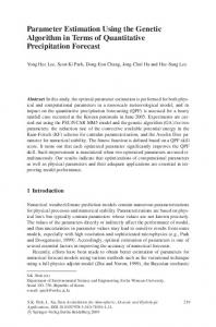
where ui are the inputs to the j t h unit (which may be inputs to the network, outputs from units in the previous layers, outputs from the unit itself, or outputs from units in succeeding layers). At each unit, the weight wj; and the bias bj are to be estimated. In this example, the GA is used to train the neural network model to perform bit rotations of input bit strings. For instance, if the input string is bl ,b 2 , b3, and the task is to rotate the string to the left by two places, then the desired output is b ~b l, , b 2 . A feedforward and a recurrent network are trained to perform this task. The structures of feedforward and recurrent network are shown in Figs. 3(a) and (b), respectively. A total of 64 randomly shuffled training pattems are generated in which the output patterns are contaminated by uniformly distributed

-:Feedforward Neural Net.

0.3

0.4

- - - :Recurrent Neural Net.

0.1 0.2

-*-._._

100

200

.... I00

400

500

1

600

Generation

Fig. 4. Estimation error convergence of feedforward and recurrent neural networks, Example 4.2.

noise between -0.1 and 0.1. For the feedforward and recurrent neural network, there are 24 parameters to be trained, whereas for the recurrent network, there are 19 parameters to be trained. Note that there are no hidden units in the recurrent network. The convergnce of the estimation error for both structures are shown in Fig. 4. 0 Example 4.34Modulated Sinusoidal Signals) In [25] and [26], it is shown that musical waveforms can be approximated based on a frequency modulation scheme. Let the music generation unit be given by m u ( t )= Asin (wct

+ Isin

(U&))

(4.4)

where A is a constant denoting the magnitude of the waveform,

w c is the carrier frequency, I is the modulation index, and w, is the modulating frequency. The musical waveform can be approximated by cascaded or parallel music generation units.

IEEE TRANSACTIONS ON SIGNAL PROCESSING, VOL. 42, NO. 4, APRIL 1994

934

- - - :Yl(t)

Refer to [25] and [26] for further details. In this example, the GA is applied to estimate the carrier, modulating frequencies, and modulation indices based on the modulated sinusoidal signals generated by the cascaded form I 03

and the parallel form y2(t)

= sin ( w 2 1 t

+

1 2 1 sin ( w 2 2 t ) )

+ sin ( W 2 3 t + 1 2 2 sin ( W 2 4 t ) ) -k n(t)

0

(4.6) -0.5

where n(.) is the measurement noise uniformly distributed between -0.25 and 0.25. The parameters are set to be

-1

.I.SL 0

*

100

>00

300

400

s00

600

100

800

900

I lo00

time X le-7 Fig. 5. Comparison of yl(t) and yl(t), Example 4.3.

Note that (4.5) and (4.6) can be considered to be nonlinear FIR filters so that the parameters can be estimated in the same way as in previous examples. The only difference is that all parameters to be estimated in this example are positive, which simplifies the coding of the chromosome. Let the sampling rate be lo7 samples/s for (4.5) and lo5 samples/s for (4.6). Accumulating the estimation errors for the 10oO samples (i.e., d = lOOO), the estimated parameters by the GA are

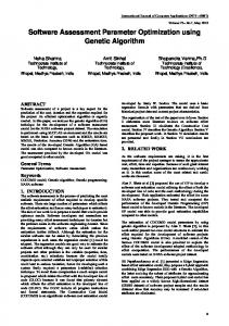
The modulated sinusoidal signals in (4.5) and (4.6) are compared in Figs. 5 and 6, respectively, with the signals $ l ( t ) and &(t), which are regenerated based on the estimated parameters. It is interesting to note that the parameter estimates are fundamentally different from their true values yet the regenerated signals based on these estimates match very well with the original signals. This demonstrates a fundamental lack of identifiability of the parameters in both (4.5) and (4.6). Equivalently, the system must be failing to satisfy some set of “persistance of excitation” conditions since the estimation errors converge towards zero even though the parameter values are not the same as used to generate the waveforms. V. CONCLUDING REMARKS

The genetic algorithm is a good tool for the optimization of nonlinear functions. When the GA is applied to parameter estimation problems, it is especially powerful for nonlinear IIR filters since it can be applied in situations where gradient methods fail and is not susceptible to problems with local

2 5I

-2.sL 0

1

*

100

I

200

300

400

100

600

700

800

900

lo00

lime X le-5 Fig. 6. Comparison of yz(t) and & ( t ) ,Example 4.3.

minima. The disadvantages of the GA stem from its computational complexity (when compared to a gradient approach) since it must process N different estimated parameter sets in each iteration. Thus, the GA should be seen primarily as a method for off-line identification, estimation, and optimization. Finally, it is not always obvious how to choose the user tunable parameters in an optimal fashion. REFERENCES [ l ] C. R. Johnson, Lectures on Adaptive Parameter Estimation. Englewood Cliffs, NJ: Prentice-Hall, 1988. [2] B.Widrow and S. D. Stems, Adaptive Signal Processing. Englewood Cliffs, NJ Prentice-Hall, 1985. [3] J. H. Holland Adaptation in Natural and Artijcial Systems. Ann Arbor, M I University of Michigan Press, 1975.

YAO AND SETHARES: NONLINEAR PARAMETER ESTIMATlON

D. E. Goldberg, Genetic Algorithms in Search. Optimization, and Machine Learning. New York: Addison-Wesley, 1989. K. De Jong, “A 10 year perspective,” in Proc. Int. Conf. Genetic Algorithms Their Applications, 1985, pp. 169-177. J. J. Grefenstette, “Optimization of control parameters for genetic algorithms,” IEEE Trans. Syst. Man. Cybern.. vol. SMC-16, no. 1, pp. 122-128, Jan.-Feb. 1986. L. Davis and M. Steenstrup, “Genetic Algorithms and simulated annealing,” in Genetic Algorithms and Simulated Annealing, L. Davis, Ed. London: Pitman, 1987, pp. 1-11. D. M. Etter and M. M. Masukawa, “A comparison of algorithms for adaptive estimation of the time delay between sampled signals,” in Proc. IEEE Int. CO$. ASSP, 1981, pp. 1253-1256, D. M. Etter, M. J. Hicks, and K. H. Cho, “Recursive adaptive filter design using an adaptive genetic algorithm,” in Proc. IEEE Int. Conf. ASSP, 1982, pp. 635-638. Y. Davidor, Genetic Algorithms and Robotics, A Heuristic Strategy for Optimization. Singapore: World Scientific, 1991. S . Matwin, T. Szapiro, and K. Haigh, “Genetic algorithms approach to a negotiation support system,” IEEE Trans. System Man Cybern., vol. 21, no. 1, pp. 102-114, Jan./Feb. 1991. R. Axelrod, “The evolution of strategies in the iterated prisoner’s dilemma,” in Genetic Algorithms and Simulated Annealing (L. David, Ed.). London: Pitman, 1987, pp. 32-41. K. De Jong, “Learning with the genetic algorithm: An overview,” Machine Learning, vol. 3, pp. 121-137, Oct. 1988. G. A. Vignaux and 2. Michalewicz, “A genetic algorithm for the linear transportation problem,” IEEE Trans. Syst. Man Cybern., vol. 21, pp. 445452, Mar./Apr. 1991. J. P. Cohoon, S . U. Hegde, W. N. Martin, and D. S. Richards, “Distributed genetic algorithm for the floorplan design problem,” IEEE Trans. Computer-Aided Des., vol. 10, pp. 483491, Apr. 1991. D. J. Montana and L. Davis, “Training feedfoward neural networks using genetic algorithms,” in Proc. Int. Joint Conf. Art$cial Intell.. (Detroit), 1989, p ~ 762-767. . H. Kitano, “Empirical studies on the speed of convergence of neural network training using genetic algorithms,” in Proc. Eighth Nut. Conf. Artificial Intell. (Boston), 1990, pp. 789-795. J. L. McClelland and D. E. Rumelhart, Parallel Distributed Processing. Cambridge, MA: MIT Press, 1986. F. J. F’ineda, “Generalization of backpropagation to recurrent and higherorder networks,” in Proc. IEEE CO$. Neural Inform. Processing Syst.. 1987, pp. 602-611. R. J. Williams and D. Zipser, “A learning algorithm for continually running fully recurrent neural networks,” Neural Comput., 1989, pp. 270-280. K. De Jong, “Using experience-based in game playing,” in Proc. 5th Int. Conf. Machine Learning (Ann Arbor, MI), 1988, pp. 284-290. H. Stark and J. W. Woods, Probability, Random Processes and Estimation Theory for Engineers.Englewood Cliffs, NJ: Prentice-Hall, 1986.

935

[23] K. S . Narendra and A. M. Annaswamy, Stable Adaptive Systems.Englewood Cliffs, N J Prentice-Hall, 1989. [24] J. M. Fitzpatrick and J. J. Grefenstette, “Genetic algorithms in noisy environments,” Machine karning, vol. 3, pp. 101-120, Oct. 1988. [25] J. Chowning, “The synthesis of complex audio spectra by means of frequency modulation,” J. Audio Eng. Soc., vol. 21, no. 7, pp. 526-534, 1973. [26] J. Chowning and D. Bristow, FM Theory andApplications, By Musicians for Musicians. Tokyo: Yamaha, 1986. [27] R. B. Ash, Basic Probability Theory. New York Wiley, 1970.

Leehter Yao (S’86-M’92) received the Ph.D. degree in electrical engineering from University of Wisconsin-Madison, in 1992. From 1988 to 1992, he was a research assistant in the Center for Health Systems Research and Analysis, University of Wisconsin. Since 1992, he has been with the Department of Electrical Engineering at the National Taipei Institute of Technology, Taiwan, R.O.C., where he is currently an associate professor. His research interests include adaptive systems in signal processing and automatid control, artificial intelligence, and pattem recognition.

William A. Sethares received the B.A. degree in mathematics from Brandeis University, Waltham, MA, and the M.S.and Ph.D. degrees in electrical engineering from Come11 University, Ithaca, NY. He has worked at the Raytheon Company as a Systems Engineer and is currently on the faculty of the Department of Electrical and Computer Engineering at the University of Wisconsin in Madison. His research interests include adaptive systems in signal processing, communications and control, electronic music, and other fashionabletopics. He especially enjoys writing brief biographical sketches.