Genetic Algorithms for Parallel Code Optimization Ender Özcan Dept. of Computer Engineering Yeditepe University Kayışdağı, İstanbul, Turkey Email:
[email protected] Abstract- Determining the optimum data distribution, degree of parallelism and the communication structure on Distributed Memory machines for a given algorithm is not a straightforward task. Assuming that a parallel algorithm consists of consecutive stages, a Genetic Algorithm is proposed to find the best number of processors and the best data distribution method to be used for each stage of the parallel algorithm. Steady state genetic algorithm is compared with transgenerational genetic algorithm using different crossover operators. Performance is evaluated in terms of the total execution time of the program including communication and computation times. A computation intensive, a communication intensive and a mixed implementation are utilized in the experiments. The performance of GA provides satisfactory results for these illustrative examples.
I. INTRODUCTION Data distribution and processor allocation are two important factors that affect the performance of programs written for distributed memory parallel architectures. Distribution of the data among the processors affects the communication time. On the other hand, the number of processors used at each step of the parallel code (degree of parallelism) affects both the computation time and the communication time. Different approaches have been used to solve the problem of optimizing data distribution in parallel programs [1]-[12]. These projects use a variety of optimization methods. There are also research works that present notation for communication-free distribution of arrays [13], [14]. The problem of finding optimal mappings of arrays for parallel computers is shown to be NP-complete [15]. As a discrete problem, even if a restricted set of data decomposition patterns is used, the nonlinear nature of the problem does not change, especially when combined with selecting the degrees of parallelism for each program stage and attempting to minimize the overall execution time. In this study, Genetic Algorithms (GA) is used to analyze the problem of determining the data distribution and the degree of parallelism for each stage of a parallel code in order to minimize the total execution time. II. PERFORMANCE CHARACTERIZATION OF PARALLEL ALGORITHMS A. Levels A serial algorithm may be composed of a sequence of stages (denoted as levels), where each stage is either a single loop or a group of nested loops (Figure 1(a)). An
Esin Onbaşıoğlu Dept. of Computer Engineering Yeditepe University Kayışdağı, İstanbul, Turkey Email:
[email protected] example program segment is given in Figure 6, where there are five levels. The entire sequence of levels may also be enclosed by an iterative loop (Figure 1(b)). A general case is given in Figure 1(c), where some consecutive loops are enclosed by iterative loops, which again with adjacent loops may be enclosed by other iterative loops and so on, like a tree structure. Here, to simplify the case, it is assumed that programs are in the form of Figure 1(a) and Figure 1(b), and programs that have structure as in Figure 1(c) are reduced to the form in Figure 1(b) by combining L2, L3, L4 as a single level.
[ L1 [ L2 [ L3 [ L4 [ L5
[ L1 [ L2 [ L3 [ L4 [ L5
[ L1 [ L2 [ L3 [ L4 [ L5
(a)
(b)
(c)
Figure 1. (a) sequence of levels, (b) sequence of levels enclosed by an iterative loop, (c) sequence of loops with a general structure
When the programs are parallelized, each level is assumed to have a different degree of parallelism that is, each level may be executed using a different number of processors. Levels requiring short computation may be parallelized on a few processors but those having long computations may require the use of many processors. Also, due to the distribution of the data among the processors, when the code is parallelized, communication may be required before the execution of each level. Although increasing the number of processors decreases the computation time of a level, it may cause extra communication between the levels. B. Performance Evaluation Performance of a serial algorithm can be expressed in terms of the problem size, but the performance of a parallel algorithm, in addition to the problem size, depends on the number of available processors, the distribution of the data among the processors, and the methods used for transferring data between processors. At some stage l of a parallel code, execution time (texec) can be expressed as the sum of the computation and communication times
l l l texec = tcomp + tcomm
Equation 1.,
l l where tcomp denotes the computation time, and tcomm
denotes the communication time at stage l. Computation time can be formulated as l l tcomp = tseq / pl
Equation 2.,
l where tseq is the predicted computation time of stage l of
the sequential algorithm on a single processor, and pl is the number of processors used in the parallel code for stage l. Communication time depends on the number of processors pl and the communication structure cl used for l the transfer of data at that stage. tcomm consists of two terms, a term that increases with the size of data to be transferred, represented by f1, and an overhead, represented by f2, l tcomm = f1 (cl , pl )dl + f 2 (cl , pl )
(a) Horizontal
(b) Replicated
(c) Rectangle
Figure 2. Possible decomposition patterns for a 1D array on 4 processors
(a) Horizontal
(b) Vertical
(c) Replicated
(d) Rectangle
Equation 3.,
where dl is the data size per processor. Note that both f1 and f2 are in the form (a pl + b), where a and b are constants that depend on the communication structure. The total execution time (T) of the program is the sum of the execution times of all stages in the program L
l T = ∑ texec
Equation 4.,
l =1
where L is the total number of stages (denoted as levels) in the code. In order to determine the execution time of a parallel program at compile-time, machine characterization and performance prediction method given in [16] is used. In this method, computation and communication characteristics of the machine are measured and formulated. In order to calculate the total execution time of a parallel program, its program parameters (i.e. computation time, data size) are substituted in the formulas. C. Data Decomposition and Alignment In most of the parallel algorithms, arrays of one or higher dimensions are used. In this study, arrays are assumed to be distributed to the processors in the form of blocks. Block decompositions of 1 and 2-dimensional arrays on four processors are illustrated in Figure 2 and Figure 3, respectively. It is assumed that all scalar values are replicated on all processors.
Figure 3. Possible decomposition patterns for a 2D array on 4 processors
Arrays are distributed to the processors according to one of the decomposition patterns, presented in Figure 2 and Figure 3. Due to the computational requirements, arrays existing at a level, may be distributed to processors using the same or different decomposition patterns. Considering all the arrangements of decomposition patterns for all the arrays at a level, some of them may not be feasible. Feasible arrangements of decomposition patterns of arrays at a level are referred as alignment. As an example, possible alignments for the third level of the code in Figure 7 are demonstrated in Table I. The arrangement, (Horizontal, Vertical, Horizontal), for arrays c, I and b is not a feasible arrangement, as it can not satisfy the computational requirements. Hence, it is not accepted as an alignment. TABLE I. ALLIGNMENTS FOR THE THIRD LEVEL OF THE CODE IN FIGURE 7
Array c I b
Alignment 1 Horizontal Horizontal Horizontal
Alignment 2 Vertical Vertical Vertical
Alignment 3 Rectangular Rectangular Rectangular
D. Communication Structures In distributed memory architectures using messagepassing, generally, data is transferred among the processors in a structured way. Different communication structures have been defined for data exchange between processors [17], [18]. In this study, multiphase (MU), shift (SH), broadcast (BR), scatter (SC) and gather (GA) structures have been utilized (Figure 4).
references to the same arrays in the upper and lower levels of the code. Then, a common feasible communication structure is selected. In this work, instead of selecting the communication structure randomly, the one that produces the minimum transfer time is selected. In order to minimize the program execution time, the best number of processors for each level of the code and the best alignment for the arrays that are referred to at each level of the code must be determined. A parallel code might consist of many levels. Furthermore, for each level there might be different possibilities for alignment, degree of parallelism and communication structure. For this reason, the problem of finding the optimal parallel code configuration becomes highly complex. III. GENETIC ALGORITHMS FOR PARALLEL CODE OPTIMIZATION
(a) Multiphase
(b) Broadcast
(c) Scatter
(d) Gather
(e) Shift Figure 4. Five types of communication structures used in the study
Performance of the communication structures can be characterized in terms of f1 and f2, as shown in Table II. For all structures, f1 and f2 depend on the number of processors, except for SH, where f1 and f2 are constant. The machine parameters M, N, R and Q are measured running benchmarks on the parallel machine, as explained in [16]. The hardware platform used in this study consists of 16 Pentium 4, 2GHz processors connected by 100Mbit/s interconnection network. TABLE II. MACHINE PARAMETERS FOR THE COMMUNICATION STRUCTURES
c MU BR SC GA SH
f1 (cl , pl )
M1 M3 M4 M5 N2
pl pl pl pl
+ N1 + N3 + N4 + N5
f 2 (cl , pl )
R1 R3 R4 R5 Q2
pl pl pl pl
+ Q1 + Q3 + Q4 + Q5
Once the data distribution and the number of processors at each level are determined, communication structures to be inserted between levels can be selected. For each level, feasible communication structures, that are valid for all arrays at that level, are identified considering the
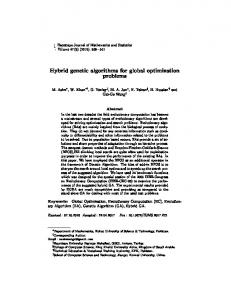
Genetic Algorithms have been used for solving many difficult problems [19] that were introduced by J. Holland in 1975 [20]. Given a parallel code, consisting of L levels and a distributed memory parallel machine with P processors, parallel code optimization (PCO) can be stated as finding the best mapping of P processors and D alignments of data decomposition patterns at each level, reducing the total expected execution time of the algorithm. The search space ranges up to (PD)L, assuming the best communication structure for the level. Although not considered in here, the size of a level and selecting the levels to combine may also be used as other optimization parameters. Machine parameters are obtained by Benchmarking as explained in [16] and fed into the GA Solver for execution time optimization as shown in Figure 5. The Alignment Parser parses the given sequential code to be parallelized, in a C like language. It determines all possible array alignments in the code and generates the related data decomposition patterns at all levels, handing them over to the GA solver. Finally, GA solver produces the best assignment of alignments and number of processors at each level. Sequential Code
Alignment Parser
Bechmarking
GA Solver
Figure 5. Flowchart showing how parallel code optimization problem is solved by GA
A. GA Components Each individual is a list of alleles, where each locus represents a level in the given code. Alleles consist of two parts: number of processors to be used at a level and the data alignment. Figure 6 demonstrates an example individual, having 5 levels.
1 4
2 2
4
3 1
4
4 5
1
5 1
1
1
4 processors and 5th alignment should be used at level 3 Figure 6. An example individual representing a candidate solution for a PCO problem with 5 levels
Two types of Genetic Algorithms are implemented as a solver: steady state genetic algorithms (SSGA) and transgenerational genetic algorithms (TGGA). Population size is chosen to be proportional to the length of an individual. Fitness function indicates the total execution time as shown in Equation 4. The best communication structure is chosen at each level among all possibilities. This step can be considered as a hill climbing step. This process can be applied, since the contribution of the communication structure to the total execution time at each level is independent. SSGA and TGGA both utilize linear ranking strategy for selecting parents and elitist replacement strategies. In SSGA, two worst individuals in the population are deleted and both offspring are injected in their places. In TGGA, the best of the offspring combined with the previous population forms the next generation. SSGA visits two new states at each generation, while the number of states that TGGA visits is two times the individual length, determining the number of evaluations. Different crossover operators are tested: traditional one point crossover (1PTX), two-point crossover (2PTX) and uniform crossover (UX). Traditional mutation is used, randomly perturbing an allele, assigning a random value to the number of processors and the decomposition pattern. Runs are terminated, whenever the expected fitness is reached or the maximum number of generations is exceeded. IV. EXPERIMENTAL DATA Experiments are performed using three data sets produced from two different algorithms. A. Hessenberg Reduction In the first and second data sets, the parallel algorithm in [21] for reducing matrices to Hessenberg form is used.
One iteration of the Hessenberg reduction is represented as follows:
A = (I – V Z VT)T A (I – V Z VT), where A, Z, V are NxN matrices. Its parallel implementation has 5 levels as shown in Figure 7. Levels 1, 2, 4 and 5 perform matrix multiplication operation where the execution time increases with N3, and level 3 consists of a subtraction operation where the execution time increases with N2. for (i=0; i