Appendix Table S3: Promoter and terminator part characterization in Erlenmeyer flasks. 16. Appendix Table S4: Sensor and gate response function parameters ...
Appendix for: Genetic circuit characterization and debugging using RNA-seq
Thomas E. Gorochowski, Amin Espah Borujeni, Yongjin Park, Alec A.K. Nielsen, Jing Zhang, Bryan S. Der, D. Benjamin Gordon and Christopher A. Voigt Appendix Text Appendix Text S1: Transcription profile correction method Appendix Text S2: Measurement of ribozyme performance from RNA-seq data
2 2 5
Appendix Figures Appendix Figure S1: Appendix Figure S2: Appendix Figure S3: Appendix Figure S4: Appendix Figure S5: Appendix Figure S6: Appendix Figure S7: Appendix Figure S8:
6 6 7 8 9 10 11 12 13
Appendix Tables Appendix Table S1: Appendix Table S2: Appendix Table S3: Appendix Table S4:
Distribution of fragment length versus circuit position Transcription profile replicates, measured on different days Sequenced fragment length distributions Ribozyme transcription profiles for cells grown in culture tubes Antisense transcription across the circuit Transcription profiles for parts when cells are grown in Erlenmeyer flasks Sensor and gate response functions when cells are grown in Erlenmeyer flasks Circuit plasmid
14 14 15
Ribozyme part characterization in culture tubes Top 25 down and up regulated genes for states where four circuit genes are expressed Promoter and terminator part characterization in Erlenmeyer flasks Sensor and gate response function parameters in Erlenmeyer flasks
16 17
Appendix Table S5: Genetic part sequences
18
Appendix References
21
1
Appendix Text S1: Transcription profile correction method RNA-seq measurements generate millions of fragments that are computationally mapped to sequences for the genetic circuit and host genome. The transcription profile is created via this process. This is adequate for many applications in systems biology where gene expression can be inferred by averaging the profile across the length of a gene. However, there is a bias that occurs during the mapping process that causes a gradual decline at the 5’- and 3’- ends of each transcription unit. By definition, promoters and terminators occur at these boundaries. While it is easy to qualitatively detect that these parts exist (and this is the basis for algorithms to detect promoters/terminators in the genome), the decline complicates the quantitative calculation of their strength, which is important in synthetic biology. Therefore, we developed a method to correct for these edge effects that utilizes the empirical fragment length distribution from the RNA-seq experiment. The distribution is used to create a single correction factor that is applied to all of the 5’- and 3’- ends of the transcripts in the circuit. After this process, the equations to calculate part strength are applied. Note that this correction factor is only applied to the transcripts corresponding to the gates in the circuit; it is not applied to internal promoters, antisense transcription, or genomic expression (in these cases, it is not necessary to calculate part strength). Below, when we refer to the transcripts in the circuit, this only encompasses transcripts originating from transcription start sites within the input/output promoters in the gates. Each RNA-seq experiment has a unique fragment length distribution, which depends on many growth-related and growth-unrelated processes (Klumpp et al, 2009; Roberts et al, 2011). Inside cells, the length and abundance of mRNA transcripts at steady-state is controlled by a balance between several processes such as transcriptional bursting, elongation and termination, RNA polymerase fall-off, and mRNA degradation. Outside the cells, after total RNA extraction, mRNA transcripts undergo several post-processing modifications such as fragmentation, reverse transcription, PCR amplification, and DNA selection before being sequenced using high-throughput sequencing systems. Importantly, these post-processing steps will define the final shape of fragment length distribution. Two main contributing factors to this shape are the positional biases introduced during the post-processing and sequencing events, and the loss of RNA fragments (mostly occurring during the DNA selection step). The profile bias at the ends of a transcript occurs because a fragment is more likely to map at the center of the transcript and less likely at the ends. Differences in the fragment length distribution impact the shape of the profile. Long fragments have the effect of exaggerating the bias (it extends deeper into the transcript from each end) as compared to short ones. Here, we sought to create a simple method that calculates a correction factor based on the fragment length distribution and apply it to all the transcription
2
units in the circuit. Alternatively, the fragment length distribution for each transcription unit, as opposed to the experiment as a whole, could be calculated and applied. However, we found that this was unnecessary because the transcription units are all about the same size due to the fact that they encode single TetRfamily repressors. The first step in our correction method is to generate a distribution of all the fragment lengths mapped across the circuit and the genome (Appendix Figure S3). Because we use paired-end sequencing, the position of the start and end of each fragment is known, enabling the length to be directly calculated. We then consider a hypothetical 2000 nt transcription unit to generate a calculated profile T(x) that captures the expected curvature across a transcript within the transcription profile. This is generated by stochastically selecting a number of lengths (100,000) from the fragment length distribution and randomly mapping fragments of these lengths to the hypothetical transcription unit. T(x) is then produced by counting the number of mapped fragments per nucleotide (Box 1). In order to generate a general correction factor profile C(x), the hypothetical profile T(x) is normalized with respect to its maximum. We found that the impact of the correction is negligible after ~400 nt , in other words C(x) ⟶ 1, so only the first 500 nt of C(x) are used. This correction factor is only based on the length of the fragments and does not consider their sequence. Thus, the effect is identical at the 5’- and 3’- ends of the transcript and the same correction factor can be applied to both ends. Next, the transcription profile P(x) is generated for transcription units across the circuit. It is not applied to regions where part strengths do not have to be calculated, such as genomically-encoded genes. First, fragments from the RNA-seq data mapping within the boundaries of a single transcription unit are identified. These are used to generate P(x) by counting the number of fragments covering each nucleotide x. To correct the curvature present at the ends of each transcription unit (Box 1), we divide the first and last 500 nt of each transcription unit in P(x) by C(xn), where xn is the distance in nucleotides to the nearest end of the transcription unit. Finally, all remaining fragments from the RNA-seq data (i.e., those mapping outside the previously considered transcription units or spanning transcription unit boundaries) are combined with Pc(x) to produce the final transcription profile. To enable comparison of absolute changes in the profiles between samples, M(x) is further normalized by F = m/106, where m is the effective library size calculated for each RNA-seq experiment using a trimmed mean of M-values (TMM) approach (Robinson & Oshlack, 2010) (Dataset EV1). This method accurately corrects the curvature at the two ends of all transcription units in the circuit. However, issues were observed for the LitR and BM3R1 genes for state –/–/+ when grown in culture tubes (specifically for biological replicate 1). For these genes, the 3’-end of the corrected profiles unexpectedly
3
rises (Figure 2D). This was due to a large number of fragments having their 3’-end mapping to the 3’-end of these transcription units (Appendix Figure S1). This feature was only present for one of the biological replicates and not seen across the other samples (Appendix Figure S2).
4
Appendix Text S2: Measurement of ribozyme performance from RNA-seq data Ribozyme insulators were present at all promoter-RBS junctions to cleave variable 5’ sequences generated by differing upstream promoters. Inspection of the transcription profiles revealed that for both single and pairs of promoters, increases in the profiles occurred not at the transcription start site (xTSS) of each promoter, but instead at the cut-site of the nearest downstream ribozyme insulator (Appendix Figure S5B). The reason for this could be traced to the preparation of the sequencing libraries. Because ribozymes are located near the start of the 5’-UTR of each transcript, after cleavage, a short ~80 bp fragment is generated in addition to a longer fragment containing the downstream gene. Short-cleaved fragments were undetected during sequencing because reverse transcribed cDNA fragments of less than 100 bp were filtered during library preparation (Appendix Figure S4). This resulted in the transcription profiles lacking information for the beginning of these transcripts. A byproduct of this filtering was that it allowed us to characterize ribozyme cleavage. Because short cleaved RNA fragments were filtered and uncleaved fragments were captured during sequencing, by comparing the transcription profile directly after the cut-site (capturing both cleaved and uncleaved fragments) to the transcription profile at the beginning of the ribozyme (only capturing uncleaved fragments), the fraction of cleaved fragments pc can be calculated as 𝑝" =
() *+ $(&)/ ,-() *. () 1+ $(&)/ ,-() 1.
(0 1+ ,-(0 1. $ (0 1+ $ ,-(0 1.
& &
.
(S1)
Here, xC is the position of the ribozyme’s cut-site, x0 is the start position of the first upstream promoter, and n is the window length (Appendix Figure S5A). Transcripts originating from upstream of the ribozyme’s associated promoter (Appendix Figure S5A) are subtracted because cleavage of these will generate fragments with a length that is too large to be filtered during library preparation and would thus confound the calculation.
5
0.008
Probability
A
B
5’-end Alignment
0.004
-/-/-
3’-end Alignment Counts
400
400
200
200
0
0
400
400
200
200
0
0
400
400
102
200
200
101
0
0
400
400
200
200
0
0
400
400
200
200
0
0
400
400
102
200
200
101
0
0
400
400
102
200
200
101
0
0
400
400
200
200
0
0
0 0
200
400
600
+/-/-
Fragment Length (bp) Uniform Mapping
-/+/Fragment Length (bp)
Mapped Profile
100,000 Fragments
105 104 103 10
2
0
200
400
600
800
Position (bp)
+/+/-
-/-/+
Fragment Length (bp)
+/-/+
5’-end Alignment 600
600
400
102
400
200 0 0
-/+/+
3’-end Alignment Counts
10
200
200 400 600 800
0 0
1
+/+/+
101
102 101
103 101
103 101
102 101
100 200 400 600 800
LitR LitR Appendix Figure S1: Distribution of fragment length versus circuit position. (A) A hypothetical fragment length distribution was generated by randomly selecting 100,000 values from a gamma probability density function that mimics the experimental fragment length distributions (shape = 12 and scale = 23). Fragments were uniformly mapped to random positions within an 800 nt hypothetical transcription unit, and a transcription profile generated by counting the number of fragments spanning each nucleotide position. Heat-maps show how fragments of different lengths are distributed across the transcription unit. At all positions, the number of mapped fragments with specific lengths follows the original fragment length distribution. The right-angled trapezoid shape of the heat-maps is the result of fragments having to map within the boundaries of the transcription unit. (B) Distribution of length versus position are shown for fragments mapped exclusively within the borders of LitR. Data shown for experiments performed in culture tubes. LitR is actively transcribed for six induction states (–/+/–, +/+/–, –/–/+, +/–/+, –/+/+ and +/+/+). These states show a near uniform mapping and no positional bias, apart from state –/–/+. For this state, a significant number of fragments map to the 3’-end of LitR, which explains the rise in the corrected transcription profiles at this point (Figure 2D). Position (bp)
Position (bp)
6
105 2 −/−/− 10 2 -10 105 2 +/−/− 10 2 -10
Transcription Profile, M(x) (au)
−/+/−
105 102 -102
+/+/−
105 102 -102
105 2 −/−/+ 10 2 -10
+/−/+
−/+/+
105 102 -102 105 102 -102
105 2 +/+/+ 10 2 -10
AmtR
LitR
BM3R1
SrpR
PhlF
yfp
AraC
Appendix Figure S2: Transcription profile replicates, measured on different days. Separate lines are shown for each of the three biological replicates. Transcription profiles for the sense strand are colored grey and red for the antisense strand.
7
Lac
0.006
+/-/-
-/-/+ -/+/-
+/-/+ +/+/-
+/-/+
100 300 500 -/+/+ Length (bp)
100 300 500 +/+/+ Length (bp)
0.000 300 300 500 500100 300 500 100 300 500100 100 Length (bp) (bp) Length (bp) Length (bp) Length
100 300 500 Length (bp)
100 300 500 Length (bp)
Density
-/-/-
A
Replicate 1 0.006 -/+/-
+/-/-
0.002
0.002
0.002 100 300 500 Length (bp)
100 300 500 Length (bp)
0.004 0.002 0.000
0.006 -/+/+
+/-/+
Density
Density
-/-/+
0.004
0.000
0.004
0.000
0.000 0.006
0.006 +/-/-
-/-/-+/+/Density
-/-/-
0.002
C0.000 Density
Density
0.006 0.004
0.004
-/-/++/+/+
0.004 0.002
Replicate 2 Density
0.006
-/-/-
+/-/-
-/+/-
+/+/-
-/-/+
+/-/+
-/+/+
+/+/+
100 300 500 Length (bp)
100 300 500 Length (bp)
100 300 500 Length (bp)
100 300 500 Length (bp)
0.004 0.002 0.000
Density
0.006 0.004 0.002 0.000
Replicate 3 Density
0.006
-/-/-
+/-/-
-/+/-
+/+/-
-/-/+
+/-/+
-/+/+
+/+/+
100 300 500 Length (bp)
100 300 500 Length (bp)
100 300 500 Length (bp)
100 300 500 Length (bp)
-/-/-
+/-/-
-/+/-
+/+/-
-/-/+
+/-/+
-/+/+
+/+/+
100 300 500 Length (bp)
100 300 500 Length (bp)
100 300 500 Length (bp)
100 300 500 Length (bp)
0.004 0.002 0.000
Density
0.006 0.004 0.002 0.000
B Density
0.006 0.004 0.002 0.000
Density
0.006 0.004 0.002 0.000
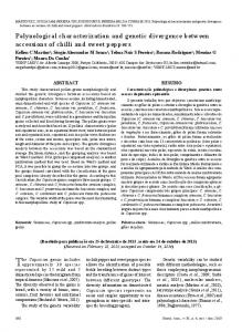
Appendix Figure S3: Sequenced fragment length distributions. (A) Circuit grown in culture tubes (data shown for three biological replicates) and (B) Erlenmeyer flasks for all combinations of inputs. (C) Modified version of the circuit grown in culture tubes. Each distribution shows the combination of inputs (IPTG/aTc/Ara) in the top right corner. The shaded regions (0 to 78 bp) represent the length of the longest 5’UTR fragment produced after ribozyme cleavage.
8
100 30 Lengt
A
Transcription Profile, M(x)
01 Forward Parts
δJ
01 Forward Parts 02 Reverse Parts
x0 −10
xTSS x0
Transcription Profile M(x) (au)
B
106 10
BydvJ
5
106 10
PlmJ
106
5
10
xC −10 xC xC +10 x2
x1 Postion, x (bp)
SarJ
RiboJ10
02 Reverse 106 Parts 106 03 Custom Properties
5
10
5
10
RiboJ53
5
106 10
104
104
104
104
104
104
103
103
103
103
103
103
102
102
102
102
102
102
101
101
101
101
101
101
0 0
50 100 150 200 250
Position (bp)
0 0
120 240 360 480
Position (bp)
0 0
0 0
120 240 360
Position (bp)
50 100 150 200
Position (bp)
0 0
50 100 150 200 250
Position (bp)
03 Custom Properties
RiboJ
5
0 0
50
100
150
Position (bp)
Appendix Figure S4: Ribozyme transcription profiles for cells grown in culture tubes. (A) Method for characterizing ribozyme cleavage (Appendix Text S2). The fraction of cleaved fragments by the ribozyme is calculated as 𝑝" =
4) 56 &74) 58 𝑀(𝑖)
−
associated promoter is given by 𝛿𝐽
40 /6 &740 /8 𝑀 𝑖 < 4) 56 = &74) 58 𝑀 6
4) /6 &74) /8 𝑀(𝑖)
𝑖 −
−
40 /6 &740 /8 𝑀
40 /6 &740 /8 𝑀
𝑖 and the activity of the
𝑖 with n = 10 bp. (B) Transcription
profiles for the ribozyme parts. Lines show the transcription profile for each of the 8 input states. Shaded regions denote the location of the ribozyme and dashed line shows the cleavage site. Data shown for biological replicate 1.
9
−/−/−
+/−/−
Transcription Profile, M(x) (au)
−/+/−
+/+/−
−/−/+
+/−/+
−/+/+
+/+/+
A
B
105 102
105 102
102 105 105 102 102 105 105 102 102 105 105 102 102 105 105 102 102 105 105 102 102 105 105 102 102 105 105 102 102 105 AmtR
▴
▴
▴
▴
▴
▴
▴
▴
▴
▴
▴
▴
▴
▴
▴
▴
LitR
102 105 105 102 102 105 105 102 102 105 105 102 102 105 105 102 102 105 105 102 102 105 105 102 102 105 105 102 102 105 BM3R1
SrpR
PhlF
AmtR
yfp
▴
▴
▴
▴
▴
▴
▴
▴
▴
▴
▴
▴
▴
▴
▴
▴
LitR
BM3R1
SrpR
PhlF
yfp
Appendix Figure S5: Antisense transcription across the circuit. Data for all input states shown for cells grown under (A) culture tube (data shown for biological replicate 1) and (B) Erlenmeyer flask conditions. Transcription profiles are shown for both sense (gray) and antisense (red) strands. Light gray shaded regions denote the location of terminator parts. Triangles mark the antisense promoter present within PBAD.
10
Transcription Profile M(x) (au)
01 Forward Parts
106
PTac PTet1
5
106
PBAD1 PTet2
106
PBAD2
106
PBM3R1 PAmtR
106
PSrpR PLitR
01 Forward Parts 10 02 Reverse Parts 104
105
105
105
105
105
104
104
104
104
104
103
103
103
103
103
103
102
102
102
102
102
102
101
101
101
101
101
101
0 0
106
60 120 180 240
L3S2P55
106
Transcription Profile M(x) (au)
02 Reverse Parts 5 10 03 Custom Properties 01 Forward Parts 104
10
150
300
450
L3S2P24
0 0
106
5
10
150
0 450 0
300
L3S2P11
106
5
10
60
120 180
ECK120029600
5
0 0
106 10
0 0
60 120 180 240
ECK120033737
5
106 10
104
104
104
104
103
103
103
103
103
103
102
102
102
102
102
102
101
101
101
101
101
101
0 0
02 Reverse Parts 10
30
60
90
BydvJ
5
0 0
30
90
PlmJ
106 10
60
5
0 0 106 10
30
60
0 0
90
SarJ
106
5
10
30 60 90 120
RiboJ10
5
0 0 106 10
30
60
0 0
90
RiboJ53
5
106 10
104
104
104
104
104
103
103
103
103
103
103
102
102
102
102
102
102
101
101
101
101
101
101
0 50 100 150 200 250 0
120 240 360 480
Position, x (bp)
Position, x (bp)
0 0
120 240 360
Position, x (bp)
03 Custom Properties
0 0
50 100 150 200
Position, x (bp)
0 0
50 100 150 200 250
Position, x (bp)
120
L3S2P21
30
60
90
RiboJ
5
104
0 0
60
5
104
03 Custom Properties 106 Transcription Profile M(x) (au)
0 0
PPhlF
106
0 0
50
100
150
Position, x (bp)
Appendix Figure S6: Transcription profiles for parts when cells are grown in Erlenmeyer flasks. Lines show the transcription profile for each of the 8 input states. Shaded regions denote the location of the relevant part. For promoters, the lines are black when the promoter is expected to be on and red when it is expected to be off. The ribozyme cleavage site is denoted by a dashed line.
11
A Output, δJ (au/s)
PTac
PTet1
PTet2
PBAD2
103
103
103
103
102
102
102
102
102
1
1
1
1
101 100
10
10
10
10
100
100
100
100
0
0
0
0
- IPTG +
B
-
PAmtR Output, δJ (au/s)
PBAD1
103
aTc
+
-
PLitR
Ara
+
0
-
PBM3R1
aTc
+
-
PSrpR
103
103
103
103
102
102
102
102
102
1
1
1
1
101
100
100
10
100 0 0
10
100 100 101 102 103
Input, J (au/s)
0 0
10
100 100 101 102 103
Input, J (au/s)
0 0
100 101 102 103
Input, J (au/s)
0 0
100 101 102 103
Input, J (au/s)
+
PPhlF
103
10
Ara
0 0
100 101 102 103
Input, J (au/s)
Appendix Figure S7: Sensor and gate response functions when cells are grown in Erlenmeyer flasks. (A) The response of the output promoters of the sensors are shown in the presence and absence of each inducer. The dashed lines show the sensor outputs measured in isolation (Nielsen et al, 2016). The boxes show the median (grey line) and range of promoter activities measured for the four states where it is off (dJoff) and four where it is on (dJon). (B) Solid colored lines show the response functions of the gates obtained by fitting the promoter activities to the RNA-seq data (circles denote the measured values for the 8 input states). The dashed lines show the output of the gate measured in isolation (Nielsen et al, 2016). The fit parameters for the response functions are provided in Appendix Table S4.
12
BydvJ
L3S2P55
PlmJ
AmtR PTac PTet
L3S2P24 SarJ
LitR PBAD PTet
L3S2P11
RiboJ10 ECK120029600 RiboJ53 ECK120033737 RiboJ
BM3R1 PBAD
PhlF
SrpR PBM3R1 PAmtR
PSrpR PLitR
L3S2P21
YFP PPhlF
pAN0x58v50 J23105
KanR
p15A
TetR
LacI
AraC
PLacI
Appendix Figure S8: Circuit plasmid. Parts names are shown for all genes, promoters, terminators, and ribozymes. Part sequences are provided in Appendix Table S5.
13
Appendix Table S1: Ribozyme part characterization in culture tubes. Ribozyme
Genetic Context a,b
b,c
Isolation
Circuit
BydvJ PlmJ SarJ
0.98 0.97 0.99
0.99 ± 0.0 0.99 ± 0.0 0.99 ± 0.0
RiboJ10 RiboJ53 RiboJ
0.98 0.99 0.97
0.99 ± 0.0 0.98 ± 0.0 0.99 ± 0.04
a. Measurements from Nielsen et al (2016). b. Ribozyme cleavage values given as a fraction of the total cleaved to 2 s.f. c. Average and standard deviation calculated from three replicates performed on different days for states where the transcript is expressed.
14
Appendix Table S2: Top 25 down and up regulated genes for states where four circuit genes are expressed Gene
log2 foldchange
yncA flu ygiP yqeC ydcZ napF ndk nikA dmsA tpx rraA ansB yjjI yedE
-5.0 -3.6 -3.6 -3.8 -3.3 -4.2 -2.4 -3.4 -3.8 -2.0 -2.8 -2.7 -3.8 -3.3
hypB yccM napA yhbU yjjW yhjX sodB csiE pepT yiaU yncA nrdE nrdF nrdI yjjZ rcsA fhuE yedA sufD nrdH sufS yjbE add xylF fhuF araJ eptA acrD yagG asnB yedV cirA sufC ydeH gmd sufE
-3.1 -3.0 -3.6 -3.5 -3.2 -2.5 -1.6 -2.4 -2.4 -2.4 -5.0 3.6 3.7 4.1 4.3 5.8 3.0 3.4 2.0 3.1 2.0 5.9 1.8 4.8 1.5 4.6 2.5 2.1 1.6 1.7 2.2 2.0 2.0 2.1 4.9 2.1
Description
Related pathways and role
50S ribosomal protein L36 paralog Self-recognizing antigen 43 (Ag43) autotransporter DNA-binding transcriptional activator TtdR Uncharacterized protein Uncharacterized protein Ferredoxin-type protein Nucleoside diphosphate kinase Ni(2+) ABC transporter periplasmic binding protein Dimethyl sulfoxide reductase subunit A Lipid hydroperoxide peroxidase Ribonuclease E inhibitor protein A Asparaginase II Uncharacterized protein Uncharacterized protein GTP hydrolase (nickel liganding into hydrogenases)
Protein acetylation Integral component of membrane – – – Response to oxidative stress Nucleotide biosynthesis Nickel cation transport Anaerobic respiration Cellular response to oxidative stress RNA metabolism Amino acid metabolism – – Protein maturation and complex assembly
Uncharacterized protein Periplasmic nitrate reductase subunit Uncharacterized protein Uncharacterized protein Uncharacterized protein Superoxide dismutase (Fe) Stationary phase inducible protein Peptidase T Uncharacterized protein L-amino acid N-acyltransferase Ribonucleoside-diphosphate reductase 2, α subunit dimer Ribonucleoside-diphosphate reductase 2, β subunit dimer Flavodoxin Uncharacterized protein DNA-binding transcriptional activator Ferric coprogen/ferric rhodotorulic acid transporter Uncharacterized protein Fe-S cluster scaffold complex subunit Glutaredoxin-like protein L-cysteine desulfurase Uncharacterized protein Adenosine deaminase Xylose ABC transporter periplasmic binding protein Hydroxamate siderophore iron reductase Uncharacterized protein Phosphoethanolamine transferase Multidrug efflux pump RND permease Uncharacterized protein Asparagine synthetase B Sensory histidine kinase Ferric dihyroxybenzoylserine outer membrane transporter Fe-S cluster scaffold complex subunit Diguanylate cyclase GDP-mannose 4,6-dehydratase Sulfur acceptor for SufS cysteine desulfurase
– Anaerobic respiration – – – Oxidation-reduction process Transcription regulation Proteolysis – Protein acetylation DNA replication DNA replication Protein modification – Transcriptional regulation of colonic acid Iron ion homeostasis – Response to oxidative stress Cell redox homeostasis Sulphur compound metabolism – DNA damage response and purine salvaging Carbohydrate transport Iron assimilation – Response to antibiotics and lipid metabolism Response to drug and drug transport – Amino acid biosynthesis DNA damage response Iron assimilation Iron-sulfur cluster assembly Regulation of cell motility Colanic acid biosynthesis Response to oxidative stress
15
Appendix Table S3: Promoter and terminator part characterization in Erlenmeyer flasks. Promoter(s) PTac-PTet1 PBAD1-PTet2 PBAD2
a
Strength 6, 9 213, 115 27
PBM3R1-PAmtR PSrpR-PLitR PPhlF
7, 45 12, 26 533
Terminator
Strength
L3S2P55 L3S2P24 L3S2P11 ECK120029600 ECK120033737 L3S2P21
b
25 179 70 260 793 98
a. Average promoter strengths are shown in au/s for each promoter when on. For double promoters, strengths are calculated separately when only one of the promoters is predicted to be on. b. Median terminator strengths are calculated for states where the upstream gene is predicted to be in an on state.
16
Appendix Table S4: Sensor and gate response function parameters in Erlenmeyer flasks. a
Sensor
dJoff
dJon
PTac PTet1 PTet2 PBAD1 PBAD2
0.0 0.0 0.0 0.0 0.0
10 13 167 265 27
b
dJoutmin
dJoutmax
K
n
0.6 1.4 0.0 0.4 0.9
66 31 7 23 523
1.1 1.6 3.3 2.4 11.6
2.3 1.3 4.0 2.3 4.0
Gate PAmtR PLitR PBM3R1 PSrpR PPhlF a. b.
In units of au/s. min max Parameters dJout , dJout and K are in units au/s.
17
Appendix Table S5: Genetic part sequences
Part Name AmtR
Type Gene
DNA Sequence
LitR
Gene
ATGGATACCATTCAGAAACGTCCGCGTACCCGTCTGAGTCCGGAAAAACGTAAAGAACAGCTGCTG GATATTGCCATTGAAGTTTTTAGCCAGCGTGGTATTGGTCGTGGTGGTCATGCAGATATTGCAGAA ATTGCACAGGTTAGCGTTGCAACCGTGTTTAACTATTTTCCGACCCGTGAAGATCTGGTTGATGAT GTTCTGAACAAAGTGGAAAACGAGTTTCACCAGTTCATCAATAACAGCATTAGCCTGGATCTGGAT GTTCGTAGCAATCTGAATACCCTGCTGCTGAACATTATTGATAGCGTTCAGACCGGCAACAAATGG ATTAAAGTTTGGTTTGAATGGTCAACCAGCACCCGTGATGAAGTTTGGCCTCTGTTTCTGAGCACC CATAGCAATACCAATCAGGTGATCAAAACCATGTTTGAAGAGGGTATTGAACGCAATGAAGTGTGC AATGATCATACACCGGAAAATCTGACCAAAATGCTGCATGGTATTTGCTATAGCGTGTTTATTCAG GCCAATCGTAATAGCAGCAGCGAAGAAATGGAAGAAACCGCAAATTGCTTTCTGAATATGCTGTGC ATCTACAAATAA
BM3R1
Gene
ATGGAAAGCACCCCGACCAAACAGAAAGCAATTTTTAGCGCAAGCCTGCTGCTGTTTGCAGAACGT GGTTTTGATGCAACCACCATGCCGATGATTGCAGAAAATGCAAAAGTTGGTGCAGGCACCATTTAT CGCTATTTCAAAAACAAAGAAAGCCTGGTGAACGAACTGTTTCAGCAGCATGTTAATGAATTTCTG CAGTGTATTGAAAGCGGTCTGGCAAATGAACGTGATGGTTATCGTGATGGCTTTCATCACATTTTT GAAGGTATGGTGACCTTTACCAAAAATCATCCGCGTGCACTGGGTTTTATCAAAACCCATAGCCAG GGCACCTTTCTGACCGAAGAAAGCCGTCTGGCATATCAGAAACTGGTTGAATTTGTGTGCACCTTT TTTCGTGAAGGTCAGAAACAGGGTGTGATTCGTAATCTGCCGGAAAATGCACTGATTGCAATTCTG TTTGGCAGCTTTATGGAAGTGTATGAAATGATCGAGAACGATTATCTGAGCCTGACCGATGAACTG CTGACCGGTGTTGAAGAAAGCCTGTGGGCAGCACTGAGCCGTCAGAGCTAA
SrpR
Gene
ATGGCACGTAAAACCGCAGCAGAAGCAGAAGAAACCCGTCAGCGTATTATTGATGCAGCACTGGAA GTTTTTGTTGCACAGGGTGTTAGTGATGCAACCCTGGATCAGATTGCACGTAAAGCCGGTGTTACC CGTGGTGCAGTTTATTGGCATTTTAATGGTAAACTGGAAGTTCTGCAGGCAGTTCTGGCAAGCCGT CAGCATCCGCTGGAACTGGATTTTACACCGGATCTGGGTATTGAACGTAGCTGGGAAGCAGTTGTT GTTGCAATGCTGGATGCAGTTCATAGTCCGCAGAGCAAACAGTTTAGCGAAATTCTGATTTATCAG GGTCTGGATGAAAGCGGTCTGATTCATAATCGTATGGTTCAGGCAAGCGATCGTTTTCTGCAGTAT ATTCATCAGGTTCTGCGTCATGCAGTTACCCAGGGTGAACTGCCGATTAATCTGGATCTGCAGACC AGCATTGGTGTTTTTAAAGGTCTGATTACCGGTCTGCTGTATGAAGGTCTGCGTAGCAAAGATCAG CAGGCACAGATTATCAAAGTTGCACTGGGTAGCTTTTGGGCACTGCTGCGTGAACCGCCTCGTTTT CTGCTGTGTGAAGAAGCACAGATTAAACAGGTGAAATCCTTCGAATAA
PhlF
Gene
ATGGCACGTACCCCGAGCCGTAGCAGCATTGGTAGCCTGCGTAGTCCGCATACCCATAAAGCAATT CTGACCAGCACCATTGAAATCCTGAAAGAATGTGGTTATAGCGGTCTGAGCATTGAAAGCGTTGCA CGTCGTGCCGGTGCAAGCAAACCGACCATTTATCGTTGGTGGACCAATAAAGCAGCACTGATTGCC GAAGTGTATGAAAATGAAAGCGAACAGGTGCGTAAATTTCCGGATCTGGGTAGCTTTAAAGCCGAT CTGGATTTTCTGCTGCGTAATCTGTGGAAAGTTTGGCGTGAAACCATTTGTGGTGAAGCATTTCGT TGTGTTATTGCAGAAGCACAGCTGGACCCTGCAACCCTGACCCAGCTGAAAGATCAGTTTATGGAA CGTCGTCGTGAGATGCCGAAAAAACTGGTTGAAAATGCCATTAGCAATGGTGAACTGCCGAAAGAT ACCAATCGTGAACTGCTGCTGGATATGATTTTTGGTTTTTGTTGGTATCGCCTGCTGACCGAACAG CTGACCGTTGAACAGGATATTGAAGAATTTACCTTCCTGCTGATTAATGGTGTTTGTCCGGGTACA CAGCGTTAA
YFP
Gene
ATGGTGAGCAAGGGCGAGGAGCTGTTCACCGGGGTGGTGCCCATCCTGGTCGAGCTGGACGGCGAC GTAAACGGCCACAAGTTCAGCGTGTCCGGCGAGGGCGAGGGCGATGCCACCTACGGCAAGCTGACC CTGAAGTTCATCTGCACCACCGGCAAGCTGCCCGTGCCCTGGCCCACCCTCGTGACCACCTTCGGC TACGGCCTGCAATGCTTCGCCCGCTACCCCGACCACATGAAGCTGCACGACTTCTTCAAGTCCGCC ATGCCCGAAGGCTACGTCCAGGAGCGCACCATCTTCTTCAAGGACGACGGCAACTACAAGACCCGC GCCGAGGTGAAGTTCGAGGGCGACACCCTGGTGAACCGCATCGAGCTGAAGGGCATCGACTTCAAG GAGGACGGCAACATCCTGGGGCACAAGCTGGAGTACAACTACAACAGCCACAACGTCTATATCATG GCCGACAAGCAGAAGAACGGCATCAAGGTGAACTTCAAGATCCGCCACAACATCGAGGACGGCAGC GTGCAGCTCGCCGACCACTACCAGCAGAACACCCCCATCGGCGACGGCCCCGTGCTGCTGCCCGAC AACCACTACCTGAGCTACCAGTCCGCCCTGAGCAAAGACCCCAACGAGAAGCGCGATCACATGGTC CTGCTGGAGTTCGTGACCGCCGCCGGGATCACTCTCGGCATGGACGAGCTGTACAAGTAA
TetR
Gene
ATGTCCAGATTAGATAAAAGTAAAGTGATTAACAGCGCATTAGAGCTGCTTAATGAGGTCGGAATC GAAGGTTTAACAACCCGTAAACTCGCCCAGAAGCTAGGTGTAGAGCAGCCTACATTGTATTGGCAT GTAAAAAATAAGCGGGCTTTGCTCGACGCCTTAGCCATTGAGATGTTAGATAGGCACCATACTCAC TTTTGCCCTTTAGAAGGGGAAAGCTGGCAAGATTTTTTACGTAATAACGCTAAAAGTTTTAGATGT
ATGGCAGGCGCAGTTGGTCGTCCGCGTCGTAGTGCACCGCGTCGTGCAGGTAAAAATCCGCGTGAA GAAATTCTGGATGCAAGCGCAGAACTGTTTACCCGTCAGGGTTTTGCAACCACCAGTACCCATCAG ATTGCAGATGCAGTTGGTATTCGTCAGGCAAGCCTGTATTATCATTTTCCGAGCAAAACCGAAATC TTTCTGACCCTGCTGAAAAGCACCGTTGAACCGAGCACCGTTCTGGCAGAAGATCTGAGCACCCTG GATGCAGGTCCGGAAATGCGTCTGTGGGCAATTGTTGCAAGCGAAGTTCGTCTGCTGCTGAGCACC AAATGGAATGTTGGTCGTCTGTATCAGCTGCCGATTGTTGGTAGCGAAGAATTTGCAGAATATCAT AGCCAGCGTGAAGCACTGACCAATGTTTTTCGTGATCTGGCAACCGAAATTGTTGGTGATGATCCG CGTGCAGAACTGCCGTTTCATATTACCATGAGCGTTATTGAAATGCGTCGCAATGATGGTAAAATT CCGAGTCCGCTGAGCGCAGATAGCCTGCCGGAAACCGCAATTATGCTGGCAGATGCAAGCCTGGCA GTTCTGGGTGCACCGCTGCCTGCAGATCGTGTTGAAAAAACCCTGGAACTGATTAAACAGGCAGAT GCAAAATAA
18
GCTTTACTAAGTCATCGCGATGGAGCAAAAGTACATTTAGGTACACGGCCTACAGAAAAACAGTAT GAAACTCTCGAAAATCAATTAGCCTTTTTATGCCAACAAGGTTTTTCACTAGAGAATGCATTATAT GCACTCAGCGCTGTGGGGCATTTTACTTTAGGTTGCGTATTGGAAGATCAAGAGCATCAAGTCGCT AAAGAAGAAAGGGAAACACCTACTACTGATAGTATGCCGCCATTATTACGACAAGCTATCGAATTA TTTGATCACCAAGGTGCAGAGCCAGCCTTCTTATTCGGCCTTGAATTGATCATATGCGGATTAGAA AAACAACTTAAATGTGAAAGTGGGTCCTAA
LacI
Gene
ATGAAACCAGTAACGTTATACGATGTCGCAGAGTATGCCGGTGTCTCTTATCAGACCGTTTCCCGC GTGGTGAACCAGGCCAGCCACGTTTCTGCGAAAACGCGGGAAAAAGTGGAAGCGGCGATGGCGGAG CTGAATTACATTCCCAACCGCGTGGCACAACAACTGGCGGGCAAACAGTCGTTGCTGATTGGCGTT GCCACCTCCAGTCTGGCCCTGCACGCGCCGTCGCAAATTGTCGCGGCGATTAAATCTCGCGCCGAT CAACTGGGTGCCAGCGTGGTGGTGTCGATGGTAGAACGAAGCGGCGTCGAAGCCTGTAAAGCGGCG GTGCACAATCTTCTCGCGCAACGCGTCAGTGGGCTGATCATTAACTATCCGCTGGATGACCAGGAT GCCATTGCTGTGGAAGCTGCCTGCACTAATGTTCCGGCGTTATTTCTTGATGTCTCTGACCAGACA CCCATCAACAGTATTATTTTCTCCCATGAGGACGGTACGCGACTGGGCGTGGAGCATCTGGTCGCA TTGGGTCACCAGCAAATCGCGCTGTTAGCGGGCCCATTAAGTTCTGTCTCGGCGCGTCTGCGTCTG GCTGGCTGGCATAAATATCTCACTCGCAATCAAATTCAGCCGATAGCGGAACGGGAAGGCGACTGG AGTGCCATGTCCGGTTTTCAACAAACCATGCAAATGCTGAATGAGGGCATCGTTCCCACTGCGATG CTGGTTGCCAACGATCAGATGGCGCTGGGCGCAATGCGCGCCATTACCGAGTCCGGGCTGCGCGTT GGTGCGGATATCTCGGTAGTGGGATACGACGATACCGAAGATAGCTCATGTTATATCCCGCCGTTA ACCACCATCAAACAGGATTTTCGCCTGCTGGGGCAAACCAGCGTGGACCGCTTGCTGCAACTCTCT CAGGGCCAGGCGGTGAAGGGCAATCAGCTGTTGCCAGTCTCACTGGTGAAAAGAAAAACCACCCTG GCGCCCAATACGCAAACCGCCTCTCCCCGCGCGTTGGCCGATTCATTAATGCAGCTGGCACGACAG GTTTCCCGACTGGAAAGCGGGCAGTGA
AraC
Gene
ATGGCTGAAGCGCAAAATGATCCCCTGCTGCCGGGATACTCGTTTAATGCCCATCTGGTGGCGGGT TTAACGCCGATTGAGGCCAACGGTTATCTCGATTTTTTTATCGACCGACCGCTGGGAATGAAAGGT TATATTCTCAATCTCACCATTCGCGGTCAGGGGGTGGTGAAAAATCAGGGACGAGAATTTGTTTGC CGACCGGGTGATATTTTGCTGTTCCCGCCAGGAGAGATTCATCACTACGGTCGTCATCCGGAGGCT CGCGAATGGTATCACCAGTGGGTTTACTTTCGTCCGCGCGCCTACTGGCATGAATGGCTTAACTGG CCGTCAATATTTGCCAATACGGGGTTCTTTCGCCCGGATGAAGCGCACCAGCCGCATTTCAGCGAC CTGTTTGGGCAAATCATTAACGCCGGGCAAGGGGAAGGGCGCTATTCGGAGCTGCTGGCGATAAAT CTGCTTGAGCAATTGTTACTGCGGCGCATGGAAGCGATTAACGAGTCGCTCCATCCACCGATGGAT AATCGGGTACGCGAGGCTTGTCAGTACATCAGCGATCACCTGGCAGACAGCAATTTTGATATCGCC AGCGTCGCACAGCATGTTTGCTTGTCGCCGTCGCGTCTGTCACATCTTTTCCGCCAGCAGTTAGGG ATTAGCGTCTTAAGCTGGCGCGAGGACCAACGTATCAGCCAGGCGAAGCTGCTTTTGAGCACCACC CGGATGCCTATCGCCACCGTCGGTCGCAATGTTGGTTTTGACGATCAACTCTATTTCTCGCGGGTA TTTAAAAAATGCACCGGGGCCAGCCCGAGCGAGTTCCGTGCCGGTTGTGAAGAAAAAGTGAATGAT GTAGCCGTCAAGTTGTCATAA
PTac
Promoter
TGTTGACAATTAATCATCGGCTCGTATAATGTGTGGAATTGTGAGCGCTCACAATT
PTet
Promoter
TTTTTTCCCTATCAGTGATAGAGATTGACATCCCTATCAGTGATAGAGATAATGAGCAC
PBAD
Promoter
ACTTTTCATACTCCCGCCATTCAGAGAAGAAACCAATTGTCCATATTGCATCAGACATTGCCGTCA CTGCGTCTTTTACTGGCTCTTCTCGCTAACCAAACCGGTAACCCCGCTTATTAAAAGCATTCTGTA ACAAAGCGGGACCAAAGCCATGACAAAAACGCGTAACAAAAGTGTCTATAATCACGGCAGAAAAGT CCACATTGATTATTTGCACGGCGTCACACTTTGCTATGCCATAGCATTTTTATCCATAAGATTAGC GGATCCTACCTGACGCTTTTTATCGCAACTCTCTACTGTTTCTCCATACCCGTTTTTTTGGGCTAG C
PBM3R1
Promoter
TCTGATTCGTTACCAATTGACGGAATGAACGTTCATTCCGATAATGCTAGC
PAmtR
Promoter
GATTCGTTACCAATTGACAGTTTCTATCGATCTATAGATAATGCTAGC
PSrpR
Promoter
GATTCGTTACCAATTGACAGCTAGCTCAGTCCTAGGTATATACATACATGCTTGTTTGTTTGTAAA C
PLitR
Promoter
GATTCGTTACCAATTGACAAATTTATAAATTGTCAGTATAATGCTAGC
PPhlF
Promoter
TCTGATTCGTTACCAATTGACATGATACGAAACGTACCGTATCGTTAAGGT
BydvJ
Ribozyme
AGGGTGTCTCAAGGTGCGTACCTTGACTGATGAGTCCGAAAGGACGAAACACCCCTCTACAAATAA TTTTGTTTAA
PlmJ
Ribozyme
AGTCATAAGTCTGGGCTAAGCCCACTGATGAGTCGCTGAAATGCGACGAAACTTATGACCTCTACA AATAATTTTGTTTAA
SarJ
Ribozyme
AGACTGTCGCCGGATGTGTATCCGACCTGACGATGGCCCAAAAGGGCCGAAACAGTCCTCTACAAA TAATTTTGTTTAA
RiboJ10
Ribozyme
AGCGCTCAACGGGTGTGCTTCCCGTTCTGATGAGTCCGTGAGGACGAAAGCGCCTCTACAAATAAT TTTGTTTAA
19
RiboJ53
Ribozyme
AGCGGTCAACGCATGTGCTTTGCGTTCTGATGAGACAGTGATGTCGAAACCGCCTCTACAAATAAT TTTGTTTAA
RiboJ
Ribozyme
AGCTGTCACCGGATGTGCTTTCCGGTCTGATGAGTCCGTGAGGACGAAACAGCCTCTACAAATAAT TTTGTTTAA
L3S2P55
Terminator
CTCGGTACCAAAGACGAACAATAAGACGCTGAAAAGCGTCTTTTTTCGTTTTGGTCC
L3S2P24
Terminator
CTCGGTACCAAATTCCAGAAAAGACACCCGAAAGGGTGTTTTTTCGTTTTGGTCC
L3S2P11
Terminator
CTCGGTACCAAATTCCAGAAAAGAGACGCTTTCGAGCGTCTTTTTTCGTTTTGGTCC
ECK120029600
Terminator
TTCAGCCAAAAAACTTAAGACCGCCGGTCTTGTCCACTACCTTGCAGTAATGCGGTGGACAGGATC GGCGGTTTTCTTTTCTCTTCTCAA
ECK120033737
Terminator
GGAAACACAGAAAAAAGCCCGCACCTGACAGTGCGGGCTTTTTTTTTCGACCAAAGG
L3S2P21
Terminator
CTCGGTACCAAATTCCAGAAAAGAGGCCTCCCGAAAGGGGGGCCTTTTTTCGTTTTGGTCC
BT1a
Terminator (Bidirectional)
AAAGCCCCCGGAAGATCACCTTCCGGGGGCTTTTTTATTGCGCCCAAAAGTAAAAACCCGCCGAAG CGGGTTTTTACGTAAAACAGGTGAAACT
a.
Forward terminator (ECK120033736) is underlined, and reverse terminator (ECK120010818) is in bold.
20
Appendix References Klumpp S, Zhang Z, Hwa T (2009) Growth rate-dependent global effects on gene expression in bacteria. Cell 139: 1366-1375 Nielsen AAK, Der B, Shin J, Vaidyanathan P, Paralanov V, Strychalski EA, Ross D, Densmore D, Voigt CA (2016) Genetic circuit design automation. Science 352: aac7341 Roberts A, Trapnell C, Donaghey J, Rinn LJ, Pachter L (2011) Improving RNA-Seq expression estimates by correcting for fragment bias. Genome biology 12: R22 Robinson MD, Oshlack A (2010) A scaling normalization method for differential expression analysis of RNAseq data. Genome biology 11: R25
21