Instituto Nacional de Investigación y Tecnología Agraria y Alimentaria (INIA) Available online at www.inia.es/sjar
Spanish Journal of Agricultural Research 2008 6(3), 385-394 ISSN: 1695-971-X
Genotype × environment interaction for grain yield of some lentil genotypes and relationship among univariate stability statistics H. Dehghani1*, S. H. Sabaghpour2 and N. Sabaghnia1 1
Department of Plant Breeding. Faculty of Agriculture. Tarbiat Modares University. Tehran. P.O. Box 14115-336 Iran 2 Dry Land Agricultural Research Institute. Kermanshah. Iran
Abstract Lentil (Lens culinaris Medik.) is traditionally grown as a rain fed crop, particularly in the Middle East; its seed is a rich source of protein for human consumption in developing countries such as Iran and others. The stability of 11 different lentil genotypes was investigated using 19 univariate stability parameters. Field experiments were conducted in 20 rain-fed environments in Iran’s lentil producing areas to characterize genotype by environment (GE) interactions on seed yield of 11 lentil genotypes. Combined analysis of variance across environments indicated that both environment and GE interactions significantly influenced genotype yield. Several statistical methods and techniques were used to describe the GE interaction and to define stable genotypes in relation to their yield. The results of these different stability methods were variable. However, most showed genotype FLIP 92-12L was stable and genotype Gachsaran was unstable. Genotypes identified as superior differed significantly from local cultivars and can be recommended for use by farmers in semi-arid areas of Iran. Principal component analysis was used to obtain an understanding of relationships among stability techniques. It showed the parameters studied could be grouped in five distinct classes. Clustering of the genotypes indicated that there were two genotypic groups in this group of genotypes. Additional key words: adaptation, multi-environmental trials, regression analysis, variance component.
Resumen Interacción genotipo × ambiente de la producción de grano de genotipos de lenteja y su relación con técnicas estadísticas de estabilidad univariadas La lenteja (Lens culinaris Medik.) se cultiva tradicionalmente en regadío, particularmente en el Oriente Medio, y su semilla es una fuente rica de proteínas para consumo humano en países en desarrollo como Irán y otros muchos. Se investigó la estabilidad de 11 diferentes genotipos de lenteja utilizando 19 parámetros univariados. Para caracterizar la interacción genotipo × ambiente (GE) de la producción de grano de 11 genotipos de lenteja, se realizaron experimentos de campo en 20 ambientes de regadío de las áreas productoras de Irán. Análisis combinados de varianza entre ambientes indicaron que tanto los ambientes como las interacciones GE influyeron significativamente en la producción de los genotipos. Se utilizaron varios métodos estadísticos para describir la interacción GE y definir los genotipos estables respecto a la producción. Los resultados de los diferentes métodos fueron variables, pero la mayoría mostraron que el genotipo FLIP 92-12L es estable y que Gachsaran es inestable. Los genotipos calificados como superiores difirieron significativamente de los cultivares locales y pueden ser recomendados para ser utilizados por los agricultores de las zonas semi-áridas de Irán. Se utilizó un análisis de componentes principales para analizar las relaciones entre las técnicas de estabilidad. El análisis mostró que los parámetros estudiados pueden ser agrupados en cinco clases, y los genotipos pueden agruparse en dos grupos. Palabras clave adicionales: adaptación, análisis de regresión, componente de varianza, ensayos multi-ambiente.
* Corresponding author:
[email protected] Received: 03-06-07; Accepted: 23-05-08.
386
H. Dehghani et al. / Span J Agric Res (2008) 6(3), 385-394
Introduction Lentil (Lens culinaris Medik.) is the fourth most important pulse (legume) crop in the world after bean (Phaseolus vulgaris L.), pea (Pisum sativum L.), and chickpea (Cicer arietinum L.). Four major lentilproducing countries in decreasing order are India, Canada, Turkey and Iran (FAO, 2006). Sowing legumes in a rotation with cereals has been shown to be beneficial in many arid and semi-arid areas (Jones and Singh, 2000). Lentil seed is rich in protein for human consumption, and lentil straw is a valued animal feed. Lentil is adapted to low rainfall and is predominantly grown in the winter in regions where the annual average rainfall is 300 to 400 mm (Sarker et al., 2003). Improved cultivars contribute to increased lentil production and lentil yields. In most lentil production regions yields seem to be no more than one-half of potential cultivar yields and are far below theoretical maximum yields (Sabaghpour et al., 2004). This difference reflects production constraints that prevent the realization of true genetic yield potential. Flores et al. (1998) compared 22 univariate and multivariate methods to analyze genotype by environment (GE) interactions. These methods were classified into three main groups including univariate parametric, univariate non-parametric and multivariate methods. There are two possible strategies for interpreting GE interaction with univariate parametric methods including analysis of variance and simple linear regression analysis of cultivar yield. The use of regression analysis models in studying GE interactions was first proposed by Yates and Cochran (1938), but their ideas were not taken up until Finlay and Wilkinson (1963) rediscovered the same method. The extent of GE interaction within the target area for breeding dictates the size of the recommendation domain and the need for specific as opposed to general adaptation. Thus the geographic differentiation of land races of lentil emphasizes the specific adaptation in this crop and many recent cultivar releases by national
programs are selections from landraces in the International Centre for Agricultural Research in Dry Areas (ICARDA) germplasm collection (Erskine, 1997). Armed with this understanding of lentil specific adaptation, local production constraints and various consumer requirements of different geographic areas, the breeding program at ICARDA aims to produce genetic material suitable for each area and the program has been designed as a series of separate streams to national breeding programs (Ceccarelli et al., 1994). The level of association among adaptability or stability estimates of different models is indicative of whether one or more estimates should be obtained for reliable prediction of cultivar behaviour, and also helps the breeder to choose the best adjusted and most informative stability parameter(s) to fit his/her concept of stability (Duarte and Zimmermann, 1995). The objective of this study was to determine the phenotypic stability of seed yield in different lentil genotypes with univariate parametric stability models and to evaluate the level of association among these methods. Until now there has been no such investigation on GE interaction effects and yield stability in lentil.
Material and Methods Experimental design and plant materials The data used in the yield analyses are from nine genotypes with two local check cultivars grown for 3 years (2001-2003) at each of six locations in Iran locations, Gachsaran, Gorgan, Ilam, Kermanshah, Lorestan and Shirvan; and for two years (2002-2003) at Qazvin. The trial locations were selected to sample climatic and edaphic conditions likely to be encountered in lentil growing throughout Iran and to vary in latitude, rainfall, soil types, temperature and other agro-climatic factors. The characteristics and the location of the experimental environments are given in Table 1. Shirvan and Gorgan, in the north-east of Iran, are characterized
Abbreviations used: CV (coefficient of variations), D2 (genotypic stability), DI (desirability index), E (environment), ER (Eberhart and Russell’s 1966 residual mean squares from the simple regression), EV (environmental variance), FP (Freeman and Perkins’s regression coefficient), FW (Finlay and Wilkinson’s regression model), G (genotype), GE (genotype by environment interaction), ICARDA (International Centre for Agricultural Research in the Dry Areas), MSFP (residual mean squares from the regression of Freeman and Perkins’s model), MSPI (mean squares of genotype by environment interactions), MSPJ (residual mean squares from the regression of Perkin and Jink’s model), P (Plaisted’s variance component), PCA (principal component analysis), PI (superiority index), PJ (Perkin and Jink’s regression coefficient), PP (Plaisted and Peterson’s mean variance component), R2 (coefficient of determination), SH (stability variance of Shukla), W2 (Wricke’s ecovalance), α (regression coefficient of Tai), λ (residual mean squares from the regression of Tai’s model).
GE interaction for grain yield of some lentil genotypes
387
Table 1. Agro-climatic characteristics of the environments tested in Iran Environment Code
Year
Mean yield (kg ha–1)
Latitude Longitude
Altitude (m)
Gachsaran
E1 E2 E3
2002 2003 2004
1,048.3 1,239.7 2,024.1
30°10’N 50°50’E
Gorgan
E4 E5 E6
2002 2003 2004
577.7 1,515.4 812.5
Ilam
E7 E8 E9
2002 2003 2004
Kermanshah
E10 E11 E12
Lorestan
Temp (°C)a
Rainfall (mm) PSb
GSc
Soil condition Typed
Min
Max
669.5
5.2 6.4 5.3
38.1 39.1 39.2
113.2 400 Silt-Loam 145.2 487.5 180 575
Regosols
36°51’N 54°16’E
13.3
4.4 4.1 3.8
31.5 33.5 34.2
100.2 290.3 Sandy-Loam 178 543 135 425
Cambisols
2,012.4 1,353.5 1,235.8
33°38’N 46°25’E
1,363.4
4.2 5 4.9
35.6 32.1 37.6
261.2 750.2 Silt-Loam 183 564 150.3 458
Cambisols
2002 2003 2004
1,230.1 738.7 1539
34°19’N 47°07’E
1,322
3.8 3 5.3
38 39.5 37
121.2 358.6 Silt-Loam 45 216 128.4 398.5
Cambisols
E13 E14 E15
2002 2003 2004
1,775.3 1,111.7 669.8
23°26’N 48°17’E
1,147.7
5.6 3.4 4
38.2 34.2 32
155.2 499 Silt-Loam 119.6 369.5 140.1 430.8
Regosols
Shirvan
E16 E17 E18
2002 2003 2004
667.2 541.4 1,310.6
37°27’N 57°55’E
1,091
2.8 3.5 4
36 38.7 35
101 300.1 Sandy-Loam 85.3 254 71.4 233.7
Cambisols
Qazvin
E19 E20
2002 2003
947.3 1,568.8
50°15’N 50°00’E
1,279
2.3 4.4
37.2 35.5
115.6 326 Clay-Loam 125.9 340.3
Regosols
Location
Texture
a
Mean seasonal temperature. b Pre-seasonal rainfall includes months of Oct. to Feb. c Growing season includes months of Feb. to Apr. d Based on the FAO soil classification system (FAO, 1990).
by semi-arid conditions and have sandy loam soil. Qazvin is in the northwest and is characterized by semi-arid conditions but some supplemental irrigation water was applied during dry periods. The location has a complex soil series of clay loam. Kermanshah, Lorestan and Ilam, in western Iran, have moderate rainfall and have silt loam soil. Gachsaran, in southern Iran, is relatively arid and has silt loam soil. The experimental seed material was from the ICARDA lentil breeding program (Sabaghpour et al., 2004). Their name, pedigree and origin of their parental lines are given in Table 2. The check cultivars were two local cultivars, ‘Gachsaran’ (G10) and ‘Kermanshah’ (G11). All test plots were sown in the winter (February), which is the optimal sowing time for lentil in the trial areas. The experimental design, at each location, in each year, was a randomized complete block with four replicates. Plot size was 4 m2; each plot contained four 4 m long rows with 25 cm between rows. The experiments were sown and managed according to local practice. Appropriate pesticides were used to control insects, weeds and diseases, and appropriate fertilizers were applied at recommended rates usual for the environment. See
yield/plot was determined from 1.75 m2 cut from the centre of each plot.
Statistical and stability analyses The yield dataset was balanced (all genotypes were present in each environment). Yield data were subjected Table 2. Origin of the 11 lentil genotypes, studied in 20 environments in Iran Genotype name
FLIP 92-12L Gachsaran FLIP 82-1L FLIP 97-1L ILL 7946 ILL 6199 FLIP 92-15L ILL 6037 Kermanshah FLIP 96-4L FLIP 96-9L
Pedigree
Origin of parents
ILL 5582 × ILL 707 Landrace Landrace ILL 5989 × ILL6199 ILL 6209 × ILL5671 ILL 5746 × LL 975 ILL 5588 × ILL5714 ILL 4349 × ILL 4605 Landrace ILL 467 × ILL 45 92S 71727
Jordan × Cyprus Iran ICARDA ICARDA × ICARDA ICARDA × ICARDA ICARDA × Chile ICARDA × ICARDA Canada × Argentina Iran Chile × Syria ILL 6199 × ILL 6198
388
H. Dehghani et al. / Span J Agric Res (2008) 6(3), 385-394
to statistical analyses using GenStat v. 7.1 (GenStat, 2004). Analyses of variance were done for individual environments to plot residuals and identify outliers. Homogeneity of residuals variance was determined by Bartlett’s homogeneity test. Effect of environment was assumed to be random but the genotype effect was assumed to be fixed. Variance components were calculated using the REML procedure. A combined analysis of variance was performed on the original dataset to partition out environment (E), genotype (G) and the GE interaction. Genotypes were regarded as fixed effects whereas environment (year × location combinations) as random effects. Thus, the main effect of E was tested against the replication within environment (R/E) as Error 1. The main effect of G was tested against the GE interaction and the GE interaction was tested against Error 2. Seven stability parameters representing variance component methods and eight stability parameters representing regression models were applied for stability analysis. These parameters were computed using the IML procedure of SAS v. 6.12 (SAS, 1996). In the Finlay and Wilkinson (1963) regression model (FW), the observations are regressed on environmental indices defined as the difference between the grand mean of the environments and the overall mean. Eberhart and Russell (1966) further developed FW’s regression concept of stability and suggested the use of two stability parameters when describing the performance of one cultivar across a range of environments. Perkin and Jink’s (1968) regression coefficient is similar to the FW method but the observations are adjusted for site effects before the regression is invoked. Hanson’s (1970) genotypic stability (D2) is founded on regression analysis since it uses the minimum slope from the Finlay and Wilkinson (1963) method. Freeman and Perkins (1971) suggested the use of an independent measure like one replicate to determine the environment index and the remainder of replicates being used to determine genotype means. Tai (1971) uses αi as one measure of stability and also defines a second measure λi. These two stability parameters are very similar to the regression coefficient and the deviation from regression of ER, but are obtained by a method that is a continuation of the analysis of variance. They are obtained using the principle of structural relationships. Pinthus’s (1973) approach uses the coefficient of determination (R 2) of common linear regression for
determining stability. Hernández et al. (1993) proposed a desirability index (DI) that would combine both yield and regression coefficient. The economic importance of stability for cultivation of a cultivar was recognized in 1917 by Roemer (in Becker, 1981), who used the variance across environments for yield stability. Francis and Kannenberg (1978) proposed the use of the coefficient of variation (CV) as a measure of genotype stability. In this procedure, stable genotypes have a low CV and show biological (static) stability. Wricke’s (1962) ecovalance (W2) stability parameter gives the relative contribution of each genotype in a test of total GE interaction. The stability variance of Shukla (1972) is an unbiased estimate of the variance of a genotype across environments. Plaisted and Peterson’s (1959) mean variance component (PP) is a measure of a variety’s contribution to the GE interaction and is computed from a total of pair-wise analysis. In each analysis the GE variance component is estimated. Variance component for GE interaction effects for a genotype, squared and added across all environments is the Plasted’s (1960) GE variance component (P) stability parameter is the GE variance component of the experiment with genotype itself deleted. Lin and Binns (1988) defined the superiority index (PI) measure as the cultivar general superiority and defined it as the distance mean square between the cultivar’s response and the maximum response over locations. Principal component analyses (PCA) based on the correlation matrix was performed to obtain an understanding of the relationship among stability parameters. Ward’s hierarchical clustering (Delacy et al., 1996) was used to group tested genotypes using SPSS version 13.0 (SPSS Inc., 2004).
Results Analyses of variance The residuals mean squares were not correlated to environment mean yield (r = 0.072, P > 0.05) thus the data were not transformed. Effects of E and the GE interaction were significant at P < 0.01 and the genotype main effect was significant at P < 0.05. Of the total variance, a larger portion of variation (sum of squares) was caused by the environment effect (51.5%) and the GE interaction (45.9%).
GE interaction for grain yield of some lentil genotypes
389
in FW, PJ, αi and the DI parameter indicated Gachsaran as a stable genotype. The results of deviations from
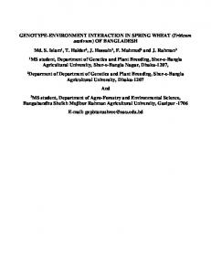
The mean performance of grain yield over environments indicated the relative performance of the genotypes tested across environments (Table 1). The environment mean yield ranged from 541.4 (E17, Shirvan 2003) to 2,024.1 kg ha-1 (E3, Gachsaran 2004) indicating subseasonal differences among test environments. This yield range reflected the different climatic conditions across locations and years. Mean environment yield was positively related to pre-season rainfall (r = 71.3%, P < 0.01) (Table 1). Shirvan 2003 and Gorgan 2002, the lowest yielding environments, had little pre-season and seasonal rainfall, whereas Gachsaran 2004 and Ilam 2002, the highest yielding environments, had much pre-season and seasonal rainfall. Tukey’s one degree of freedom for non-additivy test was used to test for the presence of crossover GE interaction in the two way data. The significance (P < 0.01) of nonadditivity was an indication of a crossover GE interaction. A graph of genotype versus environment mean yield also showed the presence of crossover interaction (Fig. 1).
2,800 2,400 2,000 Mean yield (kg ha–1)
Environments
1,600 1,200 800 400 0 1 2 3 4 5 6 7 8 9 10 11 12 13 14 15 16 17 18 19 20 Environments Genotypes FLIP 97-1L FLIP 82-1L FLIP 92-15L FLIP 96-9L FLIP 92-12L FLIP 96-4L
Stability analyses The results of the different linear regression stability parameters are given in Table 3. Coefficients of regression
ILL 7946 ILL6037 ILL 6199 Gachsaran Kermanshah
Figure 1. Plot of the 11 lentil genotypes versus the environment mean yield to visually assess GE interaction and genotypes stability.
Table 3. Stability parameters, based on regression models, for the 11 lentil genotypes grown in 20 environments Regression stability parametersa
Genotypes Name
FLIP92-12L Gachsaran FLIP 82-1L FLIP 97-1L ILL 7946 ILL 6199 FLIP92-15L ILL 6037 Kermanshah FLIP 96-4L FLIP 96-9L a
Mean yield FW (kg ha–1)
1,376 1,360 1,340 1,197 1,170 1,166 1,155 1,135 1,135 1,092 1,032
1.24 1.44* 1.35* 1.06 1.16 0.69* 1.27 0.65* 0.75 0.68 0.71
ER
PJ
MSPJ
FP
MSFP
D2
R2
α
λ
DI
360,163 868,886 442,200 337,129 390,699 302,310 488,527 168,230 212,285 209,932 212,472
0.24 0.44 0.35* 0.06 0.16 –0.31* 0.27 –0.35* –0.25 –0.33 –0.29
39,449 459,293 70,754 93,472 103,779 218,664 155,062 105,082 105,779 133,042 125,661
1.29 1.29 1.36* 1.09 1.17 0.79 1.32* 0.65* 0.75 0.71 0.80
69,878 600,364 162,036 112,250 140,925 186,540 182,846 127,897 98,358 130,266 103,770
2,086,567 10,757,938 3,246,284 2,358,498 2,906,937 3,944,656 4,307,768 1,891,477 1,942,959 2,398,682 2,279,216
0.89 0.50 0.85 0.72 0.74 0.32 0.69 0.46 0.53 0.43 0.47
0.24* 0.45** 0.36** 0.06 0.16 –0.31** 0.27* –0.36** –0.26* –0.33* –0.29*
10.3** 120** 18.4** 24.5** 27.2** 57.3** 40.6** 27.5** 27.7** 34.8** 32.9**
1,591 1,609 1,574 1,380 1,371 1,286 1,374 1,248 1,265 1,208 1,155
Regression coefficient (FW), deviation from regression (ER), Perkins and Jinks model (PJ), MSPJ (residual mean squares from the regression of Perkin and Jink's model), genotypic stability (D2), Freeman and Perkins method (FP), MSFP (residual mean squares from the regression of Freeman and Perkins's model), α and λ Tai (1971), coefficient of determination (R2) and desirability index (DI). All of the regression deviations were significant at 0.01 level of probability. *, **, significance of regression coefficients from 1, at 0.05 and 0.01 level of probability, respectively.
390
H. Dehghani et al. / Span J Agric Res (2008) 6(3), 385-394
simple linear regression (Eberhart and Russell, 1966) showed that ILL 6037 was a stable genotype which had specific adaptability to poor environments (b = 0.65) but FLIP 82-1L had specific adaptability to favourable environments (b = 1.35). Applying the PJ linear regression model for analyzing the stability of the lentil genotypes studied showed that genotype Gachsaran was stable because of a high regression coefficient and had specific adaptability to favourable environments. The results of the FP regression procedure including regression coefficients and deviation mean square (Table 3) showed that genotype FLIP 82-1L was stable, but genotype ILL 6037 was unstable with specif ic adaptability. The estimates of the parameters αi and λi for seed yield of the genotypes are given in Table 3. The genotypes Gachsaran and FLIP 92-12L were stable based on the α i and λ i parameters, respectively. All genotypes had high λi values. Genotypes FLIP 82-1L, FLIP 92-15L and FLIP 92-12L gave a signif icant positive αi but genotypes FLIP 96-9L, FLIP 96-4L and ILL 6037 gave a significant negative αi. Genotype ILL 6037 had the lowest D2 values and thus was stable, but genotype Kermanshah had the highest D2 values and was unstable. Pinthus’s (1973) stability parameter or coefficient of determination (R2) values for the lentil genotypes tested indicated that genotype FLIP 92-12L was stable and the genotype response to environments is predictable to considerable degree. Results of this parameter were similar to deviation from simple linear regression in the PJ, FP and λi procedures. Genotypes Gachsaran, FLIP 92-12L and FLIP 82-1L had highest
DI values, and were stable, but genotypes FLIP 96-9L, FLIP 96-4L and ILL 6037 were unstable. According to the environmental variance (EV) stability parameter genotypes ILL 6037, Kermanshah, FLIP 96-4L and FLIP 96-9L were more stable and had biological stability (Table 4). The results of the CV stability parameter were similar to the EV statistic and indicated that genotypes ILL 6037 and Kermanshah have a low CV and were stable (Table 4). The W2 values ranged from 932841 for FLIP 92-12L to 9036281 for Gachsaran (Table 4). Genotypes FLIP 92-12L, FLIP 97-1L and FLIP 82-1L had the best stability according to their SH values (Table 4) similar to W2 results where Gachsaran had the lowest stability as well as average yield. Analysis of stability using PP and P parameters gave similar results to the W2 and SH parameters. Table 5 shows that the genotype rank, based on these four stability parameters, was similar and correlation coefficients between these parameters were very high and equal to 1. Lin and Binns (1988) suggested the use of two stability parameters (PI and MSPI) when describing the performance of one genotype across a range of environments. They proposed that the smaller the MSPI the more superior the genotype is and so ranking of the lentil genotypes was done according to both PI and MSPI (not the amounts of the PI itself). In Table 4 the superiority index of the genotypes tested showed FLIP 96-4L and ILL 6199 had the highest stability while applying the MSPI parameter of Lin and Binns (1988) for interpreting of the GE interaction of
Table 4. Variance component stability parameters for 11 lentil genotypes grown in 20 environments Variance component stability parametersa
Genotype Name
FLIP92-12L Gachsaran FLIP 82-1L FLIP 97-1L ILL 7946 ILL 6199 FLIP92-15L ILL 6037 Kermanshah FLIP 96-4L FLIP 96-9L a
Mean yield (kg ha–1)
EV
CV
W2
SH
PP
P
PI
MSPI
1,376 1,360 1,340 1,197 1,170 1,166 1,155 1,135 1,135 1,092 1,032
352,996 863,757 445,090 320,171 375,499 305,779 477,727 185,192 214,399 220,303 223,270
43.19 68.35 49.78 47.29 52.35 47.42 59.82 37.91 40.79 42.99 45.81
932,841** 9,036,281** 1,768,172** 1,697,129** 1,969,156** 4,305,594** 3,072,300** 2,383,238** 2,157,954** 2,802,533** 2,586,407**
40,878** 562,152** 94,612** 90,042** 107,541** 257,838** 178,504** 134,178** 119,686** 161,150** 147,247**
113,086 347,660 137,267 135,211 143,085 210,719 175,018 155,072 148,550 167,209 160,953
185,295 133,168 179,922 180,379 178,629 163,599 171,533 175,965 177,414 173,268 174,658
193,161 176,209 172,597 415,696** 271,360* 535,065** 301,336* 516,799** 40,206* 594,691** 62,727
104,473 80,693 68,288 235,513 75,162 336,095** 95,557 297,771* 183,073 346,048** 334,410**
Environmental variance (EV), coefficient of variability (CV), ecovalance (W2), stability variance (SH), Plaisted and Peterson method (PP), Plaisted procedure (P) and superiority index (PI), MSPI (mean squares of genotype by environment interactions). * and **, significant at the 0.05 and 0.01 probability level, respectively.
GE interaction for grain yield of some lentil genotypes
391
Table 5. Rank of the 11 lentil genotypes grown in 20 environments in Iran, analyzed for stability using 15 univariate methods Genotype
Y
FW
ER
PJ MSPJ FP MSFP
D2
R2
αi
λi
DI
EV
CV
W2
SH
PP
P
PI
MSPI
FLIP92-12L Gachsaran FLIP 82-1L FLIP 97-1L ILL 7946 ILL 6199 FLIP92-15L ILL 6037 Kermanshah FLIP 96-4L FLIP 96-9L
1 2 3 4 5 6 7 8.5 8.5 10 11
4 1 2 6 5 9 3 11 7 10 8
7 11 9 6 8 5 10 1 3 2 4
4 1 2 6 5 9 3 11 7 10 8
3 11 8 5 7 9 10 1 2 6 4
1 7 2 4 3 11 5 9 6 10 8
4 1 2 6 5 9 3 11 7 10 8
1 11 2 3 4 10 9 5 6 8 7
2 1 3 4 6 7 5 9 8 10 11
7 11 9 6 8 5 10 1 2 3 4
4 11 8 6 9 7 10 1 2 3 5
1 11 3 2 4 10 9 6 5 8 7
1 11 3 2 4 10 9 6 5 8 7
1 11 3 2 4 10 9 6 5 8 7
1 11 3 2 4 10 9 6 5 8 7
8 9 10 4 7 2 6 3 5 1 11
5 3 1 7 2 10 4 8 6 11 9
1 11 2 3 4 10 9 5 6 8 7
3.5 3.5 1 6 5 8 2 11 9 10 7
1 11 8 4 7 10 9 5 2 6 3
Yield (Y), regression coefficient (FW), deviation from regression (ER), Perkins and Jinks model (PJ), MSPJ (residual mean squares from the regression of Perkin and Jink's model), Freeman and Perkins method (FP), MSFP (residual mean squares from the regression of Freeman and Perkins's model),genotypic stability (D2), coefficient of determination (R2), α and λ Tai (1971), desirability index (DI), environmental variance (EV), coefficient of variability (CV), ecovalance (W2), stability variance (SH), Plaisted and Peterson method (PP), Plaisted procedure (P) and superiority index (PI). MSPI (mean squares of genotype by environment interactions).
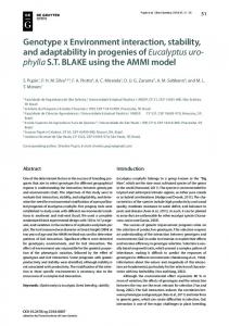
the genotypes tested showed that FLIP 82-1L was stable. The PI index (Table 4) of the genotypes showed FLIP 96-9L and FLIP 82-1L had the highest stability. Applying the MSPI parameter of Lin and Binns (1988) for interpreting GE interaction of the genotypes showed FLIP 82-1L was stable. To reveal associations among genotypes, the twoway data of genotypes, across environments, was analyzed further using a clustering procedure. Ward’s hierarchical clustering indicated that the eleven genotypes could be divided into two major groups (Fig. 2).
The PCA based on correlation matrices was performed to understand the relationship among the different stability parameters. For better visualization, the two first PCs were plotted against each other. The graph of the first two PCs for different stability parameters is shown in Figure 3. The first two PCs explained 92.8% (61.6% and 31.2% by PC1 and PC2, respectively) approximately of the stability methods. Both PC axes of the stability parameters can be divided into f ive distinct classes. In first class (C1) there are eight stability 0.8 MSPI C5
Stability
0.6
Ward’s method
MSPJ C1 PP W2 SH λ P
PI
MSFP2 D
0.4
FLIP 97-1L ILL 6199 FLIP 96-9L FLIP 96-4L ILL 6037 Kermanshah FLIP 82-1L FLIP 92-12L ILL 7946 FLIP 92-15L Gachsaran
0.2
C2 CV EV
Cluster 1
PC2
0.0
ER
–0.2 –0.4
Y
DI FW FP PJ α
–0.6 Cluster 2
R2
–1.0
0
1,000
2,000
3,000 4,000 5,000 Linkage distance
6,000
7,000
Figure 2. Hierarchical cluster analysis of the 11 lentil genotypes based on Ward’s method using a G × E matrix of mean yields.
Yield
C4
–0.8
C3
–1.2 –0.8
–0.6
–0.4
–0.2
0.0
0.2
0.4
0.6
0.8
1.0
1.2
PC1
Figure 3. Plot of the two first PC analyses for mean yield and the 19 univariate methods used to study GE interaction.
392
H. Dehghani et al. / Span J Agric Res (2008) 6(3), 385-394
parameters including the W2, SH, PP, P, λi, MSPJ, MSFP and D2 procedures. The EV, CV and ER procedures are in class 2 (C2). The situation of yield (Y), coefficients of FW, FP, PJ, regression models and DI are in class three (C3), suggesting that selection of the most stable genotypes, based on these parameters, caused high yield genotypes to be introduced as most stable genotypes. Class four (C4) consisted of R2. The PI and MSPI parameters can be classified as class 5 (C5).
Discussion Plant breeders invariably encounter GE interactions when testing varieties across a number of environments. Depending on the magnitude of the interactions or the differential genotypic responses to environment, the varietal rankings can differ greatly across environments. A combined analysis of variance can quantify the interactions, and describe the main effects of years, locations, genotypes and interactions among them. Evaluation of genotypes over several years appears to improve genotype evaluation and it would enable characterization of each genotype for intra-location variance to evaluate the non-predictable part of the GE interactions, due to annual effects (Lin and Binns, 1988). The combined analysis of variance, in this study, was based on random effect of environment (year × location combination) and thus we could not achieve the main effects of year, location and the interaction between them. If the dataset of this investigation was balanced (i.e. the trials of Qazvin location were done for 3 yr), it would be possible to obtain the main effects of year and location. Also, possibly, more information could be gained especially from the year main effect and the interaction of year with other sources of variation. However, analysis of variance is uninformative in the explanation of GE interactions. It seems that other statistical models such as regression procedures are more useful for understanding and describing GE interactions. The GE interaction is an important source of variation in any crop. Geographic differentiation of landraces of lentil emphasizes the specific adaptation of this crop (Erskine, 1997). According to Freeman (1972) one of the main reasons for growing genotypes over a wide range of environments is to estimate their stability and adaptability. The use of two stability parameters may be valuable for some purposes. For a long time, most breeders used the term stability to characterize a genotype which always showed a
constant yield, under variable environmental conditions. This idea of stability agrees with the concept of homeostasis widely used in quantitative genetics and may be considered as a biological (static) concept of stability (Becker and Leon, 1988). Biological stability is not acceptable to most plant breeders, who prefer an agronomic concept of stability. In this concept of stability, it is not necessary for the genotypic response to environmental conditions to be equal for all genotypes. In the graph of the two PCs, the PC1 axis determined the stability methods, which were associated with type 4 (Lin et al., 1986) or the other stability concepts (types 1, 2 and 3). The PC1 axis determined that PI and MSPI were related to the type 4 concept of stability. According to both PCs axes the stability parameters can be divided into four distinct classes. The static stability concept as environmental variance (EV) recognized by Roemer (1917, in Becker, 1981) and generalized by Francis and Kannenberg’s (1978) CV. Figure 3 shows that these methods and the ER method are in class C2. Lin et al. (1986) classified these parameters as stability type 1. The stability statistics of class 1 (MSPJ, MSFP, D 2, W 2, SH, PP, P and λ i) follow the type 2 stability parameters of Lin et al. (1986). Flores et al. (1998) found that the SH, ER and λi methods were related to each other. Kang and Pham (1991) indicated that W 2 showed a stronger correlation with SH. Lin et al. (1986) and Kang et al. (1987) suggested that Wricke’s ecovalance (W2) and stability variance (SH) were the same; stability variance is a coded value of ecovalence, thus these two methods should not be treated as separate procedures. There is also an association between these methods and the P and PP models. In other words, of the 11 statistics mentioned (C1 and C2 classes) follow the biological stability concept and selection of stable genotypes, based on these methods, caused the introduction of stable genotypes that show static stability. Yield (Y) and FW, PJ, FP, DI and α i are in class three (C3), proposing that selection of stable genotypes, based on these procedures, caused high yield genotypes to be introduced as stable genotypes. If selection of stable genotypes was based on these methods, a narrowly adapted genotype with less general adaptability but good specific adaptability may be discarded. However, the PC2 axis distinguishes the stability parameters in C3 that indicate a high association with good yield from stability parameters in C1 and C2 which do not show a relationship with high yield. Stable genotypes based on classes C1 and C2 are suited to unfavourable environments which did
GE interaction for grain yield of some lentil genotypes
not have good edaphic and climatic conditions for sensitive genotypes. The method of Pinthus (1973) can be classified as class four (C4). It was not significantly correlated with the other stability parameters. In this study the stability parameters of different coefficients of simple linear regression showed close relationships with the agronomic concept of stability and high yield. Thus, stable genotypes, according to these statistics, are recommended for favourable environments. In this type of stability a stable genotype showed constant performance across different environments. The two stability parameters of Lin and Binns (1988) did not show any positive correlation with other stability statistics and were grouped as a distinct class (C5). In conclusion, several stability statistics that were used in this study quantified genotype stability with respect to yield. Both yield and stability of performance should be considered simultaneously to exploit the useful effect of GE interactions and to make genotype selection more precise and refined. Genotype FLIP 9212L can be recommended as the most stable genotype with regard to both stability and yield. Genotype FLIP 92-12L was the most stable genotype based on W2, SH, PP, P (Type 2), λi, MSPJ, MSFP stability Type 3 of Lin et al. (1986) and the R2 procedures. This genotype had the highest seed yield among the lentil genotypes studied (1,376 kg ha -1). This genotype is therefore recommended for release as a cultivar by the Dry Land Agricultural Research Institute of Iran.
Acknowledgements The authors are grateful for the support provided by Dry Land Agricultural Research Institute of Iran. Thanks to Prof. A. Bjornstad (Department of Horticulture and Crop Science, Agricultural University of Norway) for providing the SAS programs, needed for this research. We thank two anonymous reviewers of Spanish Journal of Agricultural Research for their helpful comments, suggestions, and corrections of the manuscript.
References BECKER H.C., 1981. Correlations among some statistical measures of phenotypic stability. Euphytica 30, 835-840. BECKER H.C., LEON J., 1988. Stability analysis in plant breeding. Plant Breed 101, 1-23.
393
CECCARELLI S., ERSKINE W., HAMBLIN J., GRANDO S., 1994. Genotype by environment interaction and international breeding programs. Exp Agric 30, 177-188. DELACY I.H., BASFORD K.E., COOPER M., BULL J.K., MCLAREN C.G., 1996. Analysis of multi-environment trail an historical perspective. In: Plant adaptation and crop improvement (Cooper M., Hammer G.L., eds). CAB International: Wallingford, UK. pp.39-124. DUARTE J.B., ZIMMERMANN M.J., 1995. Correlation among yield stability parameters in common bean. Crop Sci 35, 905-912. EBERHART S.A., RUSSELL W.A., 1966. Stability parameters for comparing varieties. Crop Sci 6, 36-40. ERSKINE W., 1997. Lessons for breeders from land races of lentil. Euphytica 93, 107-112. FAO, 1990. Guidelines for soil profile description. 3 rd ed (revised). Soil Resources, Management and Conservation Service, Land and Water Development Division, FAO, Rome, Italy. FAO, 2006. Data stat year 2006. Food Agriculture Organization, Rome, Italy. FINLAY K.W., WILKINSON G.N., 1963. The analysis of adaptation in a plant breeding programme. Aust J Agric Res 14, 742-754. FLORES F., MORENO M.T., CUBERO J.I., 1998. A comparison of univariate and multivariate methods to analyze environments. Field Crops Res 56, 271-286. FRANCIS T.R., KANNENBERG L.W., 1978. Yield stability studies in short-season maize: I. A descriptive method for grouping genotypes. Can J Plant Sci 58, 1029-1034. FREEMAN G.H., 1972. Statistical methods for the analysis of genotype × environment interactions. Heredity 29, 339-351. FREEMAN G.H., PERKINS J.M., 1971. Environmental and genotype-environmental components of variability VIII. Relations between genotypes grown in different environments and measures of these environments. Heredity 27, 15-23. GENSTAT, 2004. GenStat Committee 7 release 1 Reference Manual. Clarendon Press, Oxford, UK. HANSON W.D., 1970. Genotypic stability. Theor Appl Genet 40, 226-231. HERNÁNDEZ C.M., CROSSA J., CASTILLO A., 1993. The area under the function: an index for selecting desirable genotypes. Theor Appl Genet 87, 409-415. JONES M.J., SINGH M., 2000. Long-term yield patterns in barley-based cropping systems in northern Syria. 2. The role of feed legumes. J Agric Sci 135, 237-249. KANG M.S., MILLER J.D., DARRAH L.L., 1987. A note on relationship between stability variance and ecovalence. Heredity 78, 107-112. KANG M.S., PHAM H.N., 1991. Simultaneous selection for high yielding and stable crop genotypes. Agron J 83, 161-165. LIN C.S., BINNS M.R., 1988. A superiority measure of cultivar performance for cultivar × location data. Can J Plant Sci 68, 193-198.
394
H. Dehghani et al. / Span J Agric Res (2008) 6(3), 385-394
LIN C.S., BINNS M.R., LEFKOVITCH L.P., 1986. Stability analysis: where do we stand? Crop Sci 26, 894-900. PERKINS J.M., JINKS J.L., 1968. Environmental and genotype-environmental components of variability. Heredity 23, 339-356. PINTHUS J.M., 1973. Estimate of genotype value: a proposed method. Euphytica 22, 121-123. PLAISTED R.L., 1960. A shorter method for evaluating the ability of selections to yield consistently over locations. Am Potato J 37, 166-172. PLAISTED R.I., PETERSON L.C., 1959. A technique for evaluating the ability of selection to yield consistently in different locations or seasons. Am Potato J 36, 381-385. SABAGHPOUR S.H., SAFIKHNI M., SARKER A., GHAFFRI A., KETATA H., 2004. Present status and future prospects of lentil cultivation in Iran. Proc 5th European Conference on Grain Legumes, 7-11 June, Dijon, France.
SARKER A., ERSKINE W., SINGH M., 2003. Regression models for lentil seed and straw yields in Near East. Agr Forest Meteorol 116, 61-72. SAS INSTITUTE, 1996. SAS/STAT User’s Guide. 2 nd ed. SAS institute Inc., Cary, NC, USA. SHUKLA G.K., 1972. Some statistical aspects of partitioning genotype-environmental components of variability. Heredity 29, 237–245. SPSS Inc, 2004. SPSS 14. SPSS User’s guide. SPSS Inc, Chicago, IL. USA. TAI G.C.C., 1971. Genotypic stability analysis and application to potato regional trials. Crop Sci 11, 184-190. WRICKE G., 1962. Über eine Methode zur Erfassung der ökologischen Streubreite in Feldversuchen. Z Pflanzenzücht 47, 92-96. [In German]. YATES F., COCHRAN W.G., 1938. The analysis of groups of experiments. J Agric Sci 28, 556-580.