Supplement of Clim. Past, 12, 387-414, 2016 http://www.clim-past.net/12/387/2016/
Geochronological database and classification system for age uncertainties in Neotropical Pollen records Supplementary information Version 2 Suzette G.A. Flantua, Maarten Blaauw, Henry Hooghiemstra
[email protected] [email protected]
Introduction This document presents the outcomes and the manual of the methodology presented in the paper “Geochronological database and classification system for age uncertainties in Neotropical Pollen records” by S.G.A. Flantua, M. Blaauw and H. Hooghiemstra and in Clim. Past. 12, 387-414, 2016 http://www.clim-past.net/12/387/2016.
The methodology uses the R-code called ‘Clam’ to perform age-depth modelling for palaeoecological records (in this case pollen records) and implements an adjusted version from the ‘star classification system’ presented in Giesecke et al. (2014). This star classification is displayed along a site’s age model to indicate age uncertainty.
This document has been structured in two parts: 1) Outcomes from Flantua, Blaauw and Hooghiemstra (2016). 2) Setup of the programs and the scripts or “codes” to produce new age models with star classification outcome. This is the Version II of this manual, uploaded September 2017. We will aim to update this manual when further improvements are needed. If you have any questions or comments, please don’t hesitate to contact us. We would be happy to hear from you.
Suzette Flantua:
[email protected] Maarten Blaauw:
[email protected]
1
1. Outcomes from Flantua, Blaauw and Hooghiemstra (2016). 1)
From
http://dx.doi.org/10.6084/m9.figshare.2069722.v2
download
the
folder
called
Flantua_ClimPast_2016.zip.
This
folder
contains
the
original
publication
“Flantua,
Blaauw,
Hooghiemstra_2016_CP_AgeModelling.pdf”, the table with the list of sites used “LIST_sites.xlsx”, the literature list from these sites “LIST_publications_from_sites.xlsx” and the folder “Cores” with the recalibrated age models from this paper and the corresponding folder with all the descriptions. The text file “script_per_agemodel_FINAL” contains the parameters used for each age model in the R scripts.
Open “LIST_sites.xlsx”. The first column indicates the identification number that concurs with the numbers in the folder “Cores”. The last column indicates the reference you will find in the file “LIST_publications_from_sites.xlsx”. In the latter, you will obtain the complete reference organized in alphabetic order.
2
Open the folder “Cores” in your file browser. Here you will find for each core (analyzed pollen record) the age models as present in the “LIST_sites.xlsx”. Open folder “0309_CTY1”. Here you find the folders of the different age models. Open folder “Run8”. You will find the different files that served as input and the files that were produced as output. In the following Table 1 each file is explained in more detail. All .txt and .csv files can be opened in a plain-text editor such as WordPad. As you will see, each run will always have an age model produced by linear interpolation and in case that more than three control points were available (e.g. 14C data points), also a smooth spline age model.
Table 1. Age model files FILE NAME
EXPLANATION
0309_author_depths.csv
Csv (comma-separated value)-file with the sample depths.
0309_CTY1.csv (input)
‘Control point file’: File with the data on the control points (such as
14
C), error, reservoir, depth, thickness
and RCode (Codes explained in Table 2). This is one of the basic files required to run ´Clam´. 0309_CTY1_depths.txt (input)
Text file with the sample depths. This is one of the basic files required to run ´Clam´.
0309_CTY1_calibrated.txt (output)
File with the calibrated age ranges at 95% confidence interval.
0309_CTY1_interpolated.pdf (output)
Generated age model based on interpolation, pdf format.
0309_CTY1_interpolated.png (output)
Generated age model based on interpolation, png format.
0309_CTY1_interpolated_ages.txt (output)
Calibrated ages for each sample depth based on interpolation. From left to right: depths, minimum calibrated age, maximum calibrated age, “best” age, estimated accumulation rate.
0309_CTY1_interpolated_settings.txt (output)
Parameters used to produce the interpolated age model, such as calibration curve used, modeling
3
method and goodness-of-fit. 0309_CTY1_interpolated_stars.txt (output )
Outcome from the star classification system based on interpolation.
From
left
to
right:
sample
depth,
[constant] star assigned when a segment is straight, [bad.extra] stars assigned when maximum distance to nearest date (yr) = 2000, [good.extra] max. distance to nearest date (yr) = 1000, [best.extra] max. distance to nearest date (yr) = 500, [stars] total number of stars. 0309_CTY1_old.csv
Reference file indicating depths and control points with top (TOP) and bottom (BOT).
0309_CTY1_smooth_spline.pdf (output)
Generated age model based on smooth spline, pdf format.
0309_CTY1_smooth_spline.png (output)
Generated age model based on smooth spline, png format.
0309_CTY1_smooth_spline_ages.txt (output)
Calibrated ages for each sample depth based on smooth spline. From left to right: depths, minimum calibrated age, maximum calibrated age, “best” age, estimated accumulation rate.
0309_CTY1_smooth_spline_settings.txt
Parameters used to produce the smooth spline age
(output)
model, such as calibration curve used, modeling method and goodness-of-fit.
0309_CTY1_smooth_spline_stars.txt (output)
Outcome from the star classification system based on smooth spline. From left to right: sample depth, [constant] star assigned when at straight
segment,
[bad.extra] stars assigned when maximum distance to nearest date (yr) = 2000, [good.extra] max. distance to nearest date (yr) = 1000, [best.extra] max. distance to nearest date (yr) = 500, [stars] total number of stars. 0309_CTY1_smoothspline.pdf (output)
Generated age model based on smooth spline with the star classification result plotted along the vertical axis, pdf format.
4
Table 2. Description of “RCode” in control point file RCODE
DESCRIPTION
PB2
210Pb
C14
Carbon-14 or Carbon-14: AMS
BEN
Compared with benthic oxygen isotope data
BOT_C
Core base estimated
BOT_A
Core base known
BOT_U
Core base unknown
TOP_C
Core top estimated
TOP_A
Core top known
TOP_U
Core top unknown
Fision
Fission track
LS
Liquid scintillation
TEF
Tephra
TL
TL-date
U238
Uranium series
DER
Age derived from known event
Descriptions of the original and recalibrated age models (folder “Descriptions age models”) As mentioned previously, each document provides the metadata of the pollen record (site name and original publications), important observations on the original age model, and the newly calibrated age model by Flantua, Blaauw and Hooghiemstra (2016). We did not include figures and tables from the original age models due to copyright issues, but this information has been collected as well for comparison. The document furthermore mentions if an original depths file was available (the exact depths at which samples were taken) or if depths were derived from the original publications. For each record different age models were created to compare the effect of including e.g. an outlier, a hiatus and/or estimated top age. In the description there will be an explanation of the ‘runs’ 1 executed and the differences between them in terms of the used parameters The last model in consecutive order (e.g. run 9 vs run 8) is generally the one considered with the best fit. The outcomes are all found in the corresponding folders of the records in the folder ‘Cores’ within the folder “Flantua_ClimPast_2016” and the text file “script_per_agemodel_FINAL” includes the parameters for each age model as used in R (explained later on in this manual).
1
With a ‘run’ is meant the execution of the R codes presented in this manual.
5
2. Setup of the programs and codes. Here we will explain the basics of running Clam to make an age model for your own record and how to obtain the star classification output alongside.
Required programs 1) R: You need to have installed a recent version of the free open-source statistical software R (R Core Team, 2015). This program is needed to run the different codes from this manual. To obtain the latest version of R, please access https://www.r-project.org/. R runs on a wide range of operating systems including Windows and Mac. Install the program as you would with any other program. 2) Clam.R: Clam is a code that will run in R. Therefore, it has the extension “.R”. With this code you will be able to perform ‘classical’ age-depth modelling (Blaauw, 2010), which is different to the flexible Bayesian age-depth modelling performed by the code called Bacon (Blaauw and Christen, 2011). Here we only use Clam. To obtain the latest version of Clam, go to http://chrono.qub.ac.uk/blaauw/Clam.html There you will also find the extensive version of the manual on Clam. 3) StarClassification_AgeModels.R: This is also an R-code and in this case needed to perform the star classification system on the age models.
Install programs 1) From the figshare link http://dx.doi.org/10.6084/m9.figshare.2069722.v2, download the file called Clam_Stars.zip. Unzip to somewhere on your computer where you have write access (e.g. d:\Clam_Stars).
2) In this folder you will find three R-codes and the different calibration curves available to create age models. The calibration curves are in a format “14C file”. Furthermore there is a folder called ‘Cores’ that contains two examples to run the scripts before preparing your own data. This folder contains the different files needed to run the age model, such as the 14C data and sample depths (See the ´input´ files in Table 1). This will be explained in further detail in the next section.
6
How to access and run the codes Open R Change the working directory to the Clam_Stars folder (e.g. d:\Clam_Stars). Load the R-code Clam so to enter the age modelling program as followed: o
Write: source ("Clam.R")
o
Enter
o
Output: > “Hi there, welcome to Clam for age-depth modelling.”
To
run
the
star
classification
system,
you
have
to
load
the
R-code
called
‘StarClassification_AgeModels.R’ o
Write: source ("StarClassification_AgeModels.R")
o
Enter
o
No output will be shown, but the code is now loaded.
R is now ready to use Clam to create an age model and to implement the star classification system to define age uncertainty for each sample.
7
Note The R codes and the ‘Cores’ folder always need to be organized together as shown in the figure above and names of files and folders should not be changed. In the Clam_Stars folder there is a R-code called “Script_per_AgeModel.R”. You can open this code in RStudio or with the program Notepad. You will see two commands starting with “Agemodel.stars”, then the identification of the core (e.g. “0309_CTY1”) and what follows are the parameters to define additional features of the age model. In this case: Agemodel.stars("0309_CTY1", cc=3, smooth=0.3
Here below we first explain the parameters we have been using for the age models, e.g. type of calibration curve, outliers and hiatus.
Parameters to define your age model For each age model you want to create, you need to specify the parameters. For several parameters, there is already a default value defined in Clam (see the manual of Clam for additional information on these default values: http://chrono.qub.ac.uk/blaauw/Clam.html).
Calibration curves To define which calibration curve needs to be implemented, the term ‘cc’ is used e.g. Agemodel.stars("0893_FUQ3", cc=1). By default the northern hemisphere terrestrial calibration curve is used (Table 3). To use alternative curves, change the value of ´cc´ to the number of the desired calibration curve (e.g. cc=2). Table 3. Calibration curves and number Calibration curve
Number
IntCal13.14C
1
Marine13.14C
2
SHCal13.14C
3
Postbomb calibration curve Negative radiocarbon ages are calibrated using postbomb curves and the user needs to inform Clam which curve to use. If no postbomb option is provided for cores with negative radiocarbon ages, Clam will not
8
produce an age-depth model. To know which postbomb calibration curve to use (Table 4), there is a world map presented in Hua et al. (2013). When the appropriate postbomb curve is identified, this can be specified
in
the
R-code
“script_per_agemodel.R”
by
the
expression
‘postbomb’,
e.g.
Agemodel.stars("0394_TQMA", cc=3, postbomb=5). In this example, postbomb curve SH3.14C is used.
Table 4. Postbomb calibration curves and number
Postbomb calibration curve
Number
postbomb_NH1.14C
1
postbomb_NH2.14C
2
postbomb_NH3.14C
3
postbomb_SH1-2.14C
4
postbomb_SH3.14C
5
Hiatus A core can have a hiatus (a missing section in the core) at a certain depth or even multiple ones. In some cases this can be important to include in the age depth model. The expression ‘hiatus’ is used as followed: ‘hiatus=470’ meaning that there is hiatus at 470 cm depth, or in case of multiple ones: ‘hiatus = c(470,600)’ (hiatus at 470 cm and 600 cm depth). In “script_per_agemodel.R” it will look like this: Agemodel.stars("0907_JOTAR", cc=1, postbomb=2, hiatus=c(410))
Slump A slump can occur when a mass movement of sediment is introduced into the record. On some cases this can be important to include in the age depth model. For the expression ‘slump’ you need to define the upper and lower depths, e.g. slump=c(470,600) when there is a slump at 470 cm depth, or in case of multiple ones: ‘slump = c(80,100,470,600)’ (slump between 80 cm and 100 cm depth, and between 470 and 600). In “script_per_agemodel.R” it will look like this: Agemodel.stars("0875_BOSQ1", cc=1, slump=c(72,90)).
Outliers Control dates may be considered as outliers due to recent contamination or mixing of sediment, among others. The outliers are marked in Clam by the expression ‘outliers’ and their position within the control
9
point file should be indicated counting from the top of the sequence. For example, in case that the second date in 0309_CTY1.csv (input) would be the outlier (3095 14C yr), then the expression in “script_per_agemodel.R” will become: Agemodel.stars("0309_CTY1", cc=3, outliers=c(2)).
Smoothness of smooth spline age model The R-code to implement the star classification system will always try to produce two types of age models. The linear interpolation or regression needs at least two control points and the smooth spline at least four data points. The smoothness of the smooth spline can be adjusted by using the expression “smooth”. The default value is 0.3. To produce an age model with a “stiffer” smoothness (for example to avoid age reversals) higher values should be used, e.g. smooth=0.5. For a more flexible smooth spline (for example to better “fit” dispersed dates), lower values can be used, e.g. smooth=0.15. In “script_per_agemodel.R” it will look like this: Agemodel.stars("0333_LKAT", cc=3, smooth=0.22).
Organizing the input file Within the folder ‘Cores’ you will find two folders from two different records, namely 0309_CTY1 and 0310_CTY2.
Within each folder you will find two input files that start with exactly the same name as the folder. This is very important that the name of the folder is EXACTLY the same as the files within the folder, or else clam will give you an error and will not produce any age model. The two files in each folder are the two necessary input files as described in Table 1.
The input files 1)
The ‘Control point file’: File with the data on the control points and corresponding information.
2)
Depth-file. The file with the depths at which samples were taken.
How to make a Control point file: 1) Open Excel to make the control point file. 2) This file has 8 columns of information of which 7 are read by Clam.
10
Table 5. Postbomb calibration curves and number
1
HEADER
INFORMATION
ID
Identification codes of each control points, such as laboratory code. Both letters and numbers may be used.
2
C14_age
Uncalibrated age of control point, such as the 14C age or the tephra age as measured by the laboratory. Units are in years before present.
3
Cal_BP
This column is most often left open because Clam calculates the calibrated ages itself. This column can be used if you want to include the estimated top or bottom age, for example by “0” or ”-60” to indicate that top section is ´recent´. Only provide a year before present (cal yr BP), because text characters, e.g., "AD 1900" or "1900-1950" for a calendar age cause problems.
4
error
Error of the uncalibrated age of control point, e.g. “150” for 150 years. Errors should always be greater than 0.
5
reservoir
If the age offset due to the reservoir effect is known, then include here.
6
depth
Depth as which the control point is taken. Units are in cm, e.g. “28” for 28 cm. This column should never be left open.
7
thickness
The thickness of the sample to derive the control point, e.g. “5” for 5 cm. The default thickness is 1 cm and will obtain this value when this column is left open.
8
RCode
(optional) An additional column used to include a code on the control point, such as 14C for a
14
C date, TOP_C for an estimated top age, or TEF for a
tephra age. Additional options are shown in Table 2.
Notes: Name the columns exactly in the same order and with the same name as described in Table 5. Order the dates according to their depths, starting with the highest dates and working downwards. Do not use commas as decimals separators but dots. This file should be in csv-format. Use the function “Save as” to replace the Excel file (in case you use Excel) by csv. The .csv file can be opened in a plain-text editor such as WordPad or NotePad to quickly check for and correct any errors (e.g. removing empty rows with lots of commas).
Click “Save as type” and look for “CSV (Comma delimited) (*.csv)”
11
Depth file: This file is a simple text file that should only have the list of depths in cm at which samples were taken. Do not include a header like “depths (cm)”, only the values of the depths. This file should have exactly the same name as the folder including “_depths”.
Organization of the folders and files Make sure that you have everything organized as shown in the folder ‘Clam_stars’. This means having the 14C files together with the R files and the folder ‘Cores’ with the folder with your site information.
12
To run clam and the star classification system for ONE age model When you are ready with defining your parameters and you have your folders ready, let’s say in this case Agemodel.stars("0310_CTY2", cc=3, smooth=0.2), you can paste this directly into R Console (where you write your commands where the >
symbol is). By pressing ‘Enter’, clam.R and
StarClassification_AgeModels.R will run and produce the output within the folder you have destined to your record, in this case folder “0310_CTY2”. All output files as specified in Table 1 will be produced.
To run clam and the star classification system for MANY age models For running many age models at a time, it’s useful if you use a R-code where the parameters from each record are joined and clam will run through all of them to produce age models. For this purpose, the file “script_per_agemodel.R” can be used to run several age models at a time.
In this example, the file “script_per_agemodel.R” contains the commands for two records, 0309_CTY1 and 0310_CTY10. To tell Clam that it needs to read the R-code “script_per_agemodel”: o
Write in R Console: source “script_per_agemodel.R”
o
Output: Each core folder will now contain the age models with the star classification output (see Table 1).
For your own age models: You can paste the commands for each separate age model directly in script_per_agemodel.R (e.g. if you have it open in RStudio. Don’t forget to save!) or you can use Notepad to make adjustments and then save back to an R-file. When you used Notepad, simply save “script_per_agemodel.R” as text. Now change the extension (e.g. by using Windows Explorer) from “.txt” to “.R”, to convert it into a R file. Now the file is ready to be read by Clam.
NOTE: Each time you run Clam reading the “script_per_agemodel.R” file, the files within the folder ‘Cores’ will be overwritten. So all the output files from Table 1 will be overwritten. If you would like to save those output files, move the output files to another folder but take care that you leave the input files for Clam to read.
13
REFERENCES
Blaauw, M. and Christen, J. A.: Flexible paleoclimate age-depth models using an autoregressive gamma process, Bayesian Anal., 6(3), 457–474, doi:10.1214/ba/1339616472, 2011.
Flantua, S.G.A., Blaauw, M. and Hooghiemstra, H.. 2016. Geochronological database and classification system for age uncertainties in Neotropical Pollen records. Clim Past 12, 387-414, www.climpast.net/12/387/2016/
Giesecke, T., Davis, B., Brewer, S., Finsinger, W., Wolters, S., Blaauw, M., Beaulieu, J.-L. de, Binney, H., Fyfe, R. M., Gaillard, M.-J., Gil-Romera, G., van der Knaap, W. O., Kuneš, P., Kühl, N., van Leeuwen, J. F. N., Leydet, M., Lotter, A. F., Ortu, E., Semmler, M. and Bradshaw, R. H. W.: Towards mapping the late Quaternary vegetation change of Europe, Veget Hist Archaeobot, 23(1), 75–86, doi:10.1007/s00334-012-0390-y, 2014.
Hua, Q., Barbetti, M. and Rakowski, A. Z.: Atmospheric radiocarbon for the period 1950–2010, Radiocarbon, 55(4), 2059–2072, 2013.
R Core Team. R: A language and environment for statistical computing. R Foundation for Statistical Computing, Vienna, Austria. https://www.R-project.org/, 2015.
14