Geodesic Convolutional Shape Optimization - arXiv

Geodesic Convolutional Shape Optimization

Pierre Baque * 1 Edoardo Remelli * 1 Franc¸ois Fleuret 2 1 Pascal Fua 1

arXiv:1802.04016v1 [cs.CE] 12 Feb 2018

Abstract Aerodynamic shape optimization has many industrial applications. Existing methods, however, are so computationally demanding that typical engineering practices are to either simply try a limited number of hand-designed shapes or restrict oneself to shapes that can be parameterized using only few degrees of freedom. In this work, we introduce a new way to optimize complex shapes fast and accurately. To this end, we train Geodesic Convolutional Neural Networks to emulate a fluidynamics simulator. The key to making this approach practical is remeshing the original shape using a poly-cube map, which makes it possible to perform the computations on GPUs instead of CPUs. The neural net is then used to formulate an objective function that is differentiable with respect to the shape parameters, which can then be optimized using a gradient-based technique. This outperforms stateof-the-art methods by 5 to 20% for standard problems and, even more importantly, our approach applies to cases that previous methods cannot handle.

1. Introduction Optimizing the aerodynamic or hydrodynamic properties is key to designing shapes, such as those of aircraft wings, windmill blades, hydrofoils, car bodies, bicycle shells, or submarine hulls. However, it remains challenging and computationally demanding because existing Computational Fluid Dynamics (CFD) techniques rely either on solving the Navier-Stokes equations or on Lattice Boltzmann methods. Since the simulation must be re-run each time an engineer wishes to change the shape, this makes the design process slow and costly. A typical engineering approach is therefore to test only a few designs without a fine-grained search in the space of potential variations. *

Equal contribution 1 CVLab, EPFL, Lausanne, Switzerland Machine Learning Group, Idiap, Martigny, Switzerland. Correspondence to: Pierre Baque . 2

Xtrain

Fωy (Xtrain )

Fωz (Xtrain )

Fωy (Xtest )

Fωz (Xtest )

GCNN (a)

Xtest GCNN

(b)

(c)

G(X) −∇X G

−∇X G G(X)

G(X)

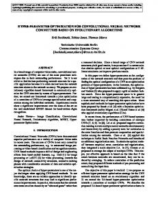
Figure 1. Car shape optimization. (a) We train a GCNN to emulate a CFD simulator and predict from the shape on the left pressures shown as colors in the middle and drag shown as a gray vertical bar on the right. (b) Convolutional layers enable the GCNN to make accurate predictions on previously unseen shapes, such as those of cars. (c) We use the GCNN to express drag as a differentiable function of the mesh vertex positions. Finally, we minimize it under constraints to produce the rightmost shape.

This is a severe limitation and there have been many attempts at overcoming it, but none has been entirely successful yet. Most current algorithms rely on combining evolutionary algorithms with heuristic local search (Orman & Durmus, 2016) and complex adjoint methods (Allaire, 2015; Gao et al., 2017), which requires rerunning a simulation at each iteration step and therefore remains costly. A classical approach to reduce the computational complexity is to use Gaussian Process (GP) regressors trained to interpolate the performance landscape given a low dimensional parametrization of the shape space. This interpolator is then used as a proxy for the true objective to speed-up the computation, which is referred to as Kriging in the CFD literature (Toal & Keane, 2011; Xu et al., 2017). However, those regressors are only effective for shape deformations that can be parameterized using relatively few parameters (Bengio et al., 2006) and their performance therefore hinges on a well-designed parameterization. Furthermore, the regressors are specific to a particular parameterization and pre-existing computed simulation data using different ones cannot be easily leveraged. By contrast, we propose an approach to optimizing the aero-

Geodesic Convolutional Shape Optimization

dynamic or hydrodynamic properties of arbitrarily complex shapes by training Geodesic Convolutional Neural Networks (GCNNs) (Monti et al., 2016) to emulate a fluidynamics simulator. More specifically, given a set of generic surfaces parametrized as meshes, we train a GCCN to predict their aerodynamic characteristics, as computed by standard CFD packages, such as XFoil (Drela, 1989) or Ansys Fluent (Inc., 2011), which are then used to write an objective function. Since this function is differentiable with respect to the vertex coordinates, we can use it in conjunction with a gradientbased optimization to explore the shape space much faster and thoroughly than was possible before, with a much better accuracy and without putting undue restrictions on the range of potential shapes. Since performing convolutions on an arbitrary mesh is much slower than on a regular grid, the key to making this approach practical is remeshing the original shape using a cube or poly-cube map (Tarini et al., 2004). It makes it possible to perform the GCNN computations on GPUs instead of CPUs, as for normal CNNs. In short, our contribution is a new surrogate model method for shape optimization. It does not rely on handcrafted features and can handle shapes that must be parameterized using many parameters. Since it operates directly on the 3D surfaces, an added benefit is that it can leverage training data produced using any kind of parameterization and not only the specific one used to perform the shape optimization. Fig 1 illustrates the process. The training shapes can be very different from the target one, which gives our system flexibility. We demonstrate that our method outperforms GP approaches, widely used in the industry, both in terms of regression accuracy and optimization capacity. Not only do we improve upon GP optimization by 5% to 20% for a lift maximization task on 2D NACA airfoils involving few parameters, but we can also deliver results on fully 3D shapes for which our baselines perform poorly.

2. Related Work There is a massive body of literature about fluid simulation techniques. Traditional ones rely on numerical discretization of the Navier-Stokes Equations (NSE) using finitedifference, finite-element, or finite volume methods (Quarteroni & Quarteroni, 2009; Skinner & Zare-Behtash, 2018). Since the NSE are highly non-linear, the space has to be very finely discretized for good accuracy, which tends to make such methods computationally expensive. In some cases, approaches such as the Lattice-Boltzmann Method (LBM) (McNamara & Zanetti, 1988), which simulates streaming and collision processes across individual fluid particles to recover the global behavior as an emergent property, can be more accurate, at the cost of being even more computationally expensive (Xian & Takayuki, 2011).

All the above-mentioned techniques approximate the fluodynamics for a fixed physical shape and without changing it. A common engineering practice is therefore to first use them to compute the characteristics of a few hand-designed shapes and then to pick the one giving the best results. In this paper, our focus is on using a Deep Learning approach to automate this process by casting it as a gradient descent minimization. In the remainder of this section, we therefore review existing approaches to shape optimization in the CFD context and then discuss current uses of Deep Learning in that field. 2.1. Shape Optimization A popular and relatively easy to implement approach to shape optimization relies on genetic algorithms (Gosselin et al., 2009) to explore the space of possible shapes. However, since genetic algorithms require many evaluation of the fitness function, a naive implementation would be inefficient because each one requires an expensive CFD simulation. This can be avoided using Adjoint Differentiation (Allaire, 2015; Gao et al., 2017) instead. It involves approximating the solution of a so-called adjoint form of the NSE to compute the gradient of the fitness function with respect to the 3D simulation mesh parameters. This allows the use of gradient-based optimization techniques but is still very expensive because it requires a new simulation to be run at each iteration (Alexandersen et al., 2016). As a result, there has been extensive research in ways to reduce the required number of evaluations of the fitness function. One of the most widely used one relies either on Gaussian Processes (GPs, Rasmussen & Williams, 2006), which is known as kriging in the CFD community (Jeong et al., 2005; Toal & Keane, 2011; Xu et al., 2017), or on Artificial Neural Networks (ANN, Gholizadeh & Seyedpoor, 2011; Lundberg et al., 2015; Preen & Bull, 2015) to compute surrogates or meta-models that approximate the fitness function while being much easier to compute. Both approaches can be used either to simply speed-up genetic algorithms (Ulaganathan & Asproulis, 2013) or to find an optimal trade-off between exploration and exploitation, using the confidence bounds provided by the GPs to optimize a multi-objective Pareto front. However, these methods all depend on handcrafted shape parameterizations that can be difficult to design. Furthermore this makes it necessary to retrain the regressor for each new scenario in which the parameterization changes. 2.2. Deep Learning As in many other engineering fields, Deep Learning was recently introduced in CFD. For example, Neural Networks are used by Tompson et al. (2016) to accelerate Eulerian fluid simulations. This is done by training CNNs to approxi-

Geodesic Convolutional Shape Optimization

mate the solution of the the discrete Poisson equation, which is usually the most time demanding step in an Eulerian fluid simulation pipeline. Along similar lines, 3D CNNs are used by Guo et al. (2016) to directly regress the fluid velocity field at every point of the space given an implicit surface description of the target object. These two methods demonstrate the potential of Deep Learning to speed-up and reproduce fluid simulations. However, they rely on 3D CNNs which have a large memory footprint and are extremely computationally demanding whereas the object of interest is intrinsically represented as 2D manifold. This can be mitigated by running the simulations over a coarse space discretization, which degrades the accuracy. By contrast, our proposed approach directly runs on a surface mesh representation of the object, which enables us to use one less dimension and thus considerably reduce the computing requirements.

3. Regression of physical quantities We define the set of meshes M ⊂ R3N × {0, 1}N ×N and M = (X, E) ∈ M , a mesh as being a pair composed of locations of vertices, and their connectivity. Let us assume we are given a set of meshes Mm = (Xm , Em ), m = 1, . . . , M, and let us further assume that for each one, we ran a CFD solver to compute both a corresponding vector of local physical quantities Ym ∈ RN , one for each vertex, along with a global scalar value Zm ∈ R. Concretely, Ym could be the air-pressure field along a plane’s wing and Zm the total drag force it generates. From these values we can infer a performance score, such as Liftto-Drag ratio for a wing, using a differentiable mapping. Given M such triplets (Mm , Ym , Zm ), we want to train a regressor Fω : M → RN × R such that Fω (Mm ) = (Fωy (Mm ), Fωz (Mm )) ≈ (Ym , Zm ) ,

(1)

where ω comprises the trainable parameters, which will be optimized to minimize our training loss X 2 L(ω) = kFωy (Mm )−Ym k2 +λ (Fωz (Mm )−Zm ) , (2)

described by Monti et al. (2016) instead. These explicitly account for the varying geodesic distances between vertices when performing convolutions. However, the structure of the input – the fact that it is organised as a tensor where adjacent elements are neighbours in the physical world–, is also central to the efficient use of modern computational hardware and results in speed-up of several orders of magnitude. For our application, the lack of structure of arbitrary surface meshes – often composed of triangles – would slow down the computation and prevent effective use of the GPUs for a naive implementation of GCNNs. In this section, we first introduce GCNNs which help overcome the first difficulty and then show how we can remesh the surface into a quad-mesh to tackle the second one. Geodesic CNNs. We describe the geometric convolution operation that is used at each vertex, where a mixture of gaussians is used to interpolate the features computed at neighbouring vertices into a common predefined basis. Let us consider a signal f = (f 1 , . . . , f N ) defined at each one of the N vertices Xi 1≤i≤N of mesh M. For each i, let N i = {j : E(i, j) = 1}, that is the set of indices j such that Xi and Xj are neighbors. Let K, where K = 32 in all our experiments, be a predefined number of gaussian parameters αk ∈ R2 , Σk ∈ R2 , which are vertex independent. We can now define an interpolation operator Dk over the mesh vertices by writing i

(Dk f ) =

X j∈N i

 −(ρ(Xi , Xj ) − αkρ )2 f exp Σkρ   −(θ(Xi , Xj ) − αkθ )2 exp , (3) Σkθ j



where ρ(·) and θ(·) are relative geodesic coordinates. This makes it possible to define the convolution of f by a filter g over the mesh as X f ?g = gk Dk f. (4) k∈1,...,K

m

where λ is a scaling parameter that ensures that both terms have roughly the same magnitude. 3.1. From Geodesic to Cube-Mesh CNNs Standard CNNs implicitly rely on their input, images usually, having a regular Euclidean geometry. The neighborhood relationship between pixels encodes their distance. While such a regularity is true for images, it is not for surface meshes. To operate on such an input, one therefore should use Geodesic CNNs (GCCNs) such as those

This operator can then be used as a building block for a convolutional architecture. The learning phase involves a gradient-descent based optimization of the convolutional function parameters gk , as in standard CNNs. The values of αk and Σk can be set manually and kept fixed during training (Kipf & Welling, 2016). However, it is more effective to learn them (Monti et al., 2016). Unfortunately, the meshes we must deal with are typically large and a naive implementation of the GCNNs would be prohibitively expensive because the convolution of Eq. 3 lacks the structure that would make it easy to implement

Geodesic Convolutional Shape Optimization (a)

volumetric deformation

(b)

3.2. Regressor Architecture

(c)

Recall from Eq. 1 that our regressor must predict a vector of local values Y = Fωy (M) and a global scalar value Z = Fωz (M) given a mesh M, whose shape and topology are defined by a vector of 3D vertex coordinates X and a set of edges E. Our Network architecture Fω , depicted in Fig. 3 includes a common part Fω0 that processes the input and feeds two separate branches Fωy and Fωz , which respectively predict Y and Z. Fω0 (M) is a feature map ∈ RN ×k , where k is the number of features for each one of the N vertices. Fωy is another Geodesic-Convolutional branch that returns Y ∈ RN while Fωz regresses the scalar value Z ∈ R by average pooling followed by two dense layers. Effectively, our shared convnet Fω therefore takes as input this vector X to predict the desired vector Y and scalar value Z.

quad re-meshing

grid extraction

(d) projection

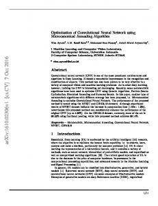
Figure 2. Remeshing. (a) A triangular mesh is morphed into a pseudo cube (b) aligned with its principal axes by iteratively applying volumetric deformations (Gregson et al., 2011). A semi-regular quad-mesh (c) is then defined on the pseudo-cube and we project its vertices onto the original mesh to create the regular tesselation of the original shape shown in (d).

on a GPU, forcing the use of the CPU, which is much slower. In theory, this could be remedied by storing the exponential terms of Eq. 3 in adjacency matrices, as by Monti et al. (2016). However, densely representing those matrices, would not be practical because it would be too large to fit on the GPU for real-world problems. A sparse representation would solve the memory problem but would be equally impractical because, unlike by Monti et al. (2016), the geodesic distances change at every iteration and have to be recomputed. Filling these new values into a sparse representation that fits on the GPU would also be very slow.

Cube-Mesh mapping. To overcome this difficulty, we propose to exploit the properties of cube and poly-cube maps (Tarini et al., 2004), which allow the remeshing of 3D shapes homotopic to spheres such as those of cars or bicycles shells as semi-regular quad-meshes with few irregular vertices, a uniform tessellation density and well-shaped quads (Bommes et al., 2013). Fig. 2 illustrates this process. After remeshing, we can perform the convolutions of Eqs. 3 and 4 for all regular vertices using GPU acceleration. However, a few irregular vertices are unavoidable for most shapes, according to index theory (Bommes et al., 2012). We handle them as special cases, at the cost of a small approximation described in the supplementary material. In practice, we have in memory one “image” per face of the bottom-right box of Fig. 2, and each pixel of the said images has three channels corresponding to the 3d coordinates of that point in the remeshed shape, which is used to compute the values of ρ() and θ(), which can now be done in a GPU-friendly manner.

Interestingly, as shown in the experiments, we noticed that by learning to predict more physical quantities than actually needed, through additional branches, as by Caruana (1997); Ramsundar et al. (2015) we favour the emergence intermediate-level features that are more robust and less overfitting prone. This observation hints that our architecture is actually learning physical phenomenons and not only interpolating the output. As discussed above, all these operations could be implemented using geodesic nets that operate directly on M and perform convolutions such as those of Eq. 3, but this would be slow. In practice, we first map a reference shape on a cube such as the one depicted at the bottom right of Fig. 2 to obtain a semi-regular quad-remeshing. Then, X becomes the set of 3D coordinates assigned to each vertex of the resulting regular vertex grid, which we then use to reconstruct either identical or modified versions of the 3D shape, such as the one shown at the bottom left of Fig. 2. To increase the receptive field of our convolutions without needlessly increasing the number of parameters or reducing the resolution of our input, we use dilated convolutions (Yu & Koltun, 2016), along with several convolutional blocks with pass-through residual connections (He et al., 2016).

4. Shape Optimization Once trained, the regressor Fω can be used as a surrogate model or proxy to evaluate the effectiveness of a particular design. Not only is it fast, but it is also differentiable with respect to the X coordinates that control the shape. We can therefore use a gradient-based technique to maximize the desirable property while enforcing design constraints, such as the fact that a bicycle shell must be wide enough to accommodate the rider, a car must contain a pre-defined volume for the engine and passengers, or a plane wing should be thick enough to have the required structural rigidity. Formally, this can be expressed by treating Fω as a function

Geodesic Convolutional Shape Optimization

Fωy

{

X

Fωz

Fω0 Atrous geo conv

Atrous geo conv block

Residual connection

Mean pooling

Fully connected layer

Figure 3. The architecture of our geometric CNN. The vertex coordinates of the quad-mesh of Fig. 2 are fed to a convnet that produces a feature map, which is itself fed to both another convnet and a fully connected one. The first outputs a vector of pressure values and the second a scalar drag value. Using the same features for both prevents overfitting.

of X and looking for X∗ = argmin G (Fω (X)) s.t C(X) ≤ 0,

(5)

X

where G is a fitness function, such as the negative Lift-toDrag ratio in the case of a wing or simply the drag in the case of the car, and C represents the set of constraints that a shape must satisfy to be feasible. 4.1. Projected Gradient Descent To solve the minization problem of Eq. 5, we use a projected version of the popular ADAM algorithm (Kingma & Ba, 2015): at the end of each iteration, we check if the X still is a feasible shape. If not, we project it to closest feasible point. To do this effectively, we need to compute the Jacobians ∇X G (Fω (X)) and ∇X C(X),

(6)

which we do using the standard chain rule through automatic differentiation. Fig. 4 depicts such a minimization. −∇X G

−∇X G

these parameters X(C) and reformulate the minimization problem of Eq. 5 as a minimization with respect to C. For example, wings have long been described in terms of their NACA-4digits parameters (Jacobs et al., 1948), which are three real numbers representing a family of shapes known to have good aerodynamic properties. These numbers correspond to the maximum camber, its location, and the wing thickness. By contrast to Kriging, the performance of our approach increases with the number of parameters, which we will demonstrate in the result section by using 18 parameters instead of only the 3 NACA ones for airfoil profiles. To further increase flexibility, we could replace the parametric models by the Laplacian parameterization introduced by Ngo et al. (2016), as demonstrated in the 2D case in the supplementary material. It expresses all vertex coordinates as linear combinations of those of a small number of control vertices. Thus, the objective function will become a differentiable function of the positions of a subset of mesh vertices. Our approach will therefore directly apply, which would let us adjust the model’s complexity as needed by adding or removing control points. 4.3. Online Learning

Figure 4. Minimizing the drag of the initially spherical surface under the constraint it must contain the smaller red sphere.

4.2. Parametrization Given the size of the meshes we deal with, the optimization problem of Eq. 5 is a very large one, which traditional methods such as Kriging (Toal & Keane, 2011; Xu et al., 2017) cannot handle. To reduce the problem’s dimensionality and make comparisons possible, we introduce parametric models. More specifically, when the shape and its pose are controlled by a small number of parameters C, we can write the vertex coordinates as a differentiable function of

We start from of an initial set of random shapes on which we run a full simulation to generate the triplets (Mi , Yi , Zi ). We then use it to train Fω by minimizing the loss of Eq. 1. If the database used to train the network is not representative enough, X can drift away from regions of the shape space where our proxy provides a good approximation. Since performing even a single simulation is much slower than running many ADAM optimization steps, we alternate between the following two-steps. 1. We run project gradient steps as discussed above using the current Fω GCNN regressor until convergence.

Geodesic Convolutional Shape Optimization

2. We run a new simulation for the obtained shape, add this new sample to the training set and fine tune the Fω GCNN regressor with this new training sample.

Fz = 3.223, Z = 3.237

Fz = 0.719, Z = 0.710

Note that in an industrial setting, the randomly chosen set of initial samples could be replaced by all the shapes that have been simulated in the past. Over time, this would result in an increasingly competent proxy that would require less and less re-training.

Fz = 0.245, Z = 0.244

Fz = 3.094, Z = 3.038

5. Experimental Results In this section, we evaluate our proposed shape optimization pipeline. It is designed to handle 3D shapes but can also handle 2D ones by simply considering the 2D equivalent of a surface mesh, which is a discretized 2D contour. We therefore first present results on 2D airfoil profiles, which have become a de facto standard in the CFD community for benchmarking shape optimization algorithms (Toal & Keane, 2011; Orman & Durmus, 2016). We then use the example of car shapes to evaluate our algorithm’s behavior in the more challenging 3D case. We implemented our deeplearning algorithms in TensorFlow (Abadi et al., 2016) and ran them on a single Titan X Pascal GPU. We will quantify the accuracy of various regressors in terms of the standard L2 mean percentage error over a test set Sv , that is, yn k2 n −ˆ Ay = 1.0 − En∈Sv [ kyky ], (7) n k2 where y denotes either a ground truth local quantity Yi or the global one Zi . In turn, yˆ denotes the corresponding predictions F y (Xi ) or F z (Xi ). 5.1. 2D Shapes - Airfoils and Hydrofoils Training and testing data. As discussed above, airfoil profiles have long been parameterized using three NACA parameters (Jacobs et al., 1948). To generate our training and validation data, we create 8000 training and 8000 testing shapes, such as those depicted by the blue outlines at the top of Fig. 5. To this end, we randomly select NACA parameters and then further randomize the shape. This is intended to demonstrate that our approach remains effective even when the training shapes belong to a much larger set of shapes that can be far from desirable. We use the popular CFD simulator XFoil to compute their aerodynamic properties. It takes as input a discretized outline, solves the flow problem using an inviscid-vorticity panel method, and applies a compressibility correction (Drela, 1989). We will demonstrate below that our regressor learned from such non-aerodynamic shapes can nevertheless be used to refine a profile and obtain truly efficient ones, such as those shown at the bottom of Fig. 5. GCNN design choices. We tested several architectures to implement the regressor Fω of Eq. 1.

Initialization, G = 98.47

Ours-NACA, G = −1.23

Ours-18DOF, G = −1.26

GP-NACA, G = −1.15

GP-18DOF, G = −1.10

Figure 5. 2D Profiles. (Top) Pressure and drag estimates on four profiles from the testing set, shown in blue. The red and green solid lines depict the ground-truth pressure values above and below. Z is the ground-truth drag. The red and green crosses depict the predicted pressure values, which mostly fall on the corresponding curves. Fz is the predicted drag, which is also close to Z. (Bottom) Starting from the shape on the left, we obtain the shapes in the middle using the standard NACA 3-parameter deformation model and the shapes on the right using the more complex 18-parameter model. In both cases, we obtain a lower value of the objective function G using our regressor than the GP ones.

Model Standard Separate Dilated Separate Joint 2 Branches Joint 4 Branches

ACp 0.6877 0.7442 0.8132 0.8203

ACD 0.8223 0.8406 0.8490 0.8601

Figure 6. Prediction accuracy for the pressure profile along the airfoil Cp ∈ RN and the drag coefficient CD ∈ R on 8000 randomly generated airfoil shapes.

• Standard Separate: We use two separate GCNN architectures for drag and pressure prediction. They are exactly the same as discussed in Section 3.2, except that only one of the final branches is created for each and we use dense 3 × 3 convolutional filters instead of dilated ones. • Dilated Separate: We replace the usual convolutions by dilated ones, which include a spacing between kernel values (Yu & Koltun, 2016). • Joint 2 Branches: We replace the two separate networks by a shared common branch F0 followed by separate branches F y and F z for drag and pressure, as discussed in Section 3.2. • Joint 4 Branches: We push the idea of using separate branches connected to a shared one a step further by adding two more branches that predict the skin friction coefficient along the airfoil and edge fluid

Geodesic Convolutional Shape Optimization

velocity. Although these quantities are not used to compute the objective function, the hope is that forcing the network to predict them helps the joint branch to learn the right features. This is known as disentangling in the Computer Vision literature and has been observed to boost performance (Caruana, 1997; Rifai et al., 2012; Ramsundar et al., 2015). We report the accuracy results for these four architectures in Table 6. As observed by Chen et al. (2015) for dense semantic image segmentation, the dilated convolutions perform better than the standard ones for regression of dense outputs. Both joint architectures do better than the separate ones, with disentangling providing a further performance boost. At the top of Fig. 5, we superpose the pressure vector computed using the simulator and those predicted by the Joint 4 Branches architecture for 4 different profiles. Comparing to standard regressors. Since our Joint 4 Branches GCNN architecture performs best, we will refer to it as Ours and we now compare its accuracy to that of two standard regressors, one based on Gaussian Processes (GPs) and the other on K-Nearest Neighbours (KNNs). For GPs, we use squared exponential kernels because they have recently be shown to be effective for aerodynamic prediction tasks (Toal & Keane, 2011; Rosenbaum & Schulz, 2013; Chiplunkar et al., 2017). For KNN regression, we empirically determined that K = 8 combined to a distance-based neighbor weighting yielded the best results. Note that in order to compare to such parametric methods, in this experiment only, we restrict our training and test set to the NACA parameter space. The three curves at the top of Fig. 7 represent the mean accuracy of the predicted drag and its variance as function of the number of samples used to train the regressors. Our approach consistently outperforms the other two, especially when there are few training samples. One possible interpretation is that, because our regressor operates directly on the shape of the object unlike the other two regress from the NACA parameters, it learns the local physical interactions between discretization vertices and can therefore generalize well to unseen shapes. Shape optimization. We now use our regressor along with the baseline ones to maximize lift while keeping drag constant. To this end, we take the fitness function of Eq. 5 to be G(Y, Z) = −CL (Y) + λ(Z − Ztarget )2 , where CL is the function that integrates the pressure values Y to estimate the lift, Ztarget is the drag target, and λ is a parameter that controls the relative importance of the two terms. In our experiments, we set λ = 100 and Ztarget = 0.8. In the bottom graph of Fig. 7, we show the resulting lift values after performing shape optimization, again as a function of the number of training samples used to train the regressor.

0.8

ACD 0.6

GP K-NN Ours

0.4 0.2 1.2 1.0

−G

0.8

GP online Ours offline Ours online

0.6 102

103 training set size Figure 7. Comparative results for 2D airfoils.(Top) Accuracy of drag prediction. (Bottom) Shape optimization.

The resulting wing profiles are shown at the bottom middle of Fig. 5. We also plot the corresponding results of a standard GPbased method, also known as kriging (Jeong et al., 2005; Toal & Keane, 2011; Nardari et al., 2017; Xu et al., 2017), an industry standard as discussed in Section 2.1. Kriging can also be used either offline or online, that is without or with retraining the regressor during the optimization process. To implement the retraining, we relied on an optimal tradeoff strategy between exploitation and exploration (Toal & Keane, 2011). Note that our regressor is good enough to outperform GP online even without retraining. In a last experiment, we reparameterized the wing shape in terms of 19 parameters instead of the usual 3 from NACA, as described in detail in the supplementary material. We performed the computation again using this new parameter set in conjunction with either our approach or GPs. The results are shown at the bottom right of Fig. 5 and demonstrate our approach’s ability to deal with larger models. 5.2. 3D Shapes - Cars Training and Testing Data. datasets

We use the four following

• SYNT-TRAIN : It is a dataset of 2000 randomly generated 3D shapes such as the one shown at the top of Fig. 1, which does not need to be car-like. • SYNT-TEST: 50 more random shapes generated in the same way as those of SYNT-TRAIN for testing purposes. • CARS-FineTune : We downloaded 6 cars CAD models from the web. Two of them are kept for finetuning. We augment each model with 3 scaling factors and 9 rotations, to obtain a total of 54 cars. • CARS-TEST : The four remaining CAD models held

Geodesic Convolutional Shape Optimization

out for final testing, yielding a total of 108 shapes after augmentation. To generate our random shapes, we introduce a function fC : R3 → R3 , where C represents the parameters that control its behavior and apply it to an initially spherical set of vertices X0 . f is an algebraic function that applies rotations, translations, affine transformations, and dilatations with respect to the center of the shape, which lets us create a wide variety of shapes. The shape at the top Fig. 1 is one of them and we provide more in the supplementary material. We give the precise definition of f in the supplementary material and take C to be a 21D vector. We used the industry standard Ansys Fluent (Inc., 2011) to compute their aerodynamic properties with the k-epsilon turbulence model. Method CNN Ours

VALID ACD 70.1 % 77.2%

TEST ACD 38.4% 51.5 %

TEST-FT ACD 58.1% 70.3%

Figure 8. Regression results on our three 3D test sets.

Comparing to Standard Regressors. In Fig. 8, we report the accuracy of our regressor under three different training and testing scenarios: • VALID : The regressor is first trained on SYNT-TRAIN and tested on SYNT-TEST. This is a sanity check since testing is carried out on shapes that have the same statistical distribution as the training ones. • TEST : The regressor is trained on SYNT-TRAIN and tested on CARS-TEST. This is much more challenging since the testing shapes are those of real cars while the training ones are not. • TEST-FT : The regressor is trained on SYNT-TRAIN, fine tuned using CARS-FineTune, and tested on CARS-TEST. This is similar to TEST but we help the regressor by giving it a few real car shapes making a few additional epochs of training. Unsurprisingly, the accuracy on TEST is lower than on VALID. Nevertheless, fine-tuning with a few car-like examples brings it back up. To assess the importance of using GCNNs instead of regular CNNs, we re-ran all three scenarios using a standard CNN of similar complexity. In other terms, we keep the same architecture where the geodesic convolutions of Eqs. 3 and 4, are replaced by standard ones. As can be seen on the top row of the figure, the accuracy numbers are much worse in all three cases. Shape Optimization In this section, we use the GCNN regressor pre-trained on our SYNT-TRAIN data to minimize the drag generated by a car-like shape, that is, G(Y, Z) = Z.

Method Ours - Online Ours - OffLine GP - Online

Init 80.2 80.2 80.2

50 Sim 4.91 7.56 16.65

100 Sim 4.71 7.56 12.56

Figure 9. 3D car shape optimization. (Top) Feasible shapes must remain out of the two parallelepipeds. (Bottom) Drag of the optimized shapes given the number of calls to the simulator for the online methods.

Without constraints, the shape would collapse to an infinitely thin one. To allows for passengers and an engine, we need the constraint C of Eq. 5. Feasible shapes are defined as those that remain outside of two parallelepiped, one for the engine and the other for the passenger compartment, as shown at the top of Fig. 9. As in the case of the airfoils, the GP regressor takes as input the 21 parameters C of the deformation function fC introduced above while ours operates directly on the surface mesh. The initial shape X0 that fC operates on is the CAD model of a car shown on the left at bottom of Fig. 1 and the result is shown on the right. At the bottom of Fig. 9, we report the resulting drag for a given number of call to the simulator during the minimization, 50 or 100 for the online methods and 0 for the offline one. Again whether offline or online, our approach outperforms the online version of GP and finds a better optimum for the 21 parameters. In the online case, note that with only 50 calls to the simulator our result is already close to the optimum even though our network, pre-trained on SYNT-TRAIN, had never seen a car before.

6. Conclusion We have shown that we could first train Geodesic CNNs to reliably emulate a output of a CFD simulator and then use them to optimize them the aerodynamic performance of a shape. As a result, we can outperform state-of-the-art techniques by 5 to 20% on relatively simple 2D problems and solve previously unsolvable ones. In our current implementation, we use parameterized models to reduce the shape’s number of degrees of freedom and make the optimization problem tractable. Since our method can operate on generic meshes, in future work, we intend This work was realized with the help of the software ANSYS by ANSYS Inc.

Geodesic Convolutional Shape Optimization

to use the Laplacian parameterization introduced by Ngo et al. (2016) to increase or decrease the number of degrees of freedom at will and make our approach fully flexible.

Drela, M. XFOIL: An Analysis and Design System for Low Reynolds Number Airfoils. In Conference on Low Reynolds Number Aerodynamics, pp. 1–12, Berlin, Heidelberg, 1989. Springer Berlin Heidelberg.

References

Gao, Yisheng, Wu, Yizhao, and Xia, Jian. Automatic Differentiation Dased Discrete Adjoint Method for Aerodynamic Design Optimization on Unstructured Meshes. Chinese Journal of Aeronautics, 30(2):611 – 627, 2017.

Abadi, Mart´ın, Barham, Paul, Chen, Jianmin, Chen, Zhifeng, Davis, Andy, Dean, Jeffrey, Devin, Matthieu, Ghemawat, Sanjay, Irving, Geoffrey, Isard, Michael, Kudlur, Manjunath, Levenberg, Josh, Monga, Rajat, Moore, Sherry, Murray, Derek G., Steiner, Benoit, Tucker, Paul, Vasudevan, Vijay, Warden, Pete, Wicke, Martin, Yu, Yuan, and Zheng, Xiaoqiang. Tensorflow: A system for large-scale machine learning. In USENIX Conference on Operating Systems Design and Implementation, pp. 265–283, 2016. Alexandersen, J., Sigmund, O., and Aage, N. Large Scale Three-Dimensional Topology Optimization of Heat Sinks Cooled by Natural Convection. International Journal of Heat and Mass Transfer, 100(Supplement C):876 – 891, 2016. ISSN 0017-9310. Allaire, G. A Review of Adjoint Methods for Sensitivity Analysis, Uncertainty Quantification and Optimization in Numerical Codes. Ing´enieurs de l’Automobile, 836: 33–36, July 2015. Bengio, Y., Delalleau, O., and Roux, N. Le. The Curse of Highly Variable Functions for Local Kernel Machines. In Advances in Neural Information Processing Systems, pp. 107–114, 2006. Bommes, D., Lvy, B., Pietroni, N., Puppo, E., a, C. Silv, Tarini, M., and Zorin, D. State of the art in quad meshing. In Eurographics STARS, 2012. Bommes, David, L´evy, Bruno, Pietroni, Nico, Puppo, Enrico, Silva, Claudio, Tarini, Marco, and Zorin, Denis. Quad-mesh generation and processing: A survey. Comput. Graph. Forum, 32(6):51–76, September 2013. ISSN 0167-7055. doi: 10.1111/cgf.12014.

Gholizadeh, S. and Seyedpoor, S.M. Shape Optimization of Arch Dams by Metaheuristics and Neural Networks for Frequency Constraints . Scientia Iranica, 18(5):1020 – 1027, 2011. Gosselin, L., Tye-Gingras, M., and Mathieu-Potvin, F. Review of Utilization of Genetic Algorithms in Heat Transfer Problems. International Journal of Heat and Mass Transfer, 52(9):2169 – 2188, 2009. Gregson, James, Sheffer, Alla, and Zhang, Eugene. All-hex mesh generation via volumetric polycube deformation. In Computer graphics forum, volume 30, pp. 1407–1416. Wiley Online Library, 2011. Guo, X., Li, W., and Iorio, F. Convolutional Neural Networks for Steady Flow Approximation. In Conference on Knowledge Discovery and Data Mining, 2016. He, K., Zhang, X., Ren, S., and Sun, J. Deep residual learning for image recognition. In Conference on Computer Vision and Pattern Recognition, pp. 770–778, 2016. Inc., Ansys. ANSYS FLUENT Theory Guide. November 2011. Jacobs, Eastmann N., Ward, Kenneth E., and Pinkerton, Robert M. The characteristics of 78 related airfoil sections from tests in the variable density wind tunnel. Technical Report 460, 1948. Jeong, Shinkyu, Murayama, Mitsuhiro, and Yamamoto, Kazuomi. Efficient optimization design method using kriging model. Journal of Aircraft, 42(2):413–420, 2005.

Caruana, R. Multitask Learning. Machine Learning, 28, 1997.

Kingma, D.P. and Ba, J. Adam: A Method for Stochastic Optimisation. In International Conference for Learning Representations, 2015.

Chen, L.-C., Papandreou, G., Kokkinos, I., Murphy, K., and Yuille, A. Semantic Image Segmentation with Deep Convolutional Nets and Fully Connected CRFs. In International Conference for Learning Representations, 2015.

Kipf, Thomas N and Welling, Max. Semi-supervised classification with graph convolutional networks. arXiv preprint arXiv:1609.02907, 2016.

Chiplunkar, Ankit, Bosco, Elisa, and Morlier, Joseph. Gaussian process for aerodynamic pressures prediction in fast fluid structure interaction simulations. In World Congress of Structural and Multidisciplinary Optimisation, pp. 221– 233. Springer, 2017.

Lundberg, A., Hamlin, P., Shankar, D., Broniewicz, A., Walker, T., and Landstram, C. Automated Aerodynamic Vehicle Shape Optimization Using Neural Networks and Evolutionary Optimization. SAE International Journal of Passenger Cars - Mechanical Systems, 8:242–251, April 2015.

Geodesic Convolutional Shape Optimization

McNamara, G. and Zanetti, G. Use of the Boltzmann Equation to Simulate Lattice-gas Automata. Physical Review Letters, 61(20):2332, 1988.

Tarini, M., Hormann, K., Cignoni, P., and Montani, C. Polycube-maps. ACM Transactions on Graphics, 23(3): 853–860, 2004.

Monti, Federico, Boscaini, Davide, Masci, Jonathan, Rodol`a, Emanuele, Svoboda, Jan, and Bronstein, Michael M. Geometric deep learning on graphs and manifolds using mixture model cnns. arXiv preprint arXiv:1611.08402, 2016.

Toal, David JJ and Keane, Andy J. Efficient multipoint aerodynamic design optimization via cokriging. Journal of Aircraft, 48(5):1685–1695, 2011.

Nardari, C., Mann, A., and Schindele, T. Characterization of the effects of manufacturing geometry details on exhaust flow noise using lattice boltzmann based method simulations. 2017. Ngo, D., Ostlund, J., and Fua, P. Template-Based Monocular 3D Shape Recovery Using Laplacian Meshes. IEEE Transactions on Pattern Analysis and Machine Intelligence, 38(1):172–187, 2016. Orman, E. and Durmus, G. Comparison of Shape Optimization Techniques Coupled with Genetic Algorithms for a Wind Turbine Airfoil. In IEEE Aerospace Conference, pp. 1–7, March 2016.

Tompson, J., Schlachter, K., Sprechmann, P., and Perlin, K. Accelerating Eulerian Fluid Simulation With Convolutional Networks. ArXiv e-prints, July 2016. Ulaganathan, S. and Asproulis, N. Surrogate Models for Aerodynamic Shape Optimization, pp. 285–312. Springer, 2013. Xian, W. and Takayuki, A. Multi-GPU Performance of Incompressible Flow Computation by Lattice Boltzmann Method on GPU Cluster. Parallel Computing, 37(9): 521–535, 2011. Xu, Gang, Liang, Xifeng, Yao, Shuanbao, Chen, Dawei, and Li, Zhiwei. Multi-objective aerodynamic optimization of the streamlined shape of high-speed trains based on the kriging model. PLOS ONE, 12(1):1–14, 01 2017.

Preen, R. J. and Bull, L. Toward the Coevolution of Novel Vertical-Axis Wind Turbines. IEEE Transactions on Evolutionary Computation, 2:284–293, 2015.

Yu, F. and Koltun, V. Multi-Scale Context Aggregation by Dilated Convolutions. In ICLR, 2016.

Quarteroni, A. and Quarteroni, S. Numerical Models for Differential Problems, volume 2. Springer, 2009.

7. Appendix

Ramsundar, Bharath, Kearnes, Steven M., Riley, Patrick, Webster, Dale, Konerding, David E., and Pande, Vijay S. Massively multitask networks for drug discovery. CoRR, abs/1502.02072, 2015.

In this supplementary material, we first provide additional detail on the handling of the irregular vertices of the CubeMesh CNNs of Section 3.1. We then give analytical definitions of the 2D and 3D deformation parameterizations of Sections 5.1 and 5.2.

Rasmussen, C. E. and Williams, C. K. Gaussian Process for Machine Learning. MIT Press, 2006. Rifai, Salah, Bengio, Yoshua, Courville, Aaron, Vincent, Pascal, and Mirza, Mehdi. Disentangling factors of variation for facial expression recognition. In Fitzgibbon, Andrew, Lazebnik, Svetlana, Perona, Pietro, Sato, Yoichi, and Schmid, Cordelia (eds.), Computer Vision – ECCV 2012, pp. 808–822, Berlin, Heidelberg, 2012. Springer Berlin Heidelberg. Rosenbaum, Benjamin and Schulz, Volker. Response surface methods for efficient aerodynamic surrogate models. In Computational Flight Testing, pp. 113–129. Springer, 2013. Skinner, S.N. and Zare-Behtash, H. State-of-the-art in aerodynamic shape optimisation methods. Applied Soft Computing, 62(Supplement C):933 – 962, 2018. ISSN 15684946.

7.1. Handling Singular Points for Semi-Regular Quad-Meshes As discussed in Section 3.1 of the paper, when mapping a surface onto a cube-mesh, we have to deal with irregular vertices, which correspond to the corners of the cube and have three neighbors instead of four. To perform convolutions efficiently we first unfold the cube surface onto a plane. As illustrated by Fig. 10, we can then simply pad irregular corners with the feature values associated to cube edges. This enables us to use standard convolutional kernels even in the neighborhood of irregular vertices. Furthermore, since we use Geodesic Convolutions, the irregularity is naturally handled by the interpolation operation. 7.2. Airfoil Parameterization in 2D In this section we will first briefly describe the standard NACA airfoil 4 digit parameterization (Jacobs et al., 1948),

Geodesic Convolutional Shape Optimization

18-parameter foils. We increase the number of degrees of freedom by that writing the 3 parameters t, m, p as quadratic functions of x, that is, Diagonal Expansion

t(x) = t0 + t1 x + t2 x2 m(x) = m0 + m1 x + m2 x2 p(x) = p0 + p1 x + p2 x2 Convolutional filter. Dilation Factor = 1

Features on the diagonal.

Convolutional filter. Dilation Factor = 2 Cube-Mapped Quad-Mesh

Figure 10. Handling the singularities of the Quad-Mesh for convolution purposes.

which, confusingly involves 3 degrees of freedom. We then discussed our extension to 19 degrees of freedom. NACA 4 digit. Without loss of generality, we can assume that the airfoil is of unitary cord length and let 0 ≤ x ≤ 1 the coordinate that defines the position along that length. Let us further consider the airfoil thickness t, maximum camber m , along with its location p. To compute the airfoil shape, we first define the mean camber line  m
2px − x2 ,   2  p

yc =

  

0≤x≤p


m (1 − 2p) + 2px − x2 , 2 (1 − p)

p≤x≤1

and the airfoil thickness to camber yt as   √ 5t 0.2969 x − 0.1260x − 0.3516x2 + 0.2843x3 − 0.1015x4 .

Since the thickness needs to be applied perpendicular to the camber line, the coordinates (xU , yU ) and (xL , yL ), of the upper and lower airfoil surface, respectively, become xU = x − yt sin θ, xL = x + yt sin θ,

yU = yc + yt cos θ,

(8)

yL = yc − yt cos θ,

(9)

where 

 dyc , dx

θ = arctan  2m  0≤x≤p  2 (p − x),   p dyc =  dx  2m   (p − x), p ≤ x ≤ 1 (1 − p)2

(10)

(11)

Thus, the wing shape is entirely defined by the choice of t, m , and p.

where the the pi , mi , and qi control the new degrees of freedom. Moreover we allow the lower and upper airfoil surfaces to be associated two two different camber lines, hence doubling the total number of degrees of freedom to 2 × (3 + 3 + 3). 7.3. Surface Parameterization in 3D As discussed in Section 5.2, we parametrize 3D shape deformations using a transformation function fC : R3 → R3 that applies to the vertices of an initial shape X0 , where C is a 21D vector. For clarity, let us split the 21 components of C into three groups, one for each axis C = {Cix }i=0...6 ∪ {Ciy }i=0...6 ∪ {Ciz }i=0...6 . As show in Fig. 9, Lx , Ly , Lz , denote the maximal size over each dimension and let (x, y, z) be the coordinates of a specific vertex X. We write fC (X)x = C0x + x[C1x + C2x x y z + C3x cos( 2π) + C4x cos( 2π) Ly Lz y z + C5x sin( 2π) + C6x sin( 2π)] , Ly Lz fC (X)y = C0y + y[C1x + C2y y x x + C3y cos( π) + C4y cos( 2π) Lx Lx x x y y + C5 sin( π) + C6 sin( 2π)] , Lx Lx fC (X)z = C0z + z[C1x + C2z z x x + C3z cos( π) + C4z cos( 2π) Lx Lx x x + C5z sin( π) + C6z sin( 2π)] . Lx Lx This simple parametric transformation provides enough freedom to generate sophisticated shapes. Furthermore, the initial shape corresponds to setting all the parameters to 0, except from C1x , C1y , C1z , which are set to 1.