MASTER OF SCIENCE in the Department of Computer Science. @ Jeffrey Christopher Hornsberger, 2004. University of Victoria. All rights resewed. This thesis ...
Geographic Grid Routing for Wireless Sensor Networks by Jeffrey Christopher Hornsberger B.Sc., University of Victoria, 2002
A Thesis Submitted in Partial Fulfillment of the Requirements for the Degree of
MASTEROF SCIENCE in the Department of Computer Science
@ Jeffrey Christopher Hornsberger, 2004 University of Victoria All rights resewed. This thesis may not be reproduced in whole or in part by photocopy or other means, without the permission of the author
Supervisor: Dr. G.C. Shoja
ABSTRACT High resolution data coIIection using low-cost wireless sensor networks has recently become feasible due to advances in electronics and wireless networking technologies. Unique factors such as large network size, particular traffic patterns and severe power limitations necessitate targeted research in the area of sensor network routing. Geographic Grid Routing (GGR) is described in detail in this thesis. GGR aims to provide robust task dissemination and data collection from large sensor networks using geographic routing to reduce stored state information and used energy. In this way the useful lifetime of the network is prolonged. The work builds on a previously developed routing protocol called Two-Tier Data Dissemination (TTDD). Our work is differentiated by the use of multiple paths, a more efficient and realistic data collection model, and more realistic environmental assumptions. Realistic experiments are used to evaluate the performance of GGR. This thesis investigates the correctness, performance and applicability of the GGR protocol. The protocol is validated using state-of-the-art model checking software and the advantages of GGR over TTDD are shown through mathematical modeling. The GGR protocol is implemented using the latest network simulation software with our own extensions that result in a realistic sensor network model. Performance tests were conducted at the University of Victoria's Research Computing Facility. The results show GGR to be a highly scalable, versatile and robust solution.
Table of Contents
Abstract
ii
Table of Contents
iv
List of Tables
viii
List of Figures
ix
List of Abbreviations
xii
Acknowledgement
xiii
1 Introduction
1
1.3
............................... Description . . . . . . . . . . . . . . . . . . . . . . . . . . . . . . . . . . Current Research . . . . . . . . . . . , . . . . . . . . . . . . . . . . . . .
4
1.4
Outline
. . .. . .. .. .. .- .. ... . ... .. .... . . ... ...
5
1.1 1.2
Motivation . . .
2.2 2.3
2
6
2 Background 2.1
1
.................... Routing in Sensor Networks . . . . . . . . . . . . . . . . . . . . . . . . . Previous Work . . . . . . . . . . . . . . . . . - . . . . . . . . . . . . . .
Routing in Ad Hoc Networks
.. . .
8
9 13
2.3.3
. . . . . . . . . . . . - . . . . - . . . . . . . . . . 13 Gossiping . . . . . . . . . . . . . . . . . . . . . . . . . . . . . . 14 Small Minimum-Energy Communication Network . . . . . . . . . 15
2.3.4
Sensor Protocols for Information via Negotiation
2.3.1 2.3.2
Flooding . . .
. . . . . . . . . . 15
Table of Contents
v
2.3.5
Sequential Assignment Routing . . . . . . . . . . . . . . . . . . . 16
2.3.6
Low-Energy Adaptive Clustering Hierarchy . . . . . . . . . . . . 17
2.3.7
Directed Diffusion . . . . . . . . . . . . . . . . . . . . . . . . . . 18
2.3.8
Geographical and Energy Aware Routing . . . . . . . . . . . . . . 19
2.3.9
GRAdient Broadcast . . . . . . . . . . . . . . . . . . . . . . . . . 20
2.3.10 Two-Tier Data Dissemination . . . . . . . . . . . . . . . . . . . . 21 2.4
Advancing the Current State of the Art . . . . . . . . . . . . . . . . . . . 23
3 Problem Statement. Proposed Solution and Methodology 3.1
3.2
Problem Definition . . . . . . . . . . . . . . . . . . . . . . . . . . . . . . 26 3.1.1
Scope and Assumptions . . . . . . . . . . . . . . . . . . . . . . . 26
3.1.2
Statement of the Problem . . . . . . . . . . . . . . . . . . . . . . 27
Solution Overview . . . . . . . . . . . . . . . . . . . . . . . . . . . . . . 28 3.2.1
3.3
25
Qualitative Analysis and Comparison . . . . . . . . . . . . . . . . 29
Methodology . . . . . . . . . . . . . . . . . . . . . . . . . . . . . . . . .
31
3.3.1
Formal Verification and Analysis . . . . . . . . . . . . . . . . . . 32
3.3.2
Performance Evaluation . . . . . . . . . . . . . . . . . . . . . . . 33
4 Protocol Design
34
4.1
Sequence Number Usage . . . . . . . . . . . . . . . . . . . . . . . . . . . 36
4.2
Link Sublayer Operation . . . . . . . . . . . . . . . . . . . . . . . . . . . 37
4.3
Grid Construction . . . . . . . . . . . . . . . . . . . . . . . . . . . . . .
38
4.4
Sink Operation . . . . . . . . . . . . . . . . . . . . . . . . . . . . . . . .
39
4.4.1
Task Assignment . . . . . . . . . . . . . . . . . . . . . . . . . . .
39
4.4.2
Event-Driven Grid Reconstruction . . . . . . . . . . . . . . . . . 41
4.5
Intermediate Node Operation . . . . . . . . . . . . . . . . . . . . . . . . 42
4.6
Dissemination Node Operation . . . . . . . . . . . . . . . . . . . . . . . . 43 4.6.1 4.6.2
. . . . . . . . . . . . . 44 Data Forwarding . . . . . . . . . . . . . . . . . . . . . . . . . . . 48
Task Dissemination and Role Assignment
Table of Contents 4.7
Task Dissemination Within the Region of Interest . . . . . . . . . . . . . . 51
4.8
Sensing Node Operation . . . . . . . . . . . . . . . . . . . . . . . . . . . 55
4.9
Configuration Parameters . . . . . . . . . . . . . . . . . . . . . . . . . . 55
59
5 Analysis 5.1
5.2
Protocol Verification . . . . . . . . . . . . . . . . . . . . . . . . . . . . . 59 5.1.1
Overview of SPIN . . . . . . . . . . . . . . . . . . . . . . . . . . 59
5.1.2
GGRModel . . . . . . . . . . . . . . . . . . . . . . . . . . . . . 60
Overhead Analysis . . . . . . . . . . . . . . . . . . . . . . . . . . . . . . 62 5.2.1
Model and Notations . . . . . . . . . . . . . . . . . . . . . . . . . 62
5.2.2
Communication Overhead . . . . . . . . . . . . . . . . . . . . . . 64
5.2.3
State Complexity . . . . . . . . . . . . . . . . . . . . . . . . . . . 67
6 Prototyping and Simulation 6.1
6.2
7
vi
72
Simulation Environment . . . . . . . . . . . . . . . . . . . . . . . . . . . 72 6.1.1
Selection . . . . . . . . . . . . . . . . . . . . . . . . . . . . . . . 72
6.1.2
Operation . . . . . . . . . . . . . . . . . . . . . . . . . . . . . . . 73
Implementation Design . . . . . . . . . . . . . . . . . . . . . . . . . . . . 75 6.2.1
Energy Model . . . . . . . . . . . . . . . . . . . . . . . . . . . . 76
6.2.2
Failure Model . . . . . . . . . . . . . . . . . . . . . . . . . . . . 77
6.2.3
Applications . . . . . . . . . . . . . . . . . . . . . . . . . . . . . 77
Performance Evaluation
79
7.1
Evaluation Scenarios . . . . . . . . . . . . . . . . . . . . . . . . . . . . . 79
7.2
Performance Metrics . . . . . . . . . . . . . . . . . . . . . . . . . . . . .
81
7.3
Results . . . . . . . . . . . . . . . . . . . . . . . . . . . . . . . . . . . .
81
7.3.1
Delivery Efficiency . . . . . . . . . . . . . . . . . . . . . . . . .
81
7.3.2
Delay . . . . . . . . . . . . . . . . . . . . . . . . . . . . . . . . . 85
7.3.3
Energy Efficiency . . . . . . . . . . . . . . . . . . . . . . . . . . 86
Table of Contents 7.4
vii
Comparison to TTDD . . . . . . . . . . . . . . . . . . . . . . . . . . . . 90
8 Conclusions
91
8.1
Summary . . . . . . . . . . . . . . . . . . . . . . . . . . . . . . . . . . . 91
8.2
Main Contributions . . . . . . . . . . . . . . . . . . . . . . . . . . . . . . 91
8.3
Future Work . . . . . . . . . . . . . . . . . . . . . . . . . . . . . . . . .
Bibliography Appendix A Source Code
95
97 100
A .1 PROMELA Model (ggr.pm1) . . . . . . . . . . . . . . . . . . . . . . . . . 100
List of Tables
Table 4.1
Basic type definitions. . . . . . . . . . . . . . . . . . . . . . . . . . 35
Table 4.2
Compound type POSITION definition . . . . . . . . . . . . . . . . . 37
Table 4.3
SNP Header Definition . . . . . . . . . . . . . . . . . . . . . . . . . 37
Table 4.4
Compound type REGION definition . . . . . . . . . . . . . . . . . . 40
Table 4.5
Compound type TASKDEF definition . . . . . . . . . . . . . . . . . . 41
Table 4.6
TASK Message Definition . . . . . . . . . . . . . . . . . . . . . . . . 42
Table 4.7
DATA Message Definition . . . . . . . . . . . . . . . . . . . . . . . . 43
Table 4.8
GGR routing table format. . . . . . . . . . . . . . . . . . . . . . . . 45
Table 4.9
ACK Message Definition. . . . . . . . . . . . . . . . . . . . . . . . 50
Table 4 .I0 System Configuration Parameters. . . . . . . . . . . . . . . . . . . . 55 Table 6.1
GloMoSim layers and included modules . . . . . . . . . . . . . . . . 74
Table 6.2
Simulation radio and energy characteristics. . . . . . . . . . . . . . . 76
Table 7.1 Experimental Variables. . . . . . . . . . . . . . . . . . . . . . . . . 80 Table 7.2 Performance Metrics . . . . . . . . . . . . . . . . . . . . . . . . . . . 82
List of Figures
Figure 2.1
The problem with simple geographic routing when horseshoe shaped
holes are encountered. Figure 2.2
..... ........ ...............
Tasks from sinks are assigned to sensors within the region of inter-
est. Data captured by sensors is then relayed back to the sink. . . . . . . . . Figure 2.3
A sink floods a query across a sensor network. The implosion prob-
lem is highlighted in a number of places. . . . . . . . . . . . . . . . . . . . Figure 2.4
Multiple trees based at each neighbour of the sink are formed by SAR.
Figure 2.5
Routing hierarchy formed by LEACH. . . . . . . . . . . . . . . . .
Figure 2.6
Query forwarding using GEAR. . . . . . . . . . . . . . . . . . . . .
Figure 2.7
Grid formed using TTDD source initiated advertisement. . . . . . .
Figure 3.1 Roles in a GGR network. . . . . . . . . . . . . . . . . . . . . . . . Figure 4.1
GGR network architecture. . . . . . . . . . . . . . - . . . . . . . .
Figure 4.2
High level state transitions of the network layer. . . . . . . . . . . .
Figure 4.3
Grid construction and roles in a GGR network. . . . . . . . . . . . .
Figure 4.4
Task sending by a sink using simple geographic routing to reach DNs.
Figure 4.5
Different Dissemination Nodes are chosen by varying the cell size
when rebuilding the grid. The same network is shown in both (a) and (b). Each is overlaid with a grid using different cell sizes to show the Dissemination Nodes chosen in each case. . . . . . . . . . . . . . . . . . . . . - . Figure 4.6
PROMELA specification of actions taken during TASK message
reception. . . . . . . . . . . . . . . . . . . . . . . . . . . . . . . . . . . .
List of Figures Figure 4.7
x PROMELA specification of actions taken following DATA message
reception. . . . . . . . . . . . . . . . . . . . . . . . . . . . . . . . . . . . 49 Figure 4.8
PROMELA specification of actions taken following ACK message
reception. . . . . . . . . . . . . . . . . . . . . . . . . . . . . . . . . . . . 52 Figure 4.9
PROMELA specification of actions taken following an acknowledg-
ment timeout. . . . . . . . . . . . . . . . . . . . . . . . . . . . . . . . . . 53 Figure 4.10 The TASK message is sent directly to sub-regions of the target when it is less than one cell size from the DP. The sub-regions are defined by the existing grid. The message is then flooded within the sub-region. . . . . . . 54 Figure 5.1
Output of the SPIN model checker for an exhaustive verification of
the GGR routing protocol. . . . . . . . . . . . . . . . . . . . . . . . . . . 63 Figure 5.2
Comparison of communication overhead during task dissemination
in GGR and TTDD networks. The number of transmissions are calculated (a) as the network size increases, and (b) as the area of regions of interest in the network is expanded. . . . . . . . . . . . . . . . . . . . . . . . . . . 65 Figure 5.3
Communication overhead during data communication is compared
for GGR and TTDD. Network size is varied in (a). The total area of regions of interest in the sensor field is varied in (b). . . . . . . . . . . . . . . . . . 67 Figure 5.4
Total communication overhead incurred by GGR and TTDD. Again,
(a) varies the network size. Region of interest area is varied in (b). . . . . . 68 Figure 5.5
State complexity stored by Dissemination Nodes in GGR and TTDD
networks. The number of state elements shown (a) as the network size increases and (b) with expanding regions of interest. . . . . . . . . . . . . . 69 Figure 5.6
Amount of state information stored by data sources. The number of
nodes is increased in (a). The area covered by regions of interest is shown in (b). . . . . . . . . . . . . . . . . . . . . . . . . . . . . . . . . . . . . . 70
xi
List of Figures
Figure 5.7
Total state complexity of GGR and TTDD . Network size is varied
in (a). The region of interest area is expanded in (b). . . . . . . . . . . . . . 71 Figure 6.1
GGR implementation design . . . . . . . . . . . . . . . . . . . . . . 75
Figure 7.1
GGR TASK message delivery efficiency results. . . . . . . . . . . . 83
Figure 7.2
GGR DATA message delivery efficiency results . . . . . . . . . . . . 84
Figure 7.3
GGR TASK message delay results . . . . . . . . . . . . . . . . . . . 85
Figure 7.4
GGR DATA message delay results. . . . . . . . . . . . . . . . . . . 87
Figure 7.5
GGR energy consumption results . . . . . . . . . . . . . . . . . . . 88
Figure 7.6
Standard deviation of energy consumption among sensors in a GGR
network . . . . . . . . . . . . . . . . . . . . . . . . . . . . . . . . . . . . . 89
List of Abbreviations
DN Dissemination Node. Dissemination Nodes are sensors that make routing decisions and may perform data aggregation. A Dissemination Node is the nearest known sensor to a given Dissemination Point since it cannot be guaranteed that a sensor will exist at the precise location of each Dissemination Point.
DP Dissemination Point. Dissemination Points are exact locations to which traffic should be directed. A Dissemination Point exists at each cross point of the grid formed by dissemination of a TASK message through the network (see Section 4.4.1).
GGR Geographic Grid Routing, the routing protocol presented in this thesis. IN Intermediate Node. An Intermediate Node is any node that is not the SNP Sender or Destination of a packet.
SN Sensing Node. A Sensing Node is any node within a region of interest. Sensing Nodes gather data according to assigned tasks.
SNP Sensor Network Protocol, the network layer protocol used with GGR (see Section 4.2).
Acknowledgement I thank my parents, Wilma and Barry, and my brother, Whit for their unwavering sup-
port and encouragement. One could not have a closer, more loving family. I appreciate you always being there for me. There are always periods of frustration during a long project such as this. Friends help give perspective and put a smile on your face during those times. Thank you to Ross, Heather, Ben, Pete and the Iron Dragons team. You made these two years some of my best. I also gratefully acknowledge the financial support provided by the Natural Science and Engineering Research Council of Canada (NSERC), New Media Innovation Centre (NewMIC) and the University of Victoria's Faculty of Engineering. This work would not have happened without their endorsement. Thank you to the PANDA (Parallel, Networking and Distributed Applications) Research Group. Dr. Kui Wu and Steve Shelford in particular gave me much of their time. Your criticisms and suggestions helped immensely. Significant effort was made by some staff members at the University of Victoria Research computing Facility. Many thanks to Caedmon Somers and Drew Leske. There would be no performance evaluation chapter in this thesis without your help! Finally, for my supervisor, Dr. Shoja, I am deeply grateful. You helped show me the way, but allowed me to choose the path. Thank you for encouraging creativity. Your dedication to your students is unsurpassed and does not go unnoticed. This could not have happened without you.
Chapter 1
Introduction
1 . Motivation Although computers play an important role in our lives today, they remain manual machines requiring active manipulation. Computers of the future however, will be a ubiquitous part of our surroundings. These computers will require access to forms of input other than manual entry. The alternative input will come from sensors that provide the computer with detailed information about its environment. Using this information, the computer will make intelligent decisions without human intervention. In time, these sensors will help realize pervasive computing applications such as the smart home or office in which the thermostat, lighting, stereo and other appliances are controlled automatically. Even in the not so distant future large arrays of sensors will be used to gather inforrnation for a wide range of applications benefiting science, business and the military. Scientific research can use networked sensors to collect data from inhospitable territory. Sensors could be deployed in a forest to track animal migration patterns or near fault lines to detect seismic activity. In business sensors can be used to monitor industrial systems and detect wear and tear before it becomes problematic, or track inventory as it moves from a manufacturing plant through warehouses and on to retail outlets. Finally, networked sensors are of great interest to the military for detecting enemy movements or dangerous conditions during chemical warfare. Although some wired networks of sensors will be required and have in fact been de-
ployed for uses such as Victoria's own NEPTUNE project [I], deployment of wired sensors will not be feasible in many applications for both economic and practical reasons. In these cases the sensors must be completely autonomous, using radio communication and be either battery powered or self-powering (via solar power or other energy scavenging mechanisms). A wireless network of inexpensive sensors has many benefits for data collection. Sensors could be deployed in nearly any situation and begin communicating information immediately. The large number of sensors provides high resolution information. When properly designed, sensors in the network can be seamlessly replaced, allowing the information gathering to continue for extended periods of time. In some cases, even when wired sensors are possible, it may be more attractive economically to use wireless sensors rather than incurring the cost of wiring the region during the deployment stage. Further, some applications may not be able to afford long deployment times in which case wireless sensors could be quickly scattered throughout the environment and left to gather data.
1.2 Description In order to gather high resolution information from the area of interest, sensors are densely deployed in large numbers of perhaps several thousand. The large number of sensors also provides a high degree of redundancy in the network. Redundancy is required to compensate for high failure rates of cheap sensors, the potential for sensors being destroyed in a hostile region, depletion of power resources and the unreliability of the wireless medium. The overabundance of sensors does not guarantee that sufficiently high resolution information will always be available and able to reach the interested party. No such guarantees can be made in such an unpredictable domain. However, through careful network design we can assert that data of the desired quality will probably be available for a certain period of time after deployment. It is this time period, the useful lifetime of the network, that we attempt to prolong in sensor network design. For example, a data collection application
1.2 Description
3
may require a certain level of data resolution for a period of time. The likelihood of our network satisfying these requirements can be increased by deploying sensors more densely than what our data collection requires and using routing protocols that are designed for energy efficiency and resilience to failure. The sensors are assumed to be placed randomly since strategic placement may not be possible in more inhospitable environments. In some cases sensors may simply be dropped en rnasse from an airplane flying over the region of interest. Once on the ground the sensors communicate to form a sophisticated and efficient communication network. In order to further extend the useful lifetime of the network, sensors may need to be added at a future time to replace some sensors that have ceased to operate. These new sensors will again be placed randomly and must integrate seamlessly with the existing network without manual configuration. Communication within the sensor field must facilitate both request spreading from a monitoring station within the network to the sensing nodes, and data aggregation from the sensing nodes to the monitoring centre [2]. Request spreading communicates a request for information to nodes in the network. The request could include parameters such as the time period during which the requested information is desired, the geographic region to which the request applies or specifics as to the type of information that is of interest. Data aggregation refers to the transmission of collected data from the sensors to interested monitoring stations. Data may be transmitted by a sensor whenever its readings match a previously received request. Providing further details in the description of a general wireless sensor network requires presentation of some alternative features. Application requirements dictate the features most appropriate for a particular network. First, the sensor devices may be mobile. In the future, sensor mobility could be required in applications such as tracking weather patterns in the atmosphere using lightweight sensors. Sensor mobility could also allow mostly static networks to reform into a more energy efficient topology. Second, monitoring stations may be mobile within the network and can vary in number. In a battlefield application there
1.3 Current Research
4
would likely be multiple, mobile soldiers submitting requests for information to the sensor network. However, in a network of devices used to monitor crop conditions in a field there may only be a single monitoring station and it would probably have a static location.
1.3 Current Research Current research in the area of sensor networks revolves around many distinct sub-problems being pursued in parallel. In this section we will present a few of the most relevant problems. The first such problem is known as area coverage. As previously stated, sensors are densely deployed throughout the area of interest for redundancy. However, not all deployed sensors are needed at all times. Energy can be saved (and the network lifetime thus prolonged) by putting some of the sensing devices into a power-saving sleep mode. The coverage problem addresses which sensors should be put to sleep while maintaining the full capability of the network. The coverage problem has been addressed by many including Jean Carle and David Simplot-Ryl [2] and Seaphan Meguerdichian [3]. A second problem known as Iocalization deals with how a device in a sensor field can determine its own geographic location. Geographic location is required by most sensing applications to give meaning to collected information. For example, we would like to know where in the area of interest the temperature measures over forty-five degrees Celsius, not just that we got a temperature reading of over forty-five degrees somewhere in our broad sensor field. Localization has been addressed by many, including Savarese, et al. [4]. Lastly is the problem of moving messages through the sensor field. This is known as the routing problem. Choosing the most efficient way to handle network traffic is essential in preserving the network for as long as possible. The routing problem is a multifaceted one. Ian Akyildiz offers a good summary of the issues in his survey paper from 2002 [5].
1.4 Outline
5
1.4 Outline The following work describes a new solution to the routing problem for a network of stationary, wireless sensors. The research is based on an idea first published by Fan Ye, et al. [6]. However, our scheme is differentiated by a number of features, including the ability
to gather data from specific regions of the sensor field, a more robust and energy efficient forwarding structure, and the ability to operate in a real-world environment. Such a setting is characterized by high sensor and communication link failure rates. Our experiments accurately model sensor network applications, the communication medium and the possibility of sensor failures. Thus, our performance evaluations are based on realistic simulations of a wireless sensor network. The remainder of the thesis is organized as follows. Chapter 2 describes some of the previous work that leads up to the routing problem and critiques existing solutions to the sensor network routing problem. Chapter 3 further details the problem space, sets forth the assumptions that are made and provides an overview of our solution. The chapter also explains our methods for verification and evaluation. The protocol is then specified in detail in Chapter 4. A formal analysis of the protocol appears in Chapter 5. Chapter 6 describes the simulation and implementation of the protocol. Performance evaluation results are given in Chapter 7. Finally the thesis is concluded in Chapter 8 with a summary of major contributions and possible directions for future work.
Chapter 2
Background
Interest in wireless networks began in the 1970s with the DARPA packet radio networks. The popularity of wireless networks has increased dramatically since that time, particularly within the past ten years. These networks now allow users to roam through a metropolitan area without losing connectivity. Recent advances in various areas of technology will allow us to realize large deployments of sensors communicating without wires and capable of gathering high resolution information from an area of interest. However, in order to understand how this is all possible, we must begin with the basics. There are two types of wireIess networks - infrastructure based and infrastructure-less or ad hoc. The first type of wireless network, known as an infrastructure based network, has fixed and wired gateways known as base stations or access points. Devices in this type of network communicate only through the nearest base station. In cellular networks a hand-off occurs when a user moves out of range of one base station and within range of another. The second type of wireless network is the infrastructure-less network. These networks have no fixed infrastructure of any kind. Instead, all nodes in the network function as routers to cooperatively discover paths and move data to destinations in the network. This activity, known as "multi-hop" forwarding, allows users beyond direct wireless transmission range to communicate. Ad hoc networks have served as an interesting area of study from an academic point of view, but have garnered little attention from the industrial sector until recently. Ad hoc networks present an ever-changing topology in which information from a source must
2. Background make its way toward a destination. The dynamic nature of these networks forms a difficult problem with no clear solution to satisfy all possible requirements. The complexity of this problem has captivated researchers since even before wireless communication networks emerged [7]. Some of the imagined applications for ad hoc networking include communication on a battlefield or other region struck by disaster, network gaming, content distribution and distributed conferencing and collaboration. Unfortunately, these applications have rather limited mass market appeal since much of our world is (or can be) equipped with base stations or access points to provide an infrastructure based network. Infrastructure based networks are generally much more efficient because bandwidth is a major constraint in an ad hoc network. The available bandwidth in an ad hoc network is inversely proportional to the number of nodes in the network when all are attempting to transmit [8] because as the number of nodes increases, each node must use a greater proportion of its bandwidth to forward traffic for other nodes. Fortunately for those of us interested in researching ad hoc networks there is a broad area of application for which an infrastructure based networking solution is not appropriate. Data acquisition from remote areas requires the use disconnected sensors that function together to gather high resolution information and communicate the information to a point where it can be analyzed and used. It is this area of application, known as sensor networks, that has grabbed the attention of a number of corporations for commercialization of ad hoc networking technologies [9]. A sensor network is essentially a wireless ad hoc network with some specific characteristics. The limited energy resources of the sensing devices make high-power, long-range transmissions impractical. Low-power transmissions coupled with multi-hop forwarding techniques must be used for moving information in a wireless sensor network. Given this situation, the study of routing in sensor networks begins with a look at routing in general wireless ad hoc networks. After describing the problem of routing in ad hoc networks we will present the peculiarities that must be addressed by a routing solution for sensor networks. Finally, some existing solutions to routing in sensor networks will be explained and their deficiencies exposed.
2.1 Routing in Ad Hoc Networks
8
2.1 Routing in Ad Hoc Networks The dynamic topology of a wireless ad hoc network changes the way routing mechanisms operate. In a mobile ad hoc network used for Internet access or voice communications the topology changes as mobile users move within the area covered by the network, or choose to connect and disconnect from the network. This is in stark contrast to wired networks where topology changes are unlikely, typically occurring only when a highly reliable and dedicated router malfunctions. Wired networks use table-driven routing protocols that attempt to maintain consistent path information at each router. That is, the routing strategy in wired networks is proactive. However this method has been largely dismissed as inefficient for ad hoc networks due to the amount of signaling overhead required to maintain updated routing tables in a dynamic network. An alternative strategy known as source-initiated ondemand or reactive routing has been adopted for mobile ad hoc networks. A good survey of routing techniques for mobile ad hoc networks is given in a paper by Royer and Toh [lo]. Reactive routing builds routes as they are needed rather than attempting to maintain routes indefinitely. Route discovery is initiated only when a route to a destination is required. An established route is maintained until no longer required or until a link in the path becomes unusable. In general, a source requiring a route to a destination will broadcast a route request message. Confirmation of the route is sent back to the source when a route has been found. During route maintenance the source is informed of any errors occurring along the route and route discovery may be re-initiated. Demand driven routing eliminates the wasteful overhead required by table-driven protocols for maintaining unneeded routes in a changing environment. On-demand routing is akin to a connection-oriented service where parameters on the desired route can be specified in a manner similar to methods used in ATM or RSVP. The nature of the devices and applications used in ad hoc networks gives rise to specific needs such as Quality of Service (QoS) support and power-aware routing. The on-demand route discovery schemes used in ad hoc networks can easily accommodate the addition of
2.2 Routing in Sensor Networks
9
parameters to the route request. These parameters can specify thresholds used to discover energy-efficient or lightly-loaded routes. Not only is reactive routing more appropriate for ad hoc networks with dynamic topologies, it can help make better use of limited resources in the network.
2.2 Routing in Sensor Networks Establishment of an end-to-end path in a sensor network is not unlike the strategies used in general ad hoc networks. However, those schemes are not well adapted to the specific characteristics of the devices, networks and traffic flows present in sensor networks. Sensing devices are assumed to be quite unreliable with potential faults resulting from the unreliability of the wireless medium, depletion of the power resource or an external force in a hostile area of operation. Routing protocols must be resilient to these types of failure. Sensor networks also have an order of magnitude more nodes than most mobile ad hoc networks. Routing strategies must be scalable to at least a few thousand nodes to be practical for use in a sensor network. In Chapter 1 we stated our focus to be on fields of static sensors. Section 2.1 described the ever-changing topology as the rationale for reactive routing techniques in ad hoc networks. The likelihood of temporary or complete node failure in sensor networks makes the topology dynamic even though the nodes themselves are stationary. Further, the energy required to maintain changing routes that may not be needed would not be efficient for a sensor network. Thus demand driven routing protocols are used in static sensor networks. An opportunity for efficiency gains in sensor networks is in-networkdata aggregation, also known as data fusion. The monitoring station may not require the fine granularity of data offered by the sensor field. In this case intermediate nodes may collect data from a few different sources and forward only the summarized data toward the monitoring station. Monitoring stations are also known as sinks. The topic is discussed in two papers by Wendi Heinzelman, et al. [l 1,121. Data aggregation can provide significant bandwidth and energy
2.2 Routing in Sensor Networks
10
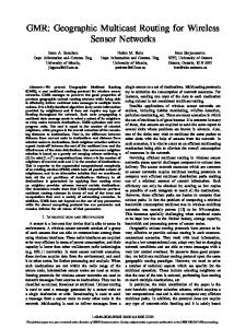
savings. As discussed in Chapter 1, sensing devices require location knowledge for data collection applications. The location information can also be leveraged by the network layer for use in routing decisions. By simply moving data geographically closer to the destination we can greatly reduce the amount of stored routing information. A problem with geographic routing is how to route around holes in the sensor field. What happens when a packet reaches a node that is not the destination, but is the closest of its neighbours to the destination? The problem with horseshoe shaped holes is depicted in Figure 2.1. In most cases, sensors that are identified purely by geographic location are easily replaceable without greatly impacting the rest of the network. Sensors Region of Interest
Sink
0 @ 68
' w" r'-.
\ @
@
Transmission Range
'
'&
@
Hole
@
@
@
@
@
@
Figure 2.1 : The problem with simple geographic routing when horseshoe shaped holes are encountered. Energy consumption is a concern in any wireless network where devices operate on battery power, however it is a particularly scarce resource in sensor networks. Sensing devices cannot be equipped with large batteries or solar panels due to size constraints. The small amount of power that is available must be stretched as thinly as possible to maximize sensor replacement cycles. Operating costs of the sensor field are reduced when sensor replacement occurs less often. As described in the previous section, reactive routing
2.2 Routing in Sensor Networks
11
schemes can be used to find optimal routes for prolonging the useful lifetime of the network as a whole. Ian Akyildiz describes the following four basic strategies for finding energy efficient paths [5]. Maximum Power Available: Sum the remaining battery power of nodes along the route.
The route with the most total remaining battery power is chosen. Minimum Hop Count: The route comprised of the smallest number of nodes is used. Minimum Energy: Select the route requiring the minimum energy to transmit the data
packets. Note that this strategy reduces to Minimum Hop Count in a homogeneous network of sensors with fixed transmission power. Maximum Minimum Power Available Node: Compare the nodes with the minimum re-
maining battery power from each route. Choose the path with the greatest such node. The number and mobility of sinks is another characteristic of the sensor field. A sole sink presents a single point of failure for the entire network. Using multiple, coordinated sinks provides redundancy against such a scenario. Assuming multi-hop forwarding, the sensors nearest to a sink will have the highest forwarding load since they are the link through which all communication for the sink must pass. When sinks are mobile this load is spread throughout the network. Thus far, the requirements of a sensor network can be met by general approaches to routing in ad hoc networks. It is the unique traffic flows present in sensor networks that are really the distinguishing factor and present an opportunity for more efficient strategies. As described in Chapter 1, data requests are distributed to the sensors by monitoring centres. When observation data becomes available, it must be routed back to the sink through sensors. Each task from a sink is directed toward a region of interest within the sensor field or the entire network (see Figure 2.2). In this scenario we have a one-to-many communication model with a sink collecting data from a group of sensors. Multicast protocols have been widely studied with respect to ad hoc networks, however the task request, data response exchange is particular to sensor networks and opens the door to efficiency gains through
2.2 Routing in Sensor Networks specialization
12
the protocols.
Region of Interest
Figure 2.2: Tasks from sinks are assigned to sensors within the region of interest. Data captured by sensors is then relayed back to the sink.
By understanding the traffic flows present in the sensor networks, we can design optimized routing protocols. Jean Carle and David Simplot-Ryl categorize sensor network applications generally as being event-driven or demand driven [2]. We go one step further to categorize the traffic flows. Triggered Data: The sink is informed whenever a particular phenomena is observed in
the region of interest. Tracking Data: The sink is given the current position of a phenomena as it moves through
the sensor field. Periodic Data: The sink periodically receives observation data from a tasked sensor. On-demand Data: Current sensor readings are immediately sent when the task is received
at the sensors. Triggered and tracking data flows correspond to the event-driven applications referred to by Carle and Simplot-Ryl. Periodic and on-demand data flows result from demand-driven applications. We assert that all data transmissions are in response to some previously received request from a sink. Sensors must be tasked even for event-driven applications.
2.3 Previous Work
13
The particular characteristics of the sensor network routing problem require focused work resulting in more advantageous solutions. Limited energy resources coupled with the necessity for operation over extended periods of time call for highly optimized protocols, potentially with the loss of generality. By identifying common traffic patterns in sensor networks we can design a routing solution that is general enough for use in varied data acquisition applications, but is highly optimized compared to general ad hoc networking answers.
2.3 Previous Work The following sections describe current routing protocols for sensor networks. The survey paper on sensor networks by Ian Akyildiz [5] contains a good overview of the state of the art in sensor network routing protocols. Given the requirements of a sensor network described in the previous section we follow the description of each protocol with a critical analysis.
2.3.1 Flooding Flooding is a well-known routing method that has been covered at length by a number of articles [5, 7, 111. Nodes in the network forward packets to all neighbours. Each packet contains a Time to Live field which is the maximum number of hops the packet is permitted to travel through the network. Duplicate messages and those whose Time to Live have expired are not retransmitted. Flooding is a brute force method for message transmission that makes no attempt at efficient resource utilization. Every node will transmit the message once. Flooding also leads to a problem called implosion. As depicted in Figure 2.3, implosion occurs when the same packet is received from multiple neighbours at the same time. The problem can cause congestion at the receiving node. Despite being wasteful of energy and causing congestion, flooding is a perfect solution with respect to fault tolerance. As long as the network is
2.3 Previous Work
14
not partitioned a packet is guaranteed to be delivered by flooding. For this reason many protocols rely on flooding in some part of their operation. Sensors
7-9
O
Figure 2.3: A sink floods a query across a sensor network. The implosion problem is highlighted in a number of places.
2.3.2 Gossiping Gossiping is only slightly more sophisticated than flooding for message routing and was developed long before the recent interest in sensor networks. Gossiping is discussed primarily in an article by Sandra Hedetniemi [7]. Nodes using a gossiping mechanism select a single neighbour at random as the next hop. Forwarding stops when the destination is reached. Gossiping is more advanced than flooding because it requires neighbour knowledge and a random selection function. Gossiping has a number of problems for routing in sensor networks. The protocol is not effective in providing the multicast communication that is often required in sensor networks. Similar to flooding, gossiping also has no regard for the energy resources in the network. Additionally, gossiping may take a long time to deliver a packet in a large sensor network. In the worst case the packet will be delivered to all sensors in the network, one at a time.
2.3 Previous Work
15
2.3.3 Small Minimum-Energy Communication Network The Small Minimum-Energy Communication Network (SMECN) protocol was developed by Li Li and Joseph Halpern [13]. SMECN is in fact a topology control algorithm rather than a routing protocol. Variable transmission power is assumed, meaning a node can increase or decrease its transmission range. This characteristic can be used to save power when required transmission ranges are short. The purpose of SMECN is to determine an efficient transmission power level for each node, with an actual routing protocol used on the topology discovered by SMECN. The algorithm begins with all sensors transmitting at maximum power. At this level the network is as connected as possible, but will also use the most energy. The protocol then follows a discovery period where transmission powers are reduced and high energy links removed. When this period has completed, each node in the network has a specific energy level at which to transmit. The stripped topology includes the minimum energy path between any two nodes. SMECN does not guarantee multiple paths between any two nodes. Only the minimum energy path between any two nodes is sure to remain. If a node on the minimum energy path fails, some nodes may become disconnected. Thus, the topology will have to be reformed as sensors fail, a costly task.
2.3.4 Sensor Protocols for Information via Negotiation The Sensor Protocols for Information via Negotiation (SPIN) take a different approach to network layer routing. The ideas behind SPIN were presented at the 1999 MobiCom conference [I I]. The philosophy is to remove the need for routing protocols by saturating the network with observations reported by all sensors. SPIN provides an energy efficient algorithm for this data dissemination. When a device in the network receives new information, either from its own sensors or from a neighbour, it advertises that information to each neighbour. The advertisement
2.3 Previous Work
16
contains only meta-data describing the observation. Each neighbour may in turn request the advertised data if it does not already have a copy. Finally, the actual observations are transmitted to each requesting neighbour. In this way, all data are propagated throughout the entire network. SPIN makes a number of implicit assumptions about the sensor field scenario. It is presupposed that all observation data in the sensor network are of interest. If this is not the case, critical resources will be wasted by disseminating unwanted information. Also, the amount of data to be gathered from the network must be very small. Otherwise the network bandwidth and device storage capacity will be quickly exhausted.
2.3.5 Sequential Assignment Routing Sequential Assignment Routing (SAR) is the routing protocol given as part of the suite of protocols for sensor networks put forth by Katayoun Sohrabi, et al. [14]. Protocols from the link layer through the transport layer are proposed in the work. Multiple tree structures are constructed across the network by the protocol. Each tree is rooted at a neighbour of the sink. Neighbours of the sink flood the network with a tree creation message, shown in Figure 2.4. The message is pushed away from the sink by forwarding to nodes at successively greater hop distances. Upon completion of the tree building process, most sensors will belong to multiple trees and thus have multiple paths back to the sink. Sensors near the sink will generally have their energy depleted at a higher rate. The multiple trees allow load balancing among these nodes. A path is selected based on available energy and QoS metrics. Sequential Assignment Routing is a robust approach for sensor networks due to the multi-path scheme used. When sensor failure occurs, a local recovery scheme is used to avoid rebuilding the entire tree. Like many other protocols, SAR requires neighbour knowledge. This type of information relies on bidirectional links. Bidirectional links are provided by sophisticated MAC layer protocols that use two-way exchanges to ensure frame reception. Such features are often not practical for use in sensor networks because of the
17
2.3 Previous Work
Sink Transmission Range Sink
Figure 2.4: Multiple trees based at each neighbour of the sink are formed by SAR.
increased overhead.
2.3.6 Low-Energy Adaptive Clustering Hierarchy Low-Energy Adaptive Clustering Hierarchy (LEACH) is a hierarchical routing protocol developed at MIT [12]. Like the SAR protocol discussed in Section 2.3.5, this work addresses the issue of sensors near the sink depleting their power resources more quickly than other sensors. As depicted in Figure 2.5, LEACH forms a hierarchical topology in which clusters of sensors communicate with the sink through cluster heads.
Figure 2.5: Routing hierarchy formed by LEACH.
LEACH forms a hierarchical topology that balances power usage across sensors over
2.3 Previous Work
18
time. The protocol begins with some members of the network randomly nominating themselves as cluster heads. A sensor becomes a cluster head with a certain probability related to its remaining energy level. Other nodes in the network join the cluster head that will require the minimum transmission power. Sensors send observed data to the cluster head. The cluster head then transmits data directly to the sink using a high power transmission. New cluster heads are selected periodically so that the high power job of cluster head is distributed among all members of the sensor field. The work implies the ability of any sensor to communicate directly with the sink using the maximum transmission power. Although this assumption is convenient for the load balancing problem, it is not realistic. The radios that have been proposed for use on sensing devices have a range of five to ten meters, far less than the imagined diameter of a sensor field.
2.3.7 Directed Diffusion Directed Diffusion provides a unique model for data collection in sensor networks. Presented at the MobiCom conference in Boston in 2000 [15], Directed Diffusion is a flexible and adaptive protocol that is able to take advantage of characteristics that may exist in the network. Directed Diffusion can also dynamically optimize the trade-off between energy consumption and fault tolerance. The algorithm uses a fairly typical exchange of sink requests and observation data. Sink request dissemination sets up gradients in the network that draw data toward the sink. If members of the network possess location knowledge, geographic routing methods may be used to direct the request toward the region of interest. Flooding is used when optimizations are not possible. Data requests are cached and may be merged with other compatible requests. When a new observation is either received from a neighbour or generated locally, the request cache is checked for a current gradient. If one is found, the data is transmitted back to the sink along the stored path. Observation data is also cached and is used for loop detection and intelligent data fusion operations.
2.3 Previous Work
19
A unique feature of Directed Diffusion is the ability to dynamically tune the level of fault tolerance. Individual paths can be either reinforced or allowed to expire based on energy or delay metrics. Using this mechanism the energy efficiency and fault tolerance needs of the network can be optimized. Unfortunately, this property requires costly periodic request retransmission.
2.3.8 Geographical and Energy Aware Routing Geographical and Energy Aware Routing (GEAR) is described in a UCLA technical paper [16]. GEAR uses location and power availability knowledge to efficiently route queries to the target region. This protocol only attempts to solve the request spreading part of the problem. Data aggregation is apparently left as future work. GEAR uses a tunable cost function in selection of the next hop for each packet. The cost function is based on the neighbour's distance to the target region and its remaining energy level. Although convergence may take some time, the hole problem described in Section 2.2 is handled. Nodes near a hole will eventually have an increased cost and present resistance to packets headed toward the hole. The protocol specifies a new method for disseminating a packet within a rectangular target region, called Recursive Geographic Forwarding. The region is recursively split into four sub-regions. The packet is sent to each of those regions using the GEAR protocol. The Recursive Geographic Forwarding mechanism is shown in Figure 2.6. A significant problem arises when either the network density is low or the transmission range is small compared to the target region size. Non-termination can occur under either of these conditions if there are no live sensors left in the target region. Routing will continually circle the target region under the assumption that a hole has been encountered.
2.3 Previous Work
20
Target Region
Figure 2.6: Query forwarding using GEAR.
2.3.9 GRAdient Broadcast The GRAdient Broadcast (GRAB) system is presented in another UCLA technical report [17]. The algorithm proposes an integrated system of density control and packet forwarding, however only the packet forwarding ideas will be explained here. A controllable mesh is used to achieve a multi-path forwarding solution. GRAB begins by building a costjield using an advertisement message flooded by the sink. The flood establishes paths to the sink after which each sensor knows its minimum cost path to the sink. Only the minimum cost path to the sink is stored. No neighbour or path information is required. The redundancy in the multi-path mesh can be varied by the data source. The source assigns each message a certain credit. An intermediate node will only forward the message if the consumed cost plus the stored cost at this node is less than or equal to the message credit. If the credit given at the source is equal to the stored cost of the minimum cost path, the message will only follow the minimum cost path. By giving extra credit, the message can follow multiple redundant paths. The cost field must be refreshed to account for changes in the network. Cost field refreshing requires another flooding by the sink. The operation is initiated when the sink
2.3 Previous Work
21
detects major changes in success ratio or traveled hop count.
GRAB effectively solves both the area coverage and data aggregation problems at the same time. The data collection portion of the system is able to balance energy consumption with fault tolerance. The cost field setup and maintenance is an expensive operation, requiring a network-wide broadcast. Fortunately it is triggered by changing network conditions rather than a blind periodic timer.
2.3.10 Two-Tier Data Dissemination A novel form of dynamic hierarchical routing has been proposed by Fan Ye, et al. [6]. The Two-Tier Data Dissemination (TTDD) protocol creates a virtual grid structure on which data is delivered. The protocol assumes the availability of location knowledge and multiple, mobile sinks. Sinks may be mobile when they are contained in hand-held devices operated
by a person walking through the sensor field. Sink mobility requires tracking their location to ensure an uninterrupted flow of data from the sources. TTDD operation is initiated by the data source through advertisements similar to those used by SPIN, described in Section 2.3.4. The source forms a virtual grid structure over the entire network and becomes the first crossing point of the grid (called a dissemination node). The advertisement is then sent to each adjacent dissemination node. Geographic
routing is used to forward packets between dissemination nodes. Each neighbour in turn forwards the advertisement to its adjacent crossing points and so on until the grid covers the entire sensor field. Since the grid is based at the source, different sources will use different dissemination nodes. A TTDD grid is shown in Figure 2.7. Following the advertisement phase, data can be requested and sent using the grid structure. Data requests are flooded by sinks within an area the size of a cell. When a query reaches a dissemination node for matching data, the query is sent toward the source using the reverse path of the advertisement. Finally, data is returned to the sink through the grid using the reverse path of the query. Routing information represents a soft-state and eventually expires. Therefore both data
22
2.3 Previous Work I
I
I
I
Source
Figure 2.7: Grid formed using TTDD source initiated advertisement.
advertisements and requests must be periodically retransmitted. Stored sink locations must expire because the sinks are mobile. As a sink moves, queries are retransmitted to find new dissemination nodes. TTDD provides a number of positive solutions to difficult problems. Provided no partitions exist, data announcement messages will reach the entire network without full-scale flooding. The use of distinct dissemination nodes by each source achieves load balancing and improves robustness and scalability because each node will hold state for no more than a few sources at a time. Unfortunately there are a number of significant drawbacks to the TTDD solution. First, the periodic signaling represents significant overhead in maintaining the grid structure. Second, failure of the single selected source could result in all data being lost from a small region of interest. Third, replication of routing information in sensors near to dissemination nodes is proposed as a way of dealing with node failure. The communication required for the replication only adds to the overhead. Fourth, TTDD does not provide a mechanism for requesting data from the sensor field. This limits the type of applications that can use TTDD to those involving triggered or event-driven data collection. Finally, the grid used by TTDD is static. If a single data source were to continuously transmit data to the sink,
2.4 Advancing the Current State of the Art
23
the network would eventually partition.
2.4 Advancing the Current State of the Art All of the routing solutions proposed to date for sensor networks have shortcomings of one form or another. In the chapters that follow we describe a new routing and addressing scheme for sensor networks called Geographic Grid Routing (GGR). The algorithm builds upon the grid construction concept used by Two-Tier Data Dissemination (TTDD) developed by Ye, et al. [6] and draws ideas from other work on both sensor networks and mobile ad hoc networks. Our work aims to address the shortcomings of previous work in the following ways. Construct a more robust grid that provides multiple paths from data source to data sink. Use sink-initiated rather than source-initiated grid construction allowing for greater data fusion opportunities. Maximize the useful lifetime of the sensor field by preferring energy efficient paths. Better distribute the data forwarding workload. Allow for greater flexibility in data acquisition through sensor tasking. The idea of tasking sensors is used by Directed Diffusion. Reduce state information to reduce storage requirements and transmissions, thereby improving scalability and performance. Permit operation in a network where bidirectional links may not exist. The preceding sections have given a broad background to the problems of request spreading and data aggregation in sensor networks. The basics of routing in ad hoc networks were explained with highlights on the similarities to sensor networks. We then covered the issues that make traffic management in sensor networks a distinct problem. Next we discussed previous solutions and exposed some of their shortcomings. In the end we
2.4 Advancing the Current State of the Art
24
gave a preview of how those weak points will be handled in our own solution. The folIowing chapter will give a more detailed description of the application domain for our work with our basic assumptions.
Chapter 3 Problem Statement, Proposed Solution and Methodology
The general context and scope of the project were given in the preceding chapters where sensor networks were introduced and previous work was described. The deficiencies of prior solutions as they relate to our problem space were also exposed. The end of Chapter 2 gave a brief glimpse of how we intend to improve upon the latest ideas for routing in
sensor networks. In particular the issues of data fusion, network lifetime, load balancing, application flexibility and network scalability will be addressed. Our own efforts stem from recent work in the field and are based on realistic assertions about the operating environment. In this chapter we define our study in greater detail and explain our approach to the issues that remain unsolved by previous efforts. Further specification of the problem domain will be provided through scope clarification, a set of assumptions and a concise problem statement. The premises having been set forth, we expand on how our algorithm overcomes the hurdles to sensor network routing. The final section of the chapter lays out the process by which we show improvement over the past endeavours.
3.1 Problem Definition
26
Problem Definition 3.1.1 Scope and Assumptions The work detailed in this thesis focuses on request dissemination and data collection from a large sensor network. It is clear from Chapter 2 that sensor networks can vary greatly in the characteristics of the network and the features offered. In this section we state the features and characteristics assumed by our work. Sensor nodes possess the following capabilities and limitations: Production costs are low and physical size is small. Otherwise deployment of a large sensor network in a range of environments would not be feasible. The power supply is restricted by sensor size. Energy consumption levels can be monitored and reported. Processing power and memory capacity are limited by cost constraints. Short-range radios are used owing to power limitations. Long-range communication is accomplished through multi-hop routing. Radio transmission power, and thus communication range, is static. High failure rates are expected due to environmental conditions and depletion of power resources. Physical location in the sensor field is fixed and known. Sink nodes can be described by the following functionality: Physical location in the sensor field is fixed and known. Energy resources are unlimited. The networking environment is assumed to conform to the listed assertions: The sensor field is represented as a two-dimensional area. Multiple sinks are deployed throughout the area of interest.
3.1 Problem Definition
0
27
Traffic flows only between groups of sensors and a sink. No sensor-to-sensor or sink-to-sink communication is required. Simple MAC layer protocols are used for energy efficiency and do not guarantee bidirectional links. Sensors are identified only by geographic position.
0
Sinks are identified by an address that is unique among all sinks in the network.
A few aspects of routing are extraneous to our specific problem. These concerns are left as future work. First, real-time data collection may well be required by many applications of the future and support at the routing layer will likely be required. Second, reliable end-to-end communication may be required for dissemination of network management directives or for some data collection types. Those issues should be handled at the Transport Layer. Finally, Quality of Service (QoS) in sensor networks relates to the resolution of the information gathered from the sensor network. Solving the QoS problem is mostly dependent on the coverage problem discussed in Section 1.3. Data fusion also affects the quality of the information received at a monitoring station. Data fusion is application dependent and is the responsibility of the application layer.
3.1.2 Statement of the Problem The constraints on the sensors and unique traffic characteristics of the network necessitate targeted research in the field of sensor networks. Much can be learned from previous work in energy efficient and multicast routing in ad hoc networks, however these general approaches fail to address the needs of sensor networks with respect to scalability, fault tolerance and device constraints. The communication of task instructions from sinks to sensors and the retrieval of data corresponding to those tasks from the sensors continues to be an area of open research. The communication must be efficient, particularly in the face of failure, and must maintain a high Level of coverage in the sensor network. The goals of energy efficiency and load balancing are viewed as orthogonal because one can only be
3.2 Solution Overview
28
optimally reached at the expense of the other. Thus satisfying both of these goals creates a challenging problem. The specific problem to be addressed is the provision of robust task dissemination and flexible collection of high resolution data from a large network of sensors such that the useful lifetime of the network is prolonged. This problem is generally known as the routing problem in wireless sensor networks. The stated assumptions and scope provide a clearly defined environment in which our solution is valid and most effective.
Solution Overview Geographic Grid Routing (GGR) is a hierarchical protocol for disseminating tasks in a sensor network and retrieving the corresponding data. Only a small subset of nodes maintain routing information and direct traffic. Other nodes simply forward traffic according to the rules of simple geographic forwarding. Simple geographic forwarding dictates that a received packet is retransmitted if the receiver is geographically closer to the destination than the sender. Due to the homogeneity of the devices, the multi-hop nature of the communication and the task specific design of the sensing devices, nodes in a sensor network take on different roles over time. The idea of role assignment in sensor networks is discussed in a paper by Manish Bhardwaj, et al. [IS]. The GGR routing protocol defines three roles for devices.
A sensor may take on more than one role at a time. Those nodes that make intelligent routing decisions are known as Dissemination Nodes (DNs). When receiving a packet for which it is not the specified destination, a sensor acts as an Intermediate Node (IN). INS only perform simple geographic forwarding operations. Finally, sensors that exist within the specified region of interest of a data request take on the role of Sensing Node (SN). The roles in a GGR network are depicted in Figure 3.1. The Dissemination Nodes in a GGR network form a virtual grid rooted at a sink. Each sink forms its own grid through which messages are routed. The grid is formed and re-
3.2 Solution Overview
29 I
r
I
I
Dissemination
Figure 3.1: Roles in a GGR network.
freshed during the task dissemination process. Thus the two-dimensional sensor field is divided into a grid of cells with a DN at each cross-point of the grid. The cross-points are equally spaced such that they are not within direct transmission range. DNs direct packets toward the next cross-point on their way to their destination. Simple geographic forwarding is used to forward messages between DNs. The virtual grid changes over time to spread the extra load associated with the DN role. The distance between grid cross-points changes in response to network conditions. Dissemination of data request messages has a dual purpose in a GGR network; grid creation and task assignment. Dissemination Nodes store the most energy efficient upstream links toward the sink as they forward data request messages and thus form the grid. The grid provides multiple paths between the region of interest and the sink, however the path with minimum used energy is favoured for communication of data back to the sink.
3.2.1 Qualitative Analysis and Comparison In this section we provide some qualitative commentary on the proposed solution and comparison to the TTDD routing algorithm, described in Section 2.3.10. The idea of a grid
3.2 Solution Overview
30
structure for routing was first used in TTDD. The many possible paths provided by the grid structure solve the problem of routing around holes in the sensor field. The problem with holes is explained in Section 2.2. The requirement for location knowledge in GGR operation does not limit the application of our solution. It is our view that location knowledge is required for any sensing application in order to make use of the data gathered by the network. In most applications it is not useful to know the data gathered from a sensor field unless the position from which it was collected is known. In this context our need for location knowledge is not an extra requirement being placed on the sensor network. Instead the GGR solution simply makes use of information already available at the application layer. The accuracy of various locationing systems cannot be guaranteed. Such errors in the reported location of a device could adversely affect the GGR protocol. The proposed routing scheme would be negatively affected if the reported location of a device can change over time. Since geographic location is used to address sensors, a changing location would be equivalent to changing the address of the sensor. Such a situation would be handled by the protocol in the same manner as a sensor failure and would hurt the performance to some degree. Consistent errors in the position reporting would negatively affect the geographic routing mechanism, however these errors are assumed to be relatively small such that geographic routing would continue to be effective. The GGR algorithm uses a number of techniques to achieve its goals of scalability, robustness and energy efficiency. Diversity injection contributes to the reliability and energy efficiency of the scheme. Diversity injection is described by Pearlman and Haas [19] and is used to select preferable routes by discovering multiple paths from a source to a destination. Scalability is achieved through the hierarchical design which uses only local knowledge in routing decisions. The hierarchical design means just a small group of nodes have to maintain routing information for a particular sink. By the same token the hierarchical design contributes to the energy efficiency because a subset of the devices in the network perform routing operations.
3.3 Methodology
31
The task dissemination used by GGR is a major advantage over TTDD for two reasons. First, sensor tasking allows for great flexibility in the type of tasks that can be handled by the network. TTDD does not provide a mechanism for sensor tasking, instead it assumes all sensors have already been tasked for event-driven data collection. Other types of data collection, such as periodic, will be important in many sensor network applications. The mechanism could also be used for distributing network management directives. TTDD does not support any form of sink initiated communication to sensors. Second, the grid used by GGR changes randomly over time to spread the role of DN over many sensors. The grid used by TTDD is static. The sink initiated approach taken by GGR provides much greater opportunity for data fusion than what exists in TTDD. Since each source in TTDD creates a grid, data from a region of interest may travel back to the sink using multiple independent grids. Data aggregation cannot occur between the different grids. GGR provides the opportunity for data aggregation at Dissemination Nodes that are shared by many data sources. An important feature of GGR is that absolutely no communication occurs unless it is either initiated by the submission of a new request or a data transmission from sensors. Our event-driven grid reconstruction technique discovers new paths only when triggered by changing network conditions.
3.3 Methodology The previous sections of this chapter defined the problem space a.nd requirements, a.nd gave a brief overview of our solution. The process by which the effectiveness of our algorithm will be shown is now explained. Three techniques will be used in this endeavour; formal verification, mathematical analysis and performance evaluation.
3.3 Methodology
32
3.3.1 Formal Verification and Analysis Prior to showing the results of simulations that model real-world conditions, we use a couple of techniques to demonstrate the validity of the Geographic Grid Routing protocol. First, we use a model checker to verify the correctness of the protocol. Second, a mathematical analysis is given to show that our algorithm is a theoretical improvement over previous work. Modeling involves constructing a prototype of the system under study. Correctness requirements of the proposed system are then formally verified through the use of a model checker. The model checker is able to prove the logical consistency of the system according to correctness properties defined by the user. Exhaustive state-space searching is used to verify the simplified model. The SPIN model checker was chosen for verification of Geographic Grid Routing. SPIN (Simple PROMELA Interpreter) verifies models specified in the PROMELA (PROcess MEta LAnguage) language. The PROMELA language and SPIN system are designed for modeling and verification of concurrent and distributed systems. The SPIN software is freely available from the Internet [20] and is explained in detail in Gerard Holzmann's book [21]. A verification by the model checker is used to verify safety properties of our system and check for invalid end-states. Our mathematical analysis explores the theoretical communication overhead and state complexity. Communication overhead indicates energy efficiency because it measures the number of transmissions required for a given operation in the sensor network. Scalability is shown through our state complexity calculations. A lower state complexity indicates that a protocol makes more efficient use of network resources and will be better able to function in larger networks or with larger regions of interest.
3.3 Methodology
33
3.3.2 Performance Evaluation Having verified the logical consistency of our design with the SPIN model checking system, the performance of the protocol must be shown. Unfortunately the deployment of a full sensor network is, at this point, beyond our means. However, there are a number of quality simulation packages available. The GloMoSim (Global Mobile information systems Simulator) [22] tool provides a full featured and realistic simulation environment for wireless communication systems. The GloMoSim simulation package was chosen for its ability to model large scale networks and its realistic radio model. The transmissions in GloMoSim may suffer from interference even when nodes are within transmission range. Under these circumstances we can measure the performance of our system in a real-world environment where unidirectional links may exist. The ability to simulate large networks is critical for simulation of sensor networks where scalability is a primary concern.
A full implementation of Geographic Grid Routing is given within the GloMoSim framework for measurement of various system properties. Metrics such as data delivery efficiency, task targeting efficiency, energy consumption and delay are studied as network size, sensor failure rate and the data collection scenario are varied. The computing resources required of our simulation are high and necessitate the use of a supercomputer. GloMoSim requires significant processing power and memory. In order to collect our detailed performance data in a timely manner, we used the Mercury Linux cluster at the University of Victoria's Research Computing Facility [23]. This is an eightyfour node cluster where each node has either 1.5 GB or 2.5 GB of memory and either dual 2.4 GHz or 2.8 GHz Intel Xeon processors. This chapter has provided a stepping stone to the rest of the thesis. A concise definition of the problem to be addressed was provided. A brief overview of our solution was given in the subsequent section. The last section was a description of the process by which enhancements over the current state of the art will be shown. The following chapters explain the GGR protocol, our analysis and performance evaluation in greater detail.
Chapter 4 Protocol Design
The preceding sections have provided motivation and background for the routing protocol described in this chapter. The problem has been clearly identified and an overview of the proposed solution has been given. The following sections specify the Geographic Grid Routing protocol for wireless sensor networks. The GGR routing protocol is a hierarchical protocol for disseminating tasks in a sensor network and communicating the corresponding data to sinks. The protocol architecture of the GGR system is depicted in Figure 4.1. The majority of our algorithm functions at the routing sublayer of the network layer. Three messages are defined at this sublayer in support of the required functionality. TASK type messages are used for grid construction and data requests. The actual gathering of observation data uses DATA and ACK type messages.
I
Application Layer Network Layer
I Routing Sublayer
MAC Layer Physical Layer ---
Figure 4.1 : GGR network architecture.
The message types used by GGR are specified in detail as they are introduced throughout the chapter. The fields of each message are given a data type. The data type can be one
35
4. Protocol Design
of those listed in Table 4.1 or a compound type. In addition, some fields may be marked with type APP meaning the data type is application dependent. Finally, some fields are actually lists of the named type. These fields are marked with the LIST modifier. Some field types may need to be adjusted to satisfy application requirements. Table 4.1 : Basic type definitions.
7 Definition
BOOL
Single bit, either 1 or 0.
INT8
Signed 8-bit value.
UINT8
Unsigned 8-bit value.
INT 16
Signed 16-bit value.
UINT 16
Unsigned 16-bit value.
INT32
Signed 32-bit value.
UINT32
Unsigned 32-bit value.
FLOAT
32-bit floating point value.
As stated in Section 3.2, the GGR protocol defines various roles for sensors in the network. Each role in the GGR network corresponds to responsibilities at a layer from Figure 4.1. Sensing Node (SN) operations occur at the application layer. The functions of the Dissemination Node (DN) happen at the routing sublayer of the network layer. Intermediate Node (IN) activities are performed at the link sublayer of the network layer. The DN, SN and IN roles that are assigned to sensors represent their state in the network with respect to a particular sink. Roles assigned by other sinks are independent. Whether or not a sensor has been assigned the SN role embodies its application layer status. The SN role is taken on when the sensor is located inside the named target region of a TASK message. Application layer state is independent of the network layer state. At the network layer, a node is either in the DN or IN state, as depicted in Figure 4.2. Sensors begin in the IN state for all sinks by default and must be promoted to the DN state. This in no way implies that state information must be stored for each sink in the network by each
4.1 Sequence Number Usage
36
sensor. The advantage of using geographic routing is that the IN role requires no state information. DN assignment occurs via reception of a TASK message where the sensor is the closest known node to the intended grid cross-point. Note that a sink always has the role of Dissemination Node and never has the role of Sensing Node. Receive TASK message [Node is closest to DP]
Receive TASK message [Node is no longer closest to DP] Figure 4.2: High level state transitions of the network layer.
4.1 Sequence Number Usage There are two distinct and unrelated sequence numbers used at the two sublayers of the GGR system. A SNP sequence number is maintained at the link sublayer and is incremented after each transmission by a Dissemination Node. The SNP sequence number is not incremented when simple geographic forwarding is performed by an Intermediate Node. A GGR sequence number is maintained by each sink and is used at the routing sublayer. The GGR sequence number is incremented after the sink sends a new TASK message to all necessary recipients. Maintaining and comparing sequence numbers requires some type casting. Sequence numbers are to be treated as unsigned values when they are incremented so that rollover occurs correctly. However, comparing sequence numbers must be done using signed arithmetic. A received message is considered new if its sequence number minus the currently
4.2 Link Sublayer Operation
37
stored sequence number results in a positive number. Otherwise the message must be discarded.
4.2 Link Sublayer Operation All the messages are prefixed with a Sensor Network Protocol (SNP) header at the link sublayer. The format of the SNP header is provided in Table 4.3. The compound type POSITION is defined in Table 4.2. The format of the POSITION fields assume a locationing technology such as GPS where X and Y coordinates are given in terms of a floating point latitude and longitude. Other schemes may be used and the format of the POSITION fields changed accordingly. Table 4.2: Compound type POSITION definition.
Description
Field Type
Field
X
FLOAT X coordinate on the two-dimensional plane.
Y
FLOAT Y coordinate on the two-dimensional plane.
Type
Table 4.3: SNP Header Definition. Description
Destination POSITION
Next DN.
Sender
POSITION
Sender of this message (last DN).
LastHop
POSITION
Last IN to handle the packet.
SeqNum
INTI6
Sender's sequence number.
Type
UINT8
Message type. Must be one of TASK, DATA or ACK.
Activities at the link sublayer are common to all nodes regardless of the type of message being sent or the role of the sensor. Referring to Table 4.3, the Destination and Sender fields
4.3 Grid Construction
38
are never modified by the link sublayer. These fields are specified at the routing sublayer by Dissemination Nodes. The Sender field always gives the position of the last DN to forward the message. The Last-Hop field of the SNP header is always set to the local position at the .C-
link sublayer prior to forwarding the packet. The SeqNum field is only set to the next SNP sequence number when the message originates from higher layers (i.e. a message being sent by a DN). A message that is simply being forwarded closer to the Destination is not modified other than the LastHop field. The Type and Payload fields are for use by the routing sublayer.
Grid Construction GGR uses a forwarding grid to route messages back to the sink. The parts of the grid are
shown in Figure 4.3. The grid is established during the task assignment phase. Cross-points of the grid are called Dissemination Points (DPs). The size of the cells is determined by the sink such that DPs are not within direct transmission range. The sink's position is the first DP. Knowing its own position and the size of each cell, the sink is able to send a TASK message to each adjacent Dissemination Point in the grid. Simple geographic forwarding is used to reach these locations. Upon receiving the TASK message, the closest known node to each DP promotes itself to become a Dissemination Node (DN). Next, the DN forwards the TASK message to each of its adjacent DPs, except the point from which the TASK message was received. These action are repeated as the TASK message propagates and Dissemination Nodes are chosen throughout the sensor field. At the same time, the
DN records the sender as an upstream link in its routing table, creating the forwarding grid. The grid provides multiple paths between the region of interest and the sink. However, as will be described later, special procedures are used to maintain loop freedom and to favour the least costly path for communication of data back to the sink.
4.4 Sink Operation
-
39
Cell Size I
2
k.I
F'
Dissemination Sink
Dissemination Nodes Region of Interest Sensing Nodes
-
TASK Message Dissemination
Figure 4.3: Grid construction and roles in a GGR network.
4.4 Sink Operation 4.4.1 Task Assignment Sensors in the network must be assigned a task before data can be gathered. A sink initiates task assignment by propagating a TASK message. The message is sent to the four nearest DPs to initiate construction of the grid. Simple geographic routing is used to route a message between sources and destinations that are not within direct transmission range, as shown in Figure 4.4. Sending to multiple locations with a single message using geographic routing adds unwanted complexity so the TASK message is sent four times. In each message the Destination field of the SNP packet is set to the location of the target DP. Adjacent DP locations are calculated as the cell size added to the current sink location in each direction. A new cell size is randomly selected from the range MIN-CELLSIZE to MAX-CELLSIZE whenever the grid is rebuilt. The Type field of the SNP header is set to TASK and the Payload is the contents of the TASK message. The TASK message is used to carry data requests from sinks to sensors. The fields
4.4 Sink Overation
40
Sink Dissemination Nodes
Figure 4.4: Task sending by a sink using simple geographic routing to reach DNs.
of the TASK message are defined in Table 4.6. Two compound types are also introduced in Tables 4.4 and 4.5. The REGION type simply defines a rectangular area as a geocast target. Fields of type TASKDEF describe a single task and all request information for the application layer. The type of the CellLSize field of the TASK message and the X-Offset and Y-Offset fields from the REGION type definition are given as FLOAT for consistency with the previous assumption of a GPS type locationing system. The units in such a system are degrees of latitude and longitude and require floating point values to precisely address regions of the sensor field. Table 4.4: Compound type REGION definition.
Field Type
Description
PI
POSITION
A corner point of the region.
P2
POSITION
Corner point opposite PI.
The fields of the TASK message should be set by the sink in the following way. The Sink-Id is set to the unique identifier for the sink. S e q B u m is set to the next GGR sequence number for the sink, which is incremented when a new TASK message is propagated through the network. The randomly chosen cell size is written to the Cell-Size field. The
41
4.4 Sink Operation Table 4.5: Compound type TASKDEF definition.
Description
Field
Type
Target
REGION Target region for this task.
Description APP
Application specific task description.
Flood field is set to zero. The Rebuild field is set to zero unless the message was triggered by the event-driven reconstruction subsystem described in Section 4.4.2. UsedEnergy is also set to zero since the sink is assumed to have infinite energy reserves. Hop-Cnt is set to zero by the sink because it is the first hop. Num is set to the number of tasks contained in the Tasks field. Each entry in the Tasks field contains a single task description. The definition of the region of interest for the task is stored in the Target field. The Description field is set to the task description given by the application layer.
4.4.2 Event-Driven Grid Reconstruction In order to spread the energy consumption load associated with the DN role, the sink must eventually build a new grid and assign the DN role to other sensors. GGR does this in an event-driven fashion similar to the scheme used by GRAB [17] and described in Section 2.3.9. In addition to its primary purpose of moving data from sensors to sinks, the DATA message is also used to trigger grid reconstruction by the sink. The fields of the DATA message are defined in Table 4.7. The UsedBnergy and Hop-Cnt fields of each DATA message allow the sink to compute the mean energy use at DNs traversed by the DATA packet. The sink stores a running average of the mean energy consumption at Dissemination Nodes using the last GRID-REBUILD-WINDOW DATA messages received. Grid reconstruction takes place when this running average has increased by GRIDIIEBUILD-THRESHOLD percentage points since the grid was built. A new TASK message is sent when it is determined that the grid needs to be rebuilt.
4.5 Intermediate Node Operation
/ Field
42
Table L 5: TASK Message Definition.
Type
Description
Assigning sink identifier (unique in this network). UINT I 6 I INTI 6
Sink's GGR sequence number.
Cell-Size
FLOAT
Size of cells in the grid being constructed.
Flood
BOOL
Set when inside the region of interest to indicate that flooding rather than grid construction should be used to propagate the message.
Rebuild
BOOL
Set when the purpose of this message is to rebuild the grid. The message is not actually delivered to sensor applications.
Usedhergy
Additive used energy percentage at visited DNs.
Hop-Cnt
Number of DNs visited.
Num
Number of tasks in this message.
Tasks
TASKDEF List of Num task definitions. LIST
The message contains all active tasks and has the Rebuild field set. The message is then sent as previously described, but using a new random cell size. In this way a new grid using different DNs is created. Figure 4.5 shows the impact of the changed cell size on DN selection. The need to balance the load of the DN role was discussed by Ye, et al. [6]. If no active tasks exist, no message is sent by the sink.
4.5 Intermediate Node Operation An Intermediate Node (IN) is any node that is not the SNP Destination of a packet. INS perform simple geographic forwarding between DNs. No state information is required for geographic forwarding. All nodes are capable of performing IN functions.
4.6 Dissemination Node Operation
43
Table 4.7: DATA Message Definition.
Field
Type
Description
Source
REGION
Source region from which this data originated.
Sinkld
UINT16
Destination sink (unique in this network).
Seqaum
INTI 6
Corresponding TASK GGR sequence number from sink.
I
I
UsedEnergy
UINT32
Additive used energy percentage at traversed DNs.
Hop-Cn t
UINT8
Number of DNs traversed.
Data
APP
Application specific data.
When a packet is received, the SNP Sender and SeqNum fields are checked to see if the packet is new. If the IN is within transmission range of the Destination, the message is passed to the routing sublayer for processing. The LastHop field is replaced with the INS own position and the packet is retransmitted if the node is closer to the Destination than the LastHop, but not within transmission range. Otherwise the packet is dropped.
4.6 Dissemination Node Operation Dissemination Nodes (DNs) fill a critical role in the sensor network. All routing operations are performed by DNs. Routes formed by nodes with relatively low remaining energy resources will be avoided in favour of higher energy routes. In this way low power nodes are saved for the more critical sensing tasks. Each DN stores a table of information used in routing decisions. The routing table format is shown in Table 4.8. The Seqfium field stores the most recent GGR sequence number received from the sink. Upstream is a list of upstream Dissemination Nodes that can be used to reach the sink. In each Upstream entry, the Usedznergy field is the total used power of the path to the sink and Hop-Cnt is the number of hops to the sink along the given route. Other fields have the same meaning as identically named fields of the TASK
44
4.6 Dissemination Node Operation
Dissemination Nodes Dissemination Nodes
Figure 4.5: Different Dissemination Nodes are chosen by varying the cell size when rebuilding the grid. The same network is shown in both (a) and (b). Each is overlaid with a grid using different cell sizes to show the Dissemination Nodes chosen in each case. message. It is possible that a sensor could become a DN for more than one sink. When such a scenario arises there will be multiple entries in the routing database. There is no procedure for removing entries from the routing database because this would require extra transmissions. Stale entries are detected with GGR sequence numbers and therefore are not problematic. The number of entries in the routing table is limited by the number of sinks in the network which has been assumed small.
4.6.1 Task Dissemination and Role Assignment The handling of TASK messages is by far the most complex operation in the GGR system. TASK messages cause new upstream links to be added to the routing table. Each path has a cost calculated using Equation 4.1 where C is the path cost, E is the used energy along said path, H is the number of hops in the route and w is a weighting factor between zero and one. w allows network designers to give higher priority to either the used energy or the
45
4.6 Dissemination Node Operation Table 4.8: GGR routing table format.
Field
I"'
I TYP~
Field
Hop-Cnt Upstream
UPSTREAM
I Strikes Backed-Off
UINT8
I UINT8 BOOL
t r - t i r (a) Routing Table Format (b) UPSTREAM Field Format
hop count when paths are selected. The cost of a link is the cost of the best path available to the sink from the upstream DN. A new Upstream entry is added to the routing table only if the cost offered by the upstream DN is less than the lowest cost that can be offered to it. If a better offer can be made to an upstream DN for which a link exists in the routing table, then the Upstream entry is removed. In other words, no two DNs will ever have each other as Upstream entries in their respective routing tables.
A received TASK message is processed as described by the pseudocode in Figure 4.6. Line 18 shows how message flooding continues within the area of interest when the Flood bit of the TASK message is set. Otherwise, the receiving node must first determine whether it is the closest node to the stated Dissemination Point at line 28. This action minimizes the number of nodes that take on the role of Dissemination Node. Once it is known that this node is a DN or is inside the region of interest, a routing entry must exist for the sink referenced in the TASK message. A new routing table entry is created at line 49 of Figure 4.6 if none exists or the message is new. Old messages are considered stale and are ignored. The cost of the advertised link is examined at line 58
4.6 Dissemination Node Operation
46
/ * Global Variables */ RoutingTable rt; Position myPos; boo1 closerNodeFound; /* * Process : hand1eTaskMsg * Description: Handles reception of a TASK message. The routing table * is updated and the message is propagated as required. */ proctype handleTaskMsg(SNPHeader snpHeader, TASKMsg taskMsg) I
/ * Local variables. */ TASKMsg newTaskMsg; i n t oldMinCost; if : : (taskMsg.f lood) ->
if
This node is inside the region defined by * / ) -> / * Continue flooding taskMsg inside region of interest. */ : : e l s e -> / * Route taskMsg geographically closer to snpHeader.destination. */ goto handleTaskMsg-end fi : : e l s e -> / * We have to figure out whether we're the closest node to the * Dissemination Point. */ if : : (distance(myPos, snpHeader.destination) < distance(snpHeader.lastHop, snpHeader.destination)) -> / * Route taskMsg geographically closer to snpHeader.destination. */ closerNodeFound = false; sleep(DN-DELAY); if :: (closerNodeFound) -> goto handleTaskMsg-end : : e l s e -> skip fi : : e l s e -> closerNodeFound = true fi f i; :: (/*
* taskMsg.tasks[O].target.
/ * Check if this is a new, current or old message. */ if
(!rtEntryExists(taskMsg.sinkId)) 1 1 (taskMsg.seqNum > rt[taskMsg.sinkId].seqNum) ) -> / * New message. */ / * Create a new routing table entry for taskMsy.sinkId. At this point the * entry has no upstream links. Any old routing table entry for the sink is * replaced. */ : : (taskMsg.seqNum < rt[taskMsg.sinkId].seqNum) -> / * Old message. */ goto handleTaskMsg-end : : e l s e -> skip / * Current message. */ fi; :: (
/ * Find out current minimum cost upstream link for this sink. */ oldMinCost = COST(getMinCostLink(taskMsg.sink1d)); / * Update the cost of the message sender in the routing table. */ / * Create a new upstream link for taskMsg.sink1d in the routing table using * snpHeader.sender. */ / * Add my own cost to the taskMsg before further propagating it. */ newTaskMsg = taskMsg; newTaskMsq.usedEnerqy = qetMinCostLink(taskMsq.sinkId).usedEnerqy +
Figure 4.6: PROMELA specification of actions taken during TASK message reception.
47
4.6 Dissemination Node Overation
/* I f
*
I am a DN o r t h i s i s n o t a f l o o d TASK m e s s a g e t h e n r e m o v e a n y u p s t r e a m l i n k s t h a t h a v e a g r e a t e r o r e q u a l c o s t t o w h a t I am n o w o f f e r i n g . */
if
I I ( r t [ t a s k M s g . s i n k I d 1 . D N ) -> i n t i = 0; do : : ( i < rt[taskMsg.sinkId].upstream.length) -> if : : ( COST(rt[taskMsg.sinkId].upstream[i]) >= C O S T ( n e w T a s k M s g ) ) -> / * Remove r t [ t a s k M s g . s i n k l d ] .u p s t r e a m [ i ] . */ :: else -> i + + f i : : else -> break od : : else -> s k i p fi; : : ( !t a s k M s g . fl o o d )
/ * I f I was p r e v i o u s l y a DN, t h e n o n l y p r o p a g a t e t h e TASK m e s s a q e i f * now m a k e a b e t t e r o f f e r . O t h e r w i s e , o n l y p r o p a g a t e t h e m e s s a g e i f * t h e f i r s t n o n - f l o o d TASK m e s s a g e I ' v e r e c e i v e d . */ if ::
I can this i s
( r t [ t a s k M s g . s i n k I d ] .D N )
if :: (
COST(getMinCostLink(taskMsg.sink1d)) < o l d M i n C o s t
)
->
/ * S e n d t a s k M s g t o e a c h a d j a c e n t DP o n t h e g r i d e x c e p t t h e s e n d e r o f t h i s * TASK m e s s a g e . N e x t , f o r e a c h t a s k d e f i n i t i o n i n t a s k M s q . t a s k s w h e r e
*
p a r t o f t a s k M s g . t a s k s f i ] .t a r g e t i s i n s i d e a n a d j a c e n t g r i d c e l l , f l o o d
*
r e g i o n o f i n t e r e s t c o n t a i n e d i n t h e a d j a c e n t g r i d c e l l . Use g e o g r a p h i c
* a TASK m e s s a g e c o n t a i n i n g o n l y t h a t t a s k d e f i n i t i o n t o t h e p a r t o f t h e * f o r w a r d i n g t o r e a c h t h e s u b - r e g i o n i f n e c e s s a r y . */
: : else -> s k i p fi : : ( ! t a s k M s g . f l o o d ) -> / * S e n d t a s k M s g t o e a c h a d j a c e n t DP o n t h e g r i d e x c e p t t h e s e n d e r o f t h i s * TASK m e s s a g e . N e x t , f o r e a c h t a s k d e f i n i t i o n i n t a s k M s g . t a s k s w h e r e * p a r t o f taskMsg. t a s k s l ij . t a r g e t i s i n s i d e an adjacent g r i d c e l l , f l o o d * a TASK m e s s a q e c o n t a i n i n g o n l y t h a t t a s k d e f i n i t i o n t o t h e p a r t o f t h e * r e g i o n o f i n t e r e s t c o n t a i n e d i n t h e a d j a c e n t g r i d c e l l . Use g e o g r a p h i c * f o r w a r d i n g t o r e a c h t h e s u b - r e g i o n i f n e c e s s a r y . */ : : else -> s k i p f i;
/ * U p d a t e n o d e s t a t e . */ rt[taskMsg.sinkId].DN I= (!taskMsg.flood); handleTaskMsg-end: skip
Figure 4.6: Continued
4.6 Dissemination Node O~eration
48
to determine whether a link to the sender should be created or updated. Only a link that would provide a lower cost path to the sink is added. In this way DNs have multiple low energy paths available to the sink. The node's own cost metrics are added to the information carried by the TASK message at line 65. TASK messages essentially advertise paths toward the sink. The cost of such a path is derived from the used energy of DNs on the path and the number of hops. In order to maintain loop freedom, DNs must remove links associated with paths that have a higher cost than what the DN itself is able to offer. Pruning these high energy paths is shown at line 71 of Figure 4.6. The final action required in processing a TASK message is to forward the message on to adjacent Dissemination Points. The decision on whether or not to forward the TASK message begins at line 88 of Figure 4.6. The TASK message is propagated only if it offers a better cost than what this node had previously offered or if the message is new. The actual TASK propagation is a lot like the activity of a sink when sending a TASK message. Those procedures are detailed in Section 4.4.1. The TASK message is first forwarded to each adjacent DP except that from which it was received. The locations of adjacent Dissemination Points are calculated by adding and subtracting the CellLSize field from the received SNP Destination. The new TASK message is not sent if the calculated Destination field is less than the transmission distance away from the Sender of the received TASK message.
4.6.2 Data Forwarding Having established the reverse paths to the sink through Dissemination Nodes, data forwarding can occur. Data forwarding involves reception and forwarding of DATA messages, acknowledgment of those messages and reception of acknowledgments for messages sent. DATA message forwarding and acknowledgment is described by the pseudocode in Figure 4.7. Upon receiving a DATA packet, the local routing table is checked for upstream links to the corresponding sink. This action is shown at line 19 of Figure 4.7. If no such link
4.6 Dissemination Node Operation
49
/ * Global Variables */ RoutingTable rt; Buffer dataBuffer; Timer ackTimer; /*
* Process : handleDataMsg * Description: Handles reception of a DATA message. The DATA message is * forwarded on the cheapest upstream link. An ACK message is sent to the
* last hop. */
proctype handleDataMsg(SNPHeader snpHeader, DATAMsg dataMsg)
I
/ * Local variables. */ ACKMsg ackMsg; / * Make sure I have an active upstream link for this sink. */ if : : ((!rtEntryExists(dataMsg.sinkId)) & &
(rt[dataMsg.sinkId].upstream.length ! = 0 ) & & ( / * Not all upstream links for dataMsg.sinkId are dead. * / ) ) -> / * See if there is any space in the dataBuffer. */ if : : (!isFull(dataBuffer)) -> / * Fill in the energy metrics for the ACK message. */ ackMsg-usedEnergy = getMinCostLink(dataMsg.sinkId).usedEnergy; ackMsg.hopCnt = getMinCostLink(dataMsg.sinkId).hopCnt;
/ * Buffer DATA message. */ bufferAdd(dataMs9, dataBuffer); if : : (dataBuffer-length< BACKOFF-THRESHOLD) -> ackMsg.ackType : : else -> ackMsg-ackType = BACKOFF fi;
=
NORMAL
/ * Send ACK message. */ send(ackMsg, snpHeader.sender);
/ * Send DATA message. */ / * Update energy metrics of data message. */
dataMsg-usedEnergy += getUsedEnergy0; dataMsg.hopCnt++; do : : ( / * All upstream links for dataMsg.sinkId are backedoff. */) sleep(BACK0FF-TIME); break; :: else -> skip od; send(dataMsg, getMinCostLink(dataMsg.sinkId).position); startTimer(ackTimer, ACK-TIME) : : else -> / * Send ACK message. */ ackMsg.ackType = FULL; send(ackMsg, snpHeader-sender) fi : : else -> / * No active upstream links. */ / * Send ACK message. */ ackMsg-usedEnergy = 0; ackMsg.hopCnt = 0; ackMsg.ackType = REMOVE; send(ackMsg, snpHeader.sender) fi
->
1
Figure 4.7: PROMELA specification of actions taken following DATA message reception.
4.6 Dissemination Node Oneration
50
exists, the sender is directed not to send any further DATA messages to this node at line 57. Otherwise, the node checks if it has enough space to buffer the DATA message. Data
messages need to be buffered until they are acknowledged in case retransmission is necessary. An acknowledgment informing the sender that the DATA message could not be buffered and requesting that further DATA messages not be sent for BACKOFF-TIME ms is sent at line 52 if no buffer space is available. At line 25 the DATA message is accepted for forwarding. An ACK message is created with updated cost metrics for this DN. The contents of the ACK message is given in Table 4.9. Piggybacking cost information on ACK messages refreshes routing table information so that more accurate decisions are made in choosing minimum energy paths. The type of ACK message to be sent is chosen at line 3 1. If there are BACKOFF-THRESHOLD or more messages buffered, the sender is asked to refrain from sending further messages for BACKOFF-TIME ms. The BACKOFF acknowledgment type provides a simple flow control mechanism.
I Field
r Sinkld
Table 4.9: ACK Message Definition.
Type
Description
UINT8
Type of acknowledgment. Must be one of NORMAL, BACKOFF, FULL or REMOVE.
UINT16
Sink for which the acknowledged DATA message was
I destined (unique in this network).
I ( SNP Sequence number of the received DATA message. /
I Ack-SeqNum I INT16 I UsedBnergy I UINT32 I Additive used energy percentage at upstream DNs. Hop-Cnt
UINT8
Number of DNs visited.
I
I
Once the DATA message has been acknowledged it can be forwarded closer to the sink. The node's own cost metrics are added to the DATA message at line 40 of Figure 4.7. At line 44 the node checks if all upstream links for this sink are currently being backed off. Sending of the DATA message is delayed for BACKOFF-TIME ms in that case. Otherwise the message is sent on the lowest cost active upstream link and the acknowledgment timer
4.7 Task Dissemination Within the Region of Interest
51
is started for ACK-TIME ms. An active link is one that is not being backed off. DNs may also perform data fusion operations as discussed in Section 2.2. Aggregation of data is entirely the concern of the application layer. A plug-in architecture is suggested to allow the routing software to call application layer data aggregation functions. At the sender, either an ACK will be received or the aforementioned ACK-TIME ms timer will expire. The procedure followed by the receiver of an ACK type message is given in Figure 4.8. At line 24 the upstream link is marked as dead if the acknowledgment type is REMOVE. Otherwise the upstream link's cost metrics are updated from the ACK message. A back-off timer is started if the acknowledgment type is either BACKOFF or FULL. No DATA messages will be sent to the upstream DN until this timer expires. Finally, starting at line 42, the acknowledgment timer is stopped and the acknowledged DATA message is either removed from the buffer or retransmitted depending on the acknowledgment type. If the DATA message is retransmitted it may be sent to a different upstream DN. A series of operations are performed when the acknowledgment timer expires before an ACK message is received. These operations are shown in Figure 4.9. Starting at line 21, the strike count of the intended destination of the corresponding DATA message is incremented in the routing table. When this count reaches MAX-STRIKES the link is marked as dead and will not be used again for forwarding DATA messages. Routing loops are possible if the link is removed rather than being marked as dead. Finally the corresponding DATA message is retransmitted at line 34.
Task Dissemination Within the Region of Interest Upon reaching a region of interest, the TASK message must be disseminated to all sensors in the defined area. A different type of routing is employed when the TASK message reaches a DN whose surrounding cells contain part of the Target. Flooding is the simplest and most effective way to distribute the TASK message to all nodes within the target region. Flooding was described in Section 2.3.1.
4.7 Task Dissemination Within the Region of Interest
5
52
/ * G l o b a l V a r i a b l e s */ RoutingTable rt; Buffer dataBuffer; Timer ackTimer; Timer backoffrimer; /*
* P r o c e s s : handleAckMsg * D e s c r i p t i o n : H a n d l e s r e c e p t i o n o f a n ACK m e s s a g e . */
10
proctype handleAckMsg(SNPHeader snpHeader, ACKMsg ackMsg) {
15
/ * L o c a l V a r i a b l e s */ UpstreamEntry upstream; RoutingTableEntry entry;
/ * G e t t h e u p s t r e a m r o u t i n g t a b l e e n t r y f o r t h e s e n d e r . */ entry = g e t ~ o u t i n g ~ n t r ~ ( rackMsg.sink1d); tj if : : (upstreamEntryExists(entry, snpHeader.sender)) -> upstream = getUpstreamEntry(entry, snpHeader.sender);
20
if
(ackMsg.ackType == REMOVE) -> upstream-dead = true else -> upstream-usedEnergy = ackMsg.usedEnergy; upstream-hopCnt = ackMsg-hopCnt; upstream-strikes = 0; upstream.dead = false;
:: ::
25
if
::((!upstream.backedOff) & & ((ackMsg.ackType == BACKOFF) j 1 (ackMsg.ackType == FULL))) -> upstream-backedoff = true; startTimer(backoffTimer, BACKOFF-TIME) : : else -> skip fi
fi : : e l s e -> skip fi;
40
/ * S t o p t h e a c k T i m e r f o r t h e acknowledged m e s s a g e and h a n d l e t h e * d a t a B u f f e r . */ stopTimer(ackTimer); if : : ((ackMsg.ackType == NORMAL) I I (ackMsg-ackType== BACKOFF)) -> / * Remove c o r r e s p o n d i n g DATA m e s s a g e f r o m d a t a B u f f e r . */ : : ((ackMsg-ackType== FULL) I ( (ackMsg-ackType== REMOVE)) -> / * S e n d b u f f e r e d DATA m e s s a g e a g a i n u s i n g t h e same p r o c e d u r e s a s * h a n d l e D a t a M s g (. . . ) . */ fi
45
50
}
Figure 4.8: PROMELA specification of actions taken following ACK message reception.
4.7 Task Dissemination Within the Region of Interest
5
/ * Global Variables */ RoutingTable rt; Buffer dataBuffer; Timer ackTimer; Timer backof f Timer;
10
/* * Process : handleAckTimeout * Description: Hand1es expiration of the ackTimer . */
53
proctype handleAckTimeout() I
15
/ * Local Variables */ UpstreamEntry upstream; RoutingTableEntry entry; / * Get the upstream entry for the intended destination of the DATA message. */ entry = getRoutingEntry(rt, ackMsg.sink1d); upstream = getUpstreamEntry(/* Intended destination of DATA message. *I);
20
/ * Mark a strike against the intended destination. */ if (!upstream.dead) -> upstream.strikes++; / * Mark the upstream link as dead if it strikes out. */ if :: (upstream.strikes == MAX-STRIKES) -> upstream.dead = true :: else -> skip fi :: else -> skip fi; ::
30
/ * Send corresponding buffered DATA message again using the same procedures as * handleDataMsg (.
35
. .) .
*/
}
Figure 4.9: PROMELA specification of actions taken following an acknowledgment timeout.
4.7 Task Dissemination Within the Region of Interest
54
As defined in Section 4.4.1, a region is specified as a rectangular area. The region of interest is divided into subregions by the virtual grid structure. A single DN is only concerned with those subregions that are contained in surrounding cells. Sensors within those subregions may use the DN as the first hop when sending observation data to the sink. An extra transmission is sometimes required by DNs further than those described in Section 4.4.1 and 4.6.1 for each task for which some part of the target region is contained within a surrounding cell. In this case the Flood field is set to one. The new TASK message contains only the tasks destined for the target region. One such message is sent to each adjacent cell that contains a part of the target region. In each such message the Target is set to the sub-region contained within the destination cell. Flooding starts immediately from the DN when the DN is located inside the target region. Task dissemination by a DN near to a target region is shown in Figure 4.10.
Dissemination
Subdivided Region of Interest Dissemination
Figure 4.10: The TASK message is sent directly to subregions of the target when it is less than one cell size from the DP. The sub-regions are defined by the existing grid. The message is then flooded within the subregion.
A simple trick is needed to flood data in a network where geographic routing is em-
ployed. The Destination field of the SNP header is set to the position of the sending node.
4.8 Sensing Node Operation
55
Otherwise the packet will not be accepted for processing by higher layers in those nodes that are not within transmission range of the SNP Destination.
4.8 Sensing Node Operation Any node that is included in the Target region of a received TASK message with the Flood bit set takes on the role of Sensing Node (SN). Forwarding of these flood messages proceeds as explained in Section 4.7. Received TASK messages are processed as defined in Section 4.6.1. All offered upstream links are accepted by SNs that are not DNs because these nodes cannot form routing loops. TASK messages with the Rebuild flag set are not passed to the application layer. DATA messages originate from the SN application layer as defined by the TASK Description, but are held at the network layer for a random period of time up to MAXSENDDELAY ms. The delay helps to spread the DATA message congestion from the region of interest in time. The sending of DATA messages by SNs involves the same DATA, ACK exchange described for forwarding by DNs in Section 4.6.2.
4.9 Configuration Parameters A number of configuration parameters were defined in preceding sections. Those values are summarized in Table 4.10 along with factors that should be considered in their setting.
Table 4.10. System ConJiguration Parameters. Parameter
Description
Determinants
Minimum cell size
Sensor density, transmis-
that can be selected
sion range and network
by a sink.
area. See Section 4.4.1.
4.9 Configuration Parameters
Parameter
56
-
MAX-CELL-SIZE
GRIDXEBUILD-WINDOW
Determinants
Description -
Maximum cell size
Sensor density, transmis-
that can be selected
sion range and network
by a sink.
area. See Section 4.4.1.
Number of samples
High
used by the sink
slower reaction to depletion
in deciding when to
of energy resources in the
build a new grid.
network. Low values could
values will cause
cause grid rebuilding to be triggered by a sporadic situation. See Section 4.4.2. GRIDBEBUILD-THRESHOLD
value
High values will result in
used by the sink in
higher variance of energy
determining whether
levels
to build a new grid.
Lower values will use more
Percentage
among
sensors.
energy due to the higher frequency grid reconstruction. See Section 4.4.2. Weighting parame-
Higher values give a greater
ter used in the path
importance to total path
cost function given
used energy while low val-
in Equation 4.1. 0 5
ues put a higher priority on
'tu
_< 1
the number of hops in the route. See Section 4.6.1.
57
4.9 Configuration Parameters
Parameter
Description
Determinants
DNDELAY
Delay used by DNs
Depends on message trans-
to see if another DN
mission time and sensor
nearer to the DP can
density. See Section 4.6.1.
be discovered. Time used by DNs
Depends
to wait for an ACK
transmission
on
message time,
message after send- MAX-CELLSIZE
MAX-STRIKES
and
ing a DATA mes-
sensor density. See Section
sage.
4.6.2.
An upstream link is
Setting
of
the
marked as dead after MAX-STRIKES parameter this many consecu- depends on the efficiency tive DATA messages of the MAC layer protocol. go unacknowledged.
Higher values should be used for an unreliable MAC layer. See Section 4.6.2.
BACKOFF-TIME
DNs back-off from
Depends on the size of the
sending on an up-
data buffers and the thresh-
stream link for this
old at which a BACKOFF
amount of time af-
type ACK is triggered. See
ter a BACKOFF or
Section 4.6.2.
FULL type ACK is received.
4.9 Configuration Parameters
58
Parameter
Description
Determinants
MAXSENDDELAY
DATA
This
messages
value
depends on
the
the MIN-CELL-SIZE and
application layer are
MAX-CELL-SIZE param-
held at the network
eters as those dictate the
layer for a random
size of the cells from which
period up to this
data will be gathered. See
value.
Section 4.8.
passed
from
The action
spreads DATA message congestion in the region of interest over time.
Chapter 5 Analysis
Formal analysis of the GGR protocol is given in this chapter. Correctness properties of the protocol are proven using the SPIN model checker. The second part of the chapter provides a formal analysis and comparison of GGR and the TTDD protocol.
5.1 Protocol Verification 5.1.1 Overview of SPIN Any system is deemed correct if it meets its design requirements. However, showing a distributed system to be correct is extremely difficult due to the high level of complexity. Testing cannot show the absence of bugs and an attempt at a mathematical proof of a concurrent system quickly becomes overwhelmingly difficult for any mathematician. Implementations of these intricate systems cannot be completely verified because the state space and computational power required far exceed what any machine can currently offer. Engineering projects often use models to work through complex design problems. Properties of distributed systems can also be verified mechanically by constructing abstract models. Model checking is the technique used to exhaustively verify simplified models. The models appear as small programs written in specialized programming languages. The modeling language provides facilities for abstract specification and definition of requirements properties. A model checker is a tool for exhaustively checking the requirements under
5.1 Protocol Verification
60
all possible executions of the model. The model checker can easily find design problems related to deadlock, live-lock and constraint violations that would be virtually impossible to uncover in the full implementation. It is up to the designer to abstract a simple, but sufficient model of the system such that the proof is accurate and can be completed in a reasonable amount of time on the available computing resources. SPIN (Simple PROMELA INterpreter) is a powerful model checking tool that has been widely used for verification of communication systems. PROMELA (PROcess MEta LAnguage) is the model specification language used by SPIN. SPIN was mainly developed at Bell Labs in the eighties and nineties. In 2002 the ACM (Association for Computing Machinery) recognized SPIN with the prestigious Sofiware System Award. Today the SPIN software is freely available from the Web [20] and active development continues. During this time SPIN has amassed a broad user base in both academia and industry. The SPIN system is explained in greater detail in Gerard Holzmann's book [Zl]. SPIN has two modes of operation, simulation and verification. Simulation mode is used for debugging purposes. A single execution of the model is explored in simulation mode. A graphical interface shows message sequence charts and finite automata representations to aid in model debugging. SPIN'S verification mode explores the entire state space of the modeled system, checking correctness criteria throughout. The graphical interface includes tools for development of the correctness properties. A few verification options allow tuning for available computing resources with memory, speed and proof completeness as possible trade-offs.
5.1.2 GGR Model The SPIN model checker was used to prove a number of important characteristics of the GGR protocol. Our abstracted model focuses on the grid construction and task dissemination portions of the protocol such that the state space remains manageable for the verifier. The model provides an unambiguous specification of these portions of the GGR protocol. The PROMELA model is given in Appendix A. 1.
5.1 Protocol Verification
61
Our model covers the following parts of the protocol. TASK message propagation is modeled because the robustness of the grid construction procedure is the most complex part of the algorithm. It is also important to prove the correctness of the route discovery part of our scheme. The model includes ACK message timeouts and REMOVE type acknowledgments as these are the events that can disrupt established routes. DATA messages only affect route priorities, but cannot establish or remove paths from the network. For this reason DATA messages are not included in the model. Assertions embedded in the PROMELA code were used to verify that the following properties of the GGR algorithm hold under all possible conditions: Loop freedom. Internal routing state cannot be corrupted. 0
Correct sequence number use. Various consistency properties remain stable. No transaction can result in an unexpected end-state.
Although every effort has been made to abstract the model such that it defines the smallest sufficient model of the actual system, the state space remains large. The use of a powerful computer was required in order to exhaustively verify the GGR protocol. The Minerva supercomputer at the University of Victoria Research Computing Facility [23] provided the required resources. Minerva allows up to eight gigabytes of memory for each process. The output of the exhaustive verification on Minerva is given in Figure 5.1. Lines 1 through 15 of the output show the progression of the model checker during the verification. The type of verification is shown as a full state-space search for assertion violations and invalid end states on lines 19 through 23. The output then shows information about the state machine used to represent our model and how it was handled by the verifier on lines
25 through 3 1. Most importantly, line 25 shows that the verifier has found zero errors. It can also be observed on line 26 that the finite state machine has over fifteen million states.
5.2 Overhead Analysis
62
The section of output on lines 33 to 39 provides the memory usage statistics. Line 39 shows that the verification required roughly 2.7 GB of memory. The messages on lines 41 through 49 show that some states in our model cannot be reached by any sequence of events. These are not error messages. Our verification required approximately twenty minutes on the Minerva supercomputer.
Overhead Analysis An analysis of the communication overhead and state complexity of GGR is given in this section. GGR is compared to the TTDD protocol in which GGR has its roots and which is presented in Fan Ye's paper [6]. The efficiency and scalability of the protocols are compared. In an effort to keep the analysis simple and easy to follow we focus on the worst-case overhead for each protocol. We also attempt to do an analysis similar to that done by Fan Ye in his paper [6] for comparison purposes.
5.2.1 Model and Notations Our analysis is based on a sensor network of N devices, covering an area A. The sensor field is assumed to be square in order to simplify the analysis. The nodes are uniformly distributed in this area with a constant density d. k sinks are distributed through the sensor field. One data packet is received from each sensor in a region of interest. As previously mentioned, both GGR and TTDD use a grid mechanism for efficient communication. Each grid cell has an area of ai2 and contains n
=d-
a2 sensor nodes. The total area for regions
of interest in the network is R. Our worst-case analysis assumes that all sinks are interested in data from all regions of interest in the network. TTDD suggests a scheme whereby data from sources within close proximity to one another would elect a single sensor to act as the data source for the group. Ye's paper [6] does not give specific details on this portion of the protocol, but the idea would decrease the state complexity and communication overhead by nearly a constant factor. We ignore this
5.2 Overhead Analvsis
5
to
15
20
25
30
35
63
Depth= 726 States= le+06 Transitions= Depth= 726 States= 2e+06 Transitions= 3e+06 Transitions= Depth= 726 States= Depth= 726 States= 4e+06 Transitions= Depth= 726 States= 5e+06 Transitions= Depth= 726 States= 6e+06 Transitions= Depth= 726 States= 7e+06 Transitions= 8e+06 Transitions= Depth= 726 States= Depth= 726 States= 9e+06 Transitions= Depth= 726 States= le+07 Transitions= Depth= 726 States= l.le+07 Transitions= Depth= 726 States= 1.2e+07 Transitions= Depth= 726 States= 1.3e+07 Transitions= Depth= 726 States= 1.4e+07 Transitions= Depth= 726 States= 1.5ei07 Transitions= (Spin Version 4.1.2 -- 21 February 2004) + Partial Order Reduction Full statespace search for: never claim - (not selected) assertion violations + cycle checks - (disabled by -DSAFETY) invalid end states + State-vector 172 byte, depth reached 726, errors: 0 1.50417e+07 states, stored 6.37423e+07 states, matched 7.87839e+07 transitions ( = stored+matched) 9.88261e+08 atomic steps hash conflicts: 1.48575e+07 (resolved) (max size 2"24 states) Stats on memory usage (in Megabytes): 2767.669 equivalent memory usage for states (stored*(State-vector + overhead)) 2603.587 actual memory usage for states (compression: 94.07%) State-vector as stored = 161 byte + 12 byte overhead 134.218 memory used for hash table (-w24) 0.039 memory used for DFS stack (-m800) 2735.690 total actual memory usage
40
45
unreached in proctype (0 of 30 states) unreached in proctype (10 of 106 states) unreached in proctype (37 of 388 states) unreached in proctype line 661, "pan-in", (12 of 83 states)
injector environment sensor :init: state 83, "-end-"
Figure 5.1: Output of the SPIN model checker for an exhaustive verification of the GGR routing protocol.
5.2 Overhead Analysis
64
feature of TTDD in our analysis due to the lack of detail and the fact that we are primarily interested in the scaling of the protocols rather than constant factors. The analysis follows a pattern of developing mathematical expressions of overhead and then plotting those expressions for comparison purposes. The graphs are based on a typical sensor network scenario where k nodes/km2 and a
= 0.6 km.
=
3, N
=
1000, R
=
1 km2, A = 10 km2, d
=
100
N and R are varied to show the scalability of GGR and TTDD.
The area, A, is varied automatically with the number of nodes, N, in order to maintain the density, d. An appropriate value for the density was determined through experimentation using our simulation environment to be described in Chapter 6.
5.2.2 Communication Overhead The communication overhead analysis presented in this section studies the number of transmissions required for the two primary aspects of protocol operation, task dissemination and data collection. Expressions for the overhead of each protocol are developed, followed by comparison based on our example network. Communication of task messages in GGR requires grid construction followed by flooding within the region of interest. The flooding overhead is proportional to the number of sensors in the region of interest and is calculated as N?. There are N / n cells in the grid.
n along each edge of the network. A square sensor field is assumed so there are \ l ~ / cells Every cell has a Dissemination Node at each corner, so there are J N / + ~ 1 DNs along each edge of the network and ( J N / n
+ 1)2Dissemination Nodes in total. Assuming the simple
case, each DN makes three transmissions during grid construction. Thus construction of a grid requires 3 (@$
+
transmissions. These actions are performed by all sinks in
the worst case resulting in task dissemination overhead of:
TTDD includes no facilities for mission updates, as task dissemination is referred to
5.2 Overhead Analvsis
65
by Ye, et al. [6]. The only way to disseminate a new task to nodes in the network is to flood the entire network. It is assumed that only one sink submits a new task to the network so the mission update overhead for TTDD is proportional to the number of sensors in the network, N. Figure 5.2 shows comparisons between GGR and TTDD for task dissemination overhead. In Figure 5.2(b) it can be seen that GGR is more efficient when the region of interest is small relative to the area of the sensor field, but less efficient as the size of the region of interest grows. The TTDD overhead is constant in Figure 5.2(b) because it only depends on the number of nodes in the network and not on the size of the region of interest. The GGR overhead is predominantly lower in Figure 5.2(a) because it does not have to flood the entire network.
Number of Nodes in the Network
Total Area of Regions of Interest (krn2)
Figure 5.2: Comparison of communication overhead during task dissemination in GGR and TTDD networks. The number of transmissions are calculated (a) as the network size increases, and (b) as the area of regions of interest in the network is expanded. Data transmissions use the grid for communication in both GGR and TTDD. Our analysis disregards the possibility of data aggregation in order to simplify the calculations. There are roughly
.\/N nodes on each side of the sensor field.
Communication of a mes-
sage in the network along the straight-line path requires at most c f l
transmissions, where
5.2 Overhead Analysis 0 NUM-NODES */
/ * Definition of the TASK message fields. */ #define FLOOD 0 #define SEQ-NUM 1 #define COST 2 /*
* Function: validstate
* Description: Examines the routing tables of all nodes and returns true if * the system is in a valid state. False otherwise. *
NOTE: This was made a macro rather than an inline function so that it can which inline functions apparently cannot.
* be used as an assert(), */
/ * No routing loops. */ \ (
\ (routingTables[O].links[O].cost == MAX-COST) 1 1 \ ( \ (routingTables[l].links[O].cost == MAX-COST) & & \ (
\
(routingTables[l].links[l].cost == MAX-COST) I I \ (routingTables[O].links[O].cost > routingTables [l].links [l].cost) \
) ) ) (
\
\
\ \ (routingTables[l].links[O].cost &&
==
MAX-COST)
/ I \
~. \
(routingTables[Ol .links[O].cost == MAX-COST) & & \ ( \ (routingTables[O].links[l].cost == MAX-COST) I I \ (routingTables[l].links[O].cost > routingTables [O].links[1].cost) \ ) \ ) \ ) && \ / * The internal state of each node is sane. */ \ (routingTables[0].links[O].cost ! = 0) & & \ ( \ (routingTables[0].links[O].cost == MAX-COST) I I \ (routingTables[0].links[l].cost == MAX-COST) 1 1 \ (routingTables[O].links[0].cost == (routingTables[Ol.links[ll.cost)) I I \ (routingTables[0].links[O] .cost == (routingTables[O].links[l].cost+l)) I I \ (routingTables[0].links[O].cost == (routingTables[0].links [l].cost-1)) 1 1 \ (!routingTables[Ol.dNode) \ ) && \ (routingTables[l].links [O] .cost ! = 0 ( \ (routingTables[l].links[O].cost == MAX-COST) I I \ (routingTables[l].links[l].cost == MAX-COST) I I \ (routingTables[l].links[O].cost == (routingTables[l].links [ll .cost)) I I \ (routingTables[l].links[O].cost == (routingTables[l].links[l].cost+l)) I I \ (routingTables[1].links[O].cost == (routingTables[l].links[ll .cost-1)) I ( \ ( !routingTables[ll .dNode) \
A.l PROMELA Model (ggr.pm1)
102
/ * Enumerations. */ / * Message types. */ mtype
=
{TASK, TIMEOUT-REMOVE};
/ * Data structure definitions. */ typedef RTEntry
i byte id; byte cost;
1 typedef RoutingTable
I bit seqNum; boo1 dNode; RTEntry links[NUM-NEIGHBOURS]; 1 typedef Payload
I byte data[MAX-PAYLOAD-SIZE]; 1
/ * Global data structures. */
/ * Channels for communicating with sensors. */ chan channels[NUM-CHANS] = [CHAN-BUFFER-SIZE] of {mtype, byte, byte, Payload) / * List of neighbours for each node. */ RoutingTable routingTables[NUM-NODES];
/ * Inline function definitions. */
/*
* Function: sendForged
* Description: Used to send on an unreliable channel with a faked source. */ inline sendForged(type, dest, src, payload)
I
atomic
t if ::
true -> channels [dest]!type, dest, src, payload
: : skip
fi
I
1 /*
* Function: send
* Description: Used by all sensors to emulate sending on an unreliable * channel. */ inline send (type, dest, payload) t sendForged(type, dest, id, payload) 1
A.l PROMELA Model (ggr.pml)
103
/*
* Function: r e c v * D e s c r i p t i o n : Used b y a l l sensors t o r e c e i v e message from t h e channel. *
Only used f o r API c o n s i s t e n c y w i t h t h e send f u n c t i o n .
*/ inline recv(type, src, payload) I
ch?type, eval (id), src, payload
1 /*
* Function: flood * D e s c r i p t i o n : Used b y sensors t o flood a */
T A S K message.
inline flood (payload, src, counter) {
atomic
I
assert (payload.data [SEQ-NUM]
if
-> sendForged(TASK, counter, src, payload) :: else -> skip fi; counter++ : : else -> break od; : : (counter != id)
/ * Reset l o c a l v a r i a b l e s t o reduce s t a t e space. */ counter
=
0
}
1 /*
* Function: propagate
* D e s c r i p t i o n : Used b y sensors t o send a
TASK message t o a l l o f i t ' s
* neiqhbours except t h e source which i s t h e node from which t h e message was * received. */ inline propagate(src, payload, counter) {
atomic
I
assert (payload.data [SEQ-NUM]
flood (payload, id, counter); : : skip
fi ; counter = 0; payload.data[FLOOD]
=
false;
*/
A.1 PROMELA Model (ggr.pm1)
104
/ * Send TASK messages. */ do : : (counter < NUM-NEIGHBOURS)
->
if
(routingTables[id].links[counter]. id ! = src) -> send(TASK, routingTables[id].links[counter].id, payload); : : else fi; counter++ : : else -> break od; ::
/ * Reset local variables to reduce state space. */ counter = 0
1 )
/*
* Function: rtInit
* Description: Deletes all the upstream links in the routing table. */ inline rtInit(counter)
I d-step I 1
counter
=
0;
do ::
(counter < NUM-NEIGHBOURS) ->
/ * Link is initialized with maximum cost and marked as unusable. */
routingTables[id].links[counter].cost counter++ : : else -> break od;
=
MAX-COST;
routingTables[id].seqNum = 0 ; routingTables[id].dNode = false;
/ * Reset local variables to reduce state space. */ counter
= 0
)
/*
* Function: getMinCost * Description: Finds the minimum cost of all upstream links */
inline getMinCost(minCost, counter) t d-st ep I counter = 0; minCost = MAX-COST; do (counter < NUM-NEIGHBOURS) -> assert(routingTables[id] .links[counter].cost routingTables[id].links[counter].cost : mincost); counter++ : : else -> break od; ::
A.l PROMELA Model (ggr.~ml)
/ * Reset local variables to reduce state space. counter = 0
*/
1
1 /*
* Function: clearPayload * Description: Utility function to clear all elements of a payload array.
*/
inline clearPayload(payload, counter) {
d-step i counter = 0; do : : (counter < MAX-PAYLOAD-SIZE) -> payload.data [counter] = 0; counter++ : : else -> break od ; counter = 0 ; 1 /*
* Function: handleTaskMsg * Description: Used by sensor processes to handle reception of a TASK message. */
inline handleTaskMsg(src, payload, oldMinCost, newMinCost, lastSrcCost, counter)
I
atomic {
assert (payload.data [SEQ-NUM] routingTables [id]. seqNum) -> rtInit(counter); routingTables[idl.seqNum = payload.data[SEQ-NUM] : : (payload.data[SEQ-NUM] < routingTables [id]. seqNum) -> goto handleTaskMsg-return : : else fi; ::
d-step {
/ * Find out the current minimum cost link. */ getMinCost(oldMinCost, counter); / * Update the cost metric of the sender in my routing table. */ assert (payload.data [COST] < MAX-COST) ; counter = 0; do : : (counter < NUM-NEIGHBOURS) -> if : : (routingTables[id].links[counter].id == src) -> / * Link is also marked as usable at this point. */ 1astSrcCost = routingTables[id].links[counter].cost; routingTables[id].links[counter].cost = payload.data[COST]; assert(payload.data[COST] counter++
A.l PROMELA Model (ggr.pm1)
106
fi : : else
-> break
od;
/* F i n d o u t t h e new minimum c o s t l i n k . getMinCost(newMinCost, counter);
*/
/ * O n l y r e m o v e e x i s t i n g e n t r i e s i f we a r e a l r e a d y a DN or i f t h i s i s n o t a
* f l o o d m e s s a g e . */
if :: (
(routingTables[id].dNode) I I
(
!payload.data [FLOOD]) ) ->
/ * Remove a n y l i n k s t h a t h a v e a c o s t g r e a t e r t h a n o r e q u a l t o m y n e w
* o f f e r . */ counter = 0; do : : (counter < NUM-NEIGHBOURS) -> if : : (routingTables[id].links[counter].cost >= (newMinCost+l)) -> / * S e t l i n k to MAX-COST a n d m a r k a s u n u s a b l e . */ routingTables[id].links[counter].cost = MAX-COST; : : else -> skip fi ;
counter++ -> break od : : else -> skip fi ; : : else
/ * R e s e t l o c a l v a r i a b l e s t o r e d u c e s t a t e s p a c e . */ counter = 0
/* *
less than my o l d o f f e r , t h e n update t h e c o s t i n t h e TASK m e s s a g e a n d p r o p a g a t e i t o n t h e g r i d . I f my new o f f e r i s
*/
if
(payload.data [FLOOD]) -> if : : (routingTables[id] .dNode) -> if : : (newMinCost < oldMinCost) -> flood (payload, src, counter); payload.data[COST] = newMinCost + 1; propagate (src, payload, counter) : : else -> if :: (lastSrcCost == MAX-COST) -> flood(payload, src, counter) : : else fi fi : : else -> if : : (lastSrcCost == MAX-COST) -> flood(payload, src, counter) :: e l s e fi fi : : e l s e -> if : : (routingTables[id].dNode) -> if : : (newMinCost < oldMinCost) -> payload.data [COST] = newMinCost + 1; propagate (src, payload, counter) : : else ::
A.1 PROMELA Model (ggr.pm1)
107
fi : : else ->
payload.data[COST] = newMinCost + 1; propagate (src, payload, counter) fi fi;
/ * F i n a l s t a t e u p d a t e s . */ routingTables [id] .dNode = (routingTables[id].dNode) 1 1 ( !payload.data [FLOOD]) ; /* Reset l o c a l v a r i a b l e s t o reduce s t a t e space. clearPayload(payload, counter); counter = 0; /* Return point f o r this function. handleTaskMsg-return: skip
*/
*/
1 1
/*
* Function: createTaskMsg
* D e s c r i p t i o n : C r e a t e s a random t a s k m e s s a g e .
*/
inline createTaskMsg(payload, counter) i
atomic
I if : : payload.data[FLOOD] = true : : payload.data [FLOOD] = false fi ;
if :: payload.data[SEQ-NUM] = 0 : : payload.data[SEQ-NUM] = 1 fi ;
/ * C o s t f i e l d . */ counter = 0; do : : (counter < (MAX-COST-NUM-NODES-1)) -> counter++ : : break od ; payload.data[COST] = counter;
/ * R e s e t l o c a l v a r i a b l e s t o r e d u c e s t a t e s p a c e . */ counter
=
0
I 1
/ * P r o c e s s d e f i n i t i o n s . */ /*
* Process: i n j e c t o r
* D e s c r i p t i o n : S i m p l e p r o c e s s t h a t i n j e c t s p a c k e t s i n t o the n e t w o r k a t random.
*/
proctype injector ( ) {
atomic
I Payload payload; b i t sender;
/ * C h o o s e f i r s t s e n d e r . */
i f :: sender = 0 :: sender = 1
fi;
/ * P o s s i b l y s e n d a m e s s a g e t o t h e f i r s t r e c e i v e r . */ i f : : ( n f u l l( c h a n n e l s [ O ] ) )
->
/ * S e n d a TIMEOUT-REMOVE m e s s a g e . A l l p a y l o a d f i e l d s a r e a l r e a d y c l e a r . */ sendForged(T1MEOUT-REMOVE, s e n d e r ,
( s e n d e r + l ) , payload)
:: s k i p
f i }
atomic
I
/ * P o s s i b l y s e n d a m e s s a g e t o t h e o t h e r r e c e i v e r . */ sender++; i f : : ( n f u l l ( c h a n n e l s [ l ] ) ) -> / * S e n d a TIMEOUT-REMOVE m e s s a g e . A l l p a y l o a d f i e l d s a r e a l r e a d y c l e a r . sendForged(T1MEOUT-REMOVE, s e n d e r , ( s e n d e r + l ) , p a y l o a d ) :: s k i p fi
1 }
/* * Process: environment * D e s c r i p t i o n : T h i s p r o c e s s m o d e l s a l l o t h e r s e n s o r s o r s i n k s i n the n e t w o r k * t h a t may s e n d m e s s a g e s t o t h e s e n s o r s u n d e r s t u d y a s w e l l a s o t h e r f a c t o r s * such a s timeouts o r d e l e t e messages.
*/
proctype environment(byte i d ) I
$
/* Local v a r i a b l e d e c l a r a t i o n s . bit r e c e i v e r ; Payload payload; byte s c r a t c h B y t e ; c h a n c h = c h a n n e l s [ i d ];
*/
/ * C h a n n e l a s s e r t i o n s . */ # i f (CHAN-BUFFER-SIZE != 0 ) xr c h ; / * O n l y I receive o n m y c h a n n e l . #endif
*/
/ * S a n i t y c h e c k . */ assert(MAX-COST > NUM-NODES); / * R u n t h e p r o c e s s t h a t i n j e c t s p a c k e t s i n t o t h e n e t w o r k . */ run i n j e c t o r
() ;
atomic
I
/ * C h o o s e f i r s t receiver. */ i f :: ::
receiver receiver
= =
0 1
fi;
/ * P o s s i b l y s e n d a m e s s a g e t o t h e r e c e i v e r . */ i f :: t r u e
->
*/
A.1 PROMELA Model (ggr.pm1)
109
/ * C r e a t e a r a n d o m , b u t v a l i d TASK m e s s a g e . */ createTaskMsg(payload, scratchByte); send (TASK, receiver, payload) :: skip
fi;
/* Clear l o c a l v a r s t o decrease s t a t e space. clearpayload (payload, scratchByte) ; scratchByte = 0;
*/
atomic
I
/ * R e c e i v e r i s n o w t h e o t h e r n o d e . */ receiver++; if ::
true ->
/ * C r e a t e a r a n d o m , b u t v a l i d TASK m e s s a g e . */ createTaskMsg(payload, scratchByte); send (TASK, receiver, payload) :: skip
fi;
/* C l e a r l o c a l v a r s t o d e c r e a s e s t a t e space. clearPayload(payload, scratchByte); scratchByte = 0;
*/
/ * R e c e i v e m e s s a g e s u n t i l a l l h a v e been s e n t . */ do
: : recv(-, -, payload) : : t i m e o u t -> b r e a k
-> s k i p
od
/*
* Process: sensor
* D e s c r i p t i o n : T h i s p r o c e s s m o d e l s a s i n g l e s e n s o r i n the n e t w o r k . */ p r o c t y p e sensor(byte id)
I atomic
I
/ * L o c a l v a r i a b l e d e c l a r a t i o n s . */ Payload payload; c h a n ch = channels [id]; b y t e src, scratchBytel, scratchByte2, scratchByte3, scratchByte4;
/ * C h a n n e l a s s e r t i o n s . */ # i f (CHAN-BUFFER-SI ZE ! = 0 ) x r ch; / * O n l y I receive o n m y c h a n n e l . #endif
*/
/ * F o r e v e r r e c e i v e m e s s a g e s a n d h a n d l e t h e m . */ do
recv(TASK, src, payload) -> handleTaskMsg(src, payload, scratchByte1, scratchByte2, scratchByte3, scratchByte4) : : recv (TIMEOUT-REMOVE, src, payload) -> / * I n a c t u a l i m p l e m e n t a t i o n we n o w m a r k l i n k a s u n u s a b l e . */ ::
skip : : t i m e o u t -> b r e a k
A.1 PROMELA Model (ggr.pm1)
110
/*
* Process: i n i t
* D e s c r i p t i o n : The f i r s t p r o c e s s t o s t a r t and i n i t i a l i z e t h e s i m u l a t i o n .
*
A l l o t h e r p r o c e s s e s a r e c r e a t e d from t h i s one.
*/
init 1
atomic {
b y t e i, j ,
k, id;
d-st ep
t
/ * S e t u p t h e t o p o l o g y . */ routingTables [ 01 . links [O].id routingTables[O] .links[l].id routingTables[l].links[0].id routingTables[l].links[l].id
=
= = =
1; NUM-NODES; 0; NUM-NODES;
/ * F i r s t c l e a r t h e r o u t i n g t a b l e s . */ id do
=
0;
: : (id < NUM-NODES) rtInit (i);
->
id++ :: else
-> break
od;
/ * R e s e t l o c a l v a r i a b l e s t o r e d u c e s t a t e s p a c e . */ i = 0; id = 0;
1
/ * C r e a t e a random, b u t v a l i d i n i t i a l s t a t e f o r / * S e t u p l a s t s e q u e n c e n u m b e r e n t r i e s . */ i = 0; do : : (i < NUM-NODES) -> if : : routingTables[i].seqNum = 0 : : routing~ables[i].seqNum = 1 fi; if :: ::
routingTables [i].dNode routingTables[i].dNode
= =
true false
f i;
i++ :: else
-> break
od;
/ * S e t u p c o s t e n t r i e s . */ i
=
0;
/ * L o o p t h r o u g h e a c h n o d e i n t h e n e t w o r k . */ do ::
(i < NUM-NODES) -> = 0; / * L o o p t h r o u g h e a c h n e i g h b o u r o f t h e n o d e . */ do : : ( j < NUM-NEIGHBOURS ) -> j
the n e t w o r k .
*/
A.l PROMELA Model (ggr.pm1)
111
/ * Choose t h e c o s t f o r t h i s n e i g h b o u r . */ k = 0; do : : (k < MAX-COST) -> k++ : : break od; routingTables[i].links[jJ.cost = k; / * Check i f t h i s c a u s e d a l o o p t o b e formed. */ if : : ( !validstate ( ) ) -> routingTables [i] .links[ j] .cost : : e l s e -> skip fi;
j ++ : : e l s e -> break
od; i++ : : e l s e -> break
od;
/* Insert breakpoint for simulations. print f ( "MSC: BREAK\." ) ; /* S t a r t sensor processes. run sensor (0); run sensor ( 1 ); run environment(NUM-NODES);
*/
*/
end : ( ! validstate ( ) )
-> a s s e r t (validstate( )
)
=
MAX-COST;