Geographic and Energy-Aware Routing in Wireless Sensor Networks

International Journal of Ad Hoc and Ubiquitous Computing, Vol. x, No. x, xxxx 1

Geographic and Energy-Aware Routing in Wireless Sensor Networks Dengfeng Yang† , Xueping Li§∗ , Rapinder Sawhney‡ , Xiaorui Wang [ †

Department of Industrial and Information Engineering University of Tennessee Knoxville, TN 37996-0700, USA Tel.: +1-865-974-3511; Fax: +1-865-974-3511 E-mail:([email protected]) § Department of Industrial and Information Engineering University of Tennessee 408 East Stadium Hall, Knoxville, TN 37996-0700, USA Tel.: +1-865-974-7648; Fax: +1-865-974-0588 E-mail:([email protected]) ‡ Department of Industrial and Information Engineering University of Tennessee Knoxville, TN 37996-0700, USA Tel.: +1-865-974-7653; Fax: +1-865-974-0588 E-mail:([email protected]) [ Department of Electrical and Computer Engineering University of Tennessee Knoxville, TN 37996-0700, USA Tel.: +1-865-974-0627; Fax: +1-865-974-5483 E-mail:([email protected]) ∗ Corresponding author Abstract: Energy efficiency is crucial for large scale sensor networks due to the intrinsic resource constraints of the wireless sensors and the infeasibility to change depleted batteries that may reside in hostile environments. This paper proposes an energy efficient routing algorithm based on a two-layer wireless sensor network (WSN) architecture to maximize the lifetime. The proposed scheme takes advantage of the geographic deployment knowledge to build routing protocols. Linear programming formulations are developed to maximize the lifetime of WSNs. A hybrid energy-efficient routing scheme (HERS) is proposed to incorporate both max-min residual energy and min-max communication energy consumption information. Simulation results show that the proposed routing algorithms can prolong the lifetime of a WSN compared to the existing algorithms. Keywords: Wireless Sensor Network, Geographic Deployment Knowledge, Energy-Aware Routing Reference to this paper should be made as follows: Dengfeng Yang, Xueping Li, Rapinder Sawhney, and Xiaorui Wang (xxxx) ‘Geographic

c 200x Inderscience Enterprises Ltd. Copyright °

2

Dengfeng Yang, Xueping Li, Rapinder Sawhey, and Xiaorui Wang and Energy-Aware Routing in Wireless Sensor Networks’, International Journal of Ad Hoc and Ubiquitous Computing , Vol. x, No. x, pp.xxx–xxx. Biographical Notes: Dengfeng Yang is a Ph.D. student in the Department of Industrial and Information Engineering at the University of Tennessee, Knoxville. His research interests are focused on system modeling and optimization, data storage and query for sensor network, energy efficient routing, and key management. Xueping Li is an Assistant Professor of Industrial and Information Engineering and the Director of the Intelligent Information Engineering Systems Laboratory (IIESL) at the University of Tennessee - Knoxville. His research areas include information assurance, scheduling, web mining, supply chain management, lean manufacturing, and sensor networks. He is a member of IEEE, IIE and INFORMS. Rapinder Sawhney is an Associate Professor and Associate Department Head in the Department of Industrial and Information Engineering at the University of Tennessee, Knoxville. He was the recipient of Lean Fellowship and was responsible for enhancing the competitiveness of Tennessee industry utilizing the Lean Manufacturing concept. His research interests are developing Lean methods to implement Lean, which have resulted in various publications. His experience includes working for over hundreds of organizations in implementing the Lean concept. Xiaorui Wang is an Assistant Professor in the Department of Electrical and Computer Engineering at the University of Tennessee, Knoxville. His research interests are wireless sensor networks, real-time embedded systems, distributed systems, power-aware computing, and Quality of Service (QoS) control. He is a member of the IEEE, the IEEE Computer Society and the ACM.

Geographic and Energy-Aware Routing in Wireless Sensor Networks 1

3

Introduction

Wireless sensors are autonomous sensing devices with wireless communication capability within a short distance. A sensor node typically consists of a power unit, a sensing unit, a processing unit, a storage unit, and a wireless transmitter/receiver (Akyildiz et al., 2002). A wireless sensor network (WSN) contains a large number of sensor nodes deployed in some controlled and safe environments (such as home, office, warehouse, et al.) or some uncontrolled and hostile environments (such as battlefields, toxic regions, et al.). It has wide applications that include combat field surveillance, real-time traffic and pollution monitoring, wildlife monitoring, and so on. However, several limitations must first be addressed such as energy constraints, computation capabilities and security issues for a wide practical use of sensor networks. Among these limitations, energy constraint is of great importance. The large number of sensors in the network and their random distribution in the application field and the possible hostile environment make it extremely difficult, if not impossible, to replenish the drained battery of each sensor. Therefore, how to make efficient use of the batteries and extend the lifetime of sensor networks has become one of the most important research issues of WSNs (Akkaya and Younis, 2005). Current energy-aware protocols are mainly categorized into 1) minimum energy routing protocols (Singh et al., 1998; Haque et al., 2005); 2) max-min routing protocols (Li et al., 2001; Toh, 2001; Zhang and Mouftah, 2006); and 3) minimum cost routing protocols (Chang and Tassiulas, 1999, 2000; Zhang and Mouftah, 2006; Kalpakis et al., 2002). The minimum energy routing protocols minimize total consumed energy to reach the destination thus minimizing the unit energy consumption per packet. However, these protocols may not maximize the network lifetime since the residual energy is not taken into account. Consequently, some nodes on the minimum energy routes will easily fail due to the heavy forwarding load. The max-min routing protocols, such as conditional max-min battery capacity routing (CMMBCR) (Toh, 2001), max-min zPmin (Li et al., 2001) and MREP (Zhang and Mouftah, 2006), avoid this problem by choosing a route that maximizes the minimal residual energy of some nodes in this route. But these protocols add the overhead of control packets for the on-demand version and it is difficult to decide the optimal threshold value that determines the operation modes. Besides the above three categories of energy-aware protocols, there are many other efforts to extend the lifetime of WSNs. Linear programming (LP) formulations are proposed for the network lifetime maximization (Chang and Tassiulas, 1999, 2000; Zussman and Segall, 2003; Hou et al., 2005; Kalpakis et al., 2002). Storage node placement problem is considered to save energy for data collection and data query (Sheng et al., 2006). Several upper bounds of the lifetime of a sensor network are derived (Bhardwaj and Chandrakasan, 2002; Sadagopan and Krishnamachari, 2004; Sankar and Liu, 2003). Most of the above energy-aware protocols are based on the flat network or hierarchical network and neglect the information that how the sensor nodes are deployed and distributed. The geographic location information is easy to obtain due to the very nature of a WSN and can be used to build routing algorithms to construct a scalable energy-saving communication infrastructure. An advantage of geographic routing is its stateless and localized nature since the packet forwarding

4

Dengfeng Yang, Xueping Li, Rapinder Sawhey, and Xiaorui Wang

depends only on the location information of the candidate nodes in the vicinity and the destination node. Hence, the geographic routing is scalable because it does not require additional control overhead. In this paper, we present a two-layer sensor network model by incorporating the geographic deployment knowledge of the network based on which we propose a Hybrid Energy-Efficient Routing Scheme (HERS) to extend the network lifetime by considering the max-min residual energy routing and the min-max cost routing. To the best of our knowledge, this is the first work to develop the hybrid energy-efficient routing protocol while minimizing the communication energy consumption using the nodes deployment knowledge. The rest of the paper is organized as follows. Section 2 describes the proposed two-layer network architecture and the deployment method. Section 3 provides the LP formulations of max-min residual energy and min-max cost optimization problems. A hybrid energy-efficient routing algorithm is developed. Section 4 shows the simulation results and comparisons with other similar protocols in terms of network lifetime. Finally, section 5 concludes the paper.

2 2.1

Network Architecture and Deployment Method Scheme Architecture

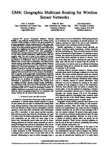
It is critical to construct and maintain an efficient network topology. The sensor nodes in a multihop WSN can collaborate with each other to determine their transmission power and define the network topology through forming proper neighbor relations. This topology differs from the ”traditional” network in which the nodes transmit with their maximal transmission power without considering the power efficiency. We define a two-layer architecture of a WSN as shown in Fig. 1, which is different from traditional flat networks such as Fig. 2. In a flat network, the topology implicitly depends on the geographic locations of the sensors and each node transmits with its maximal transmission power. Although simple for small networks, this network architecture suffers from scalability. For example, adding a new node needs to inform the whole network to set up the keys for communication, which involves large communication energy consumption and is infeasible for the WSN because of its intrinsic resource limitation. On the other hand, a WSN acts similar to scale free networks (Barab´asi and Albert, 1999), in which there is a high probability that a node links to a node that has already a large number of connections. This means that for a group of sensor nodes, there could be one or two nodes that act as communicating switches. Hence, in this paper, we introduce the concept of cluster heads and use as the switches and propose a two-layer WSN architecture Fig 1. The base station and cluster heads constitute a logical top layer while other sensor nodes constitute a logical lower layer. This two-layer group-based architecture assumption is reasonable and practical for the large-scale network. Each group contains several cluster heads to communicate with the base station. If two groups are not neighbors, the sensors will communicate via cluster heads and the base station. More details of this two-layer architecture can be found at (Li et al., 2007).

Geographic and Energy-Aware Routing in Wireless Sensor Networks

5

¿ Insert Figure 1 and Figure 2 about here. À

2.2

Deployment Knowledge

There are many methods to deploy sensor networks (Zhou et al., 2005; Du et al., 2004). For example, an airplane can scatter sensor nodes over the battlefield. Based on the above two-layer architecture and the geographic locations of the sensor nodes, we can partition a large scale sensor network into groups. The following assumptions are made: 1) Nodes are deployed randomly and the groups are allocated according to the geographic location; and 2) Once the sensor nodes are deployed, they are static. A deployment point refers to the location where a sensor node is deployed. The probability density function (pdf) of the geographic location of the nodes such as their Euclidean locations can then be estimated. In practice, sensor nodes are usually deployed in groups to realize a specified function, e.g., in (Werner-Allen et al., 2005). Sensor nodes are deployed in different groups and each group is considered as a unit to sense temperature, acoustic pressure and seismic velocity. In the paper, we adopt such a group-based deployment approach, assuming that the target deployment region is a two-dimensional ma×na rectangular area. The target region is divided into m × n equal-sized subregions Rij (i = 1, · · · m, and j = 1, · · · n) with each subregion a × a square meters. Each group, Gij (i = 1, · · · m; j = 1, · · · n), is deployed to the subregion Rij . Let N be the total number of sensors. The N sensors are uniformly partitioned into N/g groups Gij with the number of sensors in each group equal to g, and each group Gij is randomly deployed into the subregions Rij . The proposed deployment scheme relaxes the assumptions in (Du et al., 2004) so that subregions are predefined and each sensor group is deployed into a specified subregion. Every sensor node k in group Gij can be denoted as [(i, j), k ∈ N ]. The deployment knowledge can be obtained as follows: 1.

Divide the target region into subregions Rij ;

2.

N sensor nodes are partitioned into groups Gij with g sensors in each group;

3.

The node k in group Gij has an identifier [(i, j), k ∈ Gij ], and the distribution of the sensors in each group follows a pdf f (x, y|k ∈ Gij ). A natural choice for the pdf is a two-dimensional Gaussian distribution which can be easily extended to other distributions such as the Poisson distribution (Sheng et al., 2006) or the uniform distribution according to the application or the actually distribution of the sensors. In Section 4 we will investigate the influence of pdf on the maximal lifetime of the system;

4.

Randomly distribute the groups Gij into the subregions Rij .

Since we model the sensor deployment distribution as a two-dimensional Gaussian distribution, the pdf for the sensor node k in the position µ = (x, y) is deployed in the group Gij whose deployment coordination is (xi , yj ). We have the probability density function: f (x, y|k ∈ Gij ) =

1 −[(x−xi )2 +(y−yi )2 ]/2σ2 e 2πσ 2

(1)

6


where σ 2 is the variance parameter of the Gaussian distribution. ¿ Insert Figure 3 about here. À An example is shown in Fig. 3, where the target deployment region is divided into 4 × 4 sub-regions Rij (1 ≤ i ≤ 4, 1 ≤ j ≤ 4). The N sensors are partitioned into 16 subgroups Gij (1 ≤ i ≤ 4, 1 ≤ j ≤ 4), with each group containing g nodes and 3 cluster heads. These groups are randomly distributed into the sub-regions. In this deployment method, each group of sensors has eight randomly determined adjacent groups, i.e., sensors in group G32 have neighbors either in group G22 or in groups G31 , G22 , G14 , G11 , G41 , G13 , G42 , G34 , and the sub-region Rij is a square with the edge a × a. For simplicity, we assume each group has 8 neighbors and ignore the groups locating at the edge and the corner of the targeted area, where they actually have 5 and 3 neighbor groups, respectively. When the pdf f (x, y|k ∈ Gij ) of sensor nodes in the sub region Rij is as in Eq. 1, the probability that the sensor deployment point will be out of the range of the preferred targeted sub-region is less than 0.03% if we empirically choose σ to ensure 6σ = a, where σ is the standard deviation of the Gaussian distribution. For example, in the Fig. 4, σ is equal to 25m/6.

3

Maximization of the Lifetime of Network

A sensor network can be modeled as a directed graph G(N, L), where N is the set of all nodes plus the base station, and L is the set of all directed links (i, j), i, j ∈ N . Link (i, j) exists if and only if j ∈ Si , where Si is the set of all nodes that can be directly reached by node i with a certain transmit power level in its dynamic range. SU BRt (g, e) represents the directed subgraph of the tth group SU BRt , where g is the group size, or the number of sensor nodes in the group SU BRt , e is the set of all the directed links (p, q), and 0 ≤ t ≤ N/g, p, q ∈ N . The directed graph CB(M, CL) is the set of all cluster heads and the base station, where M is the set of all the cluster heads and the base station, CL is the set of all the directed links (x, y), x, y ∈ M . Let CH be the set of cluster heads. Each node i has an initial battery energy Ei . The transmission energy consumed at node i to transmit a data unit to its neighboring node j is denoted by etij and the energy consumed by the receiver j is denoted by erij . There will be multiple commodities C in this network G(N, L), where a commodity is defined as a group containing the source and destination nodes. For example, SU BRt (g, e) can be seen as a commodity, and the source nodes are the sensing nodes which will send the sensed information to the destination nodes. The destination nodes are the cluster heads, which receive the sensed information, process or relay it. Another example is CB(M, L), where source nodes are the cluster heads and the destination node is the base station. We assume that each sensor node generates one data packet per time unit, which is termed as one round, and transmits the packet to the base station via intermediate nodes. For simplicity, every packet has a fixed size of z bits. At each round, each function unit, or group, will sense the necessary information and send it to the cluster heads for data aggregation; then, the cluster heads will send


7

the extracted information to the base station. The base station is assumed to be resource rich. We define the system lifetime as the duration of time where all the function units perform properly. We assume that all the groups have to coordinate with each other to perform their designed functions. Hence, the lifetime of a WSN is equal to the time of the death of the first group after time zero. In our model, when all the 3 cluster heads use up the energy, the group will lose its function, and consequently, the system will die. The objective is to find the most energy efficient algorithm that can maximize the lifetime of the network. 3.1

Energy Model

Our general energy model follows the first order radio model (Heinzelman et al., 2000). The energy expenditure per unit of information transmission from node i to j with the distance dij is given by: etij = eT + ²amp dα ij

(2)

erij = eR

(3)

and

where eT = eR = 50nJ/bit is the energy consumed in the transceiver circuitry at the transmitter and the receiver respectively. The constant ²amp = 100pJ/bit is the energy consumed coefficient at the output transmitter antenna for transmitting one meter. The distance exponent α ranges from 2 to 4, with 2 being a short distance and 4 a long distance. We investigate the influence of α on the system’s lifetime in section 4.1. Notice that we ignore the sensing energy consumption and computation energy consumption, because they are much smaller than the communication consumption (1 : 10 ∼ 1 : 300)(Heinzelman et al., 2000). 3.2

General Energy Efficient Modeling (c)

Let qij be the transmission rate of the commodity c from node i to node j, or a flow variable indicating the flow that c sends to the base station over the link (i, j) (c) (unit bits/second), and let q¯ij be the total bits that commodity c transmits from (c)

(c)

node i to node j until time T , i.e., q¯ij = T × qij . Let CHt be the set of the cluster heads {u, v, w} in the tth group SU BRt , where 0 ≤ t ≤ N/g and u, v, w denote the 3 cluster heads in the tth group. Let ri be the necessary received flow rate for node i to finish its task (unit bits/second). Based on the lifetime definition and the system model, the lifetime of the cluster head k ∈ CHt under the given flow q (c) is given by: Tk (q) =

P j∈SRt

where

P j∈SRt

etkj

P c∈C

etkj

Ek

P c∈C

(c) qkj

+

(c) qkj

+

P j:k∈Sk

P

j:k∈Sk

erjk

P c∈C

erjk

P c∈C

(c) qjk

(c)

qjk

(4)

is the energy consumption rate includ-

ing transmitting and receiving consumptions (unit J/second). Now the lifetime of

8


our model can be defined as the minimal maximal lifetime of the cluster heads in some group, i.e.: Tsys = min max Tk (q), k∈CHt

t ∈ 1, . . . , N/g

(5)

The objective is to find the flow that maximizes the system lifetime under the flow conservation conditions. Accordingly, the energy efficiency problem can be formulated into the following linear programming problem: Maximize T

(6)

Subject to (c)

q¯ij ≥ 0, ∀j = 1, 2, . . . , N, ∀c ∈ C N +1 X

etij

j=1 N X

X

(c)

q¯ij +

c∈C (c)

N X j=1

q¯ji + ri × T =

j=1

erij

N +1 X

X

(c)

(7)

q¯ij ≤ Ei , ∀i ∈ c

(8)

q¯ij , ∀i ∈ c, i 6= j, ∀c ∈ C

(9)

c∈C (c)

j=1

where N + 1 means that we consider the base station as a packet receiver, but it is not thought of as a sensor node. Eq.(7) conserves the feature that sensors have the ability to send packets to other nodes. Eq. (8) means that any energy consumption in data sending and receiving should respect the energy constraints. Eq. (9) means that every sensor generates the same amount of bits as it takes in. As long as the variable T in (6) is considered as an independent variable, the above equations can be seen as a linear programming problem (Chang and Tassiulas, 2000). 3.3

Energy Optimization Method

In this section we first present two traditional energy optimization routing algorithms for the energy-efficient communications: one is to maximize the minimal residual energy routing path (Li et al., 2001; Toh, 2001; Zhang and Mouftah, 2006) and the other is to minimize the maximal energy consuming path (Chang and Tassiulas, 1999, 2000; Zhang and Mouftah, 2006). Then we provide our improved Hybrid Energy-efficient Routing Scheme (HERS). • Max-min Residual Energy Routing Scheme (MMRERS) To extend the lifetime of the network, MMRERS selects a routing path that contains the maximal residual energy among all the possible paths. This maximal residual energy routing path is determined in quantity by the node whose residual energy is minimal along the path. That is why the MMRERS is designed to address this max-min problem. Alternatively, the purpose of MMRERS is to find the path and maximize its remaining energy at a low communication overhead. Initially,within the group SRt , where 0 ≤ t ≤ N/g, the set A contains only the cluster heads u, v, w. Let SRt − A denote the set of sensor nodes in SRt that are not included in A. We define the residual energy of a pair (i, j) as min(Er [i] −

Geographic and Energy-Aware Routing in Wireless Sensor Networks (k)

9

(k)

etij ∗ q¯ij , Er [j] − erji ∗ q¯ji ) where i ∈ SRt − A and j ∈ A. Intuitively, on adding a directed link (i, j) to A, the residual energy at the sensor node i is reduced by the energy consumed in transmitting a data packet from i to j. Consequently, the residual energy of node j will be reduced by the energy consumed in receiving a data packet. Among all pairs (i, j) such that i ∈ SRt − A and j ∈ A, the procedure chooses one with the maximum residual energy and includes the link (i, j) in A. The process is repeated until all sensor nodes in SRt are included in A, and for other groups, the process will repeat in the same procedure. For the top layer, a similar algorithm is adopted. Firstly, the set B contains only the base station, and set CH denotes the set of cluster heads. We use the same definition of residual energy, and add the maximal residual energy link (m, n) to the set B until all the cluster heads are included in B. • Min-max Link Energy Consuming Routing Scheme (MMLERS) To maximize the lifetime of a network, a direct method is to obtain a path which consumes minimal energy in communication. Consequently, the goal of the design is to minimize the energy depleting rate at individual nodes by selecting paths constituted by links with energy as low as possible. According to our network architecture, every group contains 3 cluster heads, denoted by u, v, and w. Each cluster head needs to receive, process and transmit the information coming from every non-cluster head node within the group, which would consume the energy denoted by E. Therefore, in order to extend the lifetime T for each cluster head, our objective is to minimize the maximum energy Emax consumed by each non-cluster head node within a group. Let SRt , 0 ≤ t ≤ N/g, denote the tth group. The following is the linear programming problem to minimize the maximal energy consumption: Minimize Emax

(10)

Energy constraints: X X (c) X X (c) X etij q¯ij + erij q¯ij + j∈SRt

X

c∈C

j:i∈Si

X

erkj

k∈CHt j6=i∈Si

Flow constraints: X j∈SRt

(c)

X

(c) q¯kj

c∈C

X

etjk

∀i ∈ SRt ,

(c)

q¯jk +

c∈C

k∈CHt j6=i∈SRt

≤ Emax ,

X

0 ≤ t ≤ N/g

(11)

(c)

(12)

c∈C

q¯ji + ri ∗ T =

X j∈Si

(c)

q¯ij +

X

X

q¯ik , ∀i ∈ SRt

k∈CHt j6=i∈Si

where i is a sensor node within the group SRt , and k is a cluster head in any other groups except SRt where node i is in. For every group in the network G, the linear program minimizes the maximum energy consumed by any sensor node of this group, subjecting to the energy constraint (11) and the flow constraint (12). Eq. (12) defines the flow conservation condition, where flow in equals to flow out. For the top layer max-min problem, all the cluster heads construct another group, denoted by CH. It can be easily formulated in a similar linear equation format like Eqs. (6) - (9).

10

Dengfeng Yang, Xueping Li, Rapinder Sawhey, and Xiaorui Wang • Hybrid Energy-efficient Routing Scheme (HERS)

The MMRERS scheme suffers from the fact that the max-min residual energy links may consume more communication energy. Under this condition, the system will use up its energy soon and die. The MMLERS LP formulation can be solved polynomially by using source-based algorithms, such as Dijkstra’s algorithm or Bellman-Ford algorithm (Ahuja et al., 1993). However, its max-min paths usually contain nodes whose communication consumption to other nodes is minimal or near to minimal. Therefore, these nodes have a high probability to be selected by these optimal paths and run out of battery energy quickly due to the heavy forwarding load while other nodes contain almost full battery energy. Thus, the MMLERS is energy inefficient also. To solve these problems, we present the hybrid energy-efficient routing scheme (HERS), which considers both the max-min residual energy as the link cost and the min-max communication energy consumption. The minimum energy path will be recalculated and redirected to other paths after every residual energy broadcast, and therefore, makes good use of all the possible nodes to construct optimal paths. Also, because the algorithm runs within the divided groups, the death of a non-cluster head sensor node won’t affect the lifetime of the rest of the network. Moreover, the complexity of the HERS algorithm is low since it involves in the group size, denoted as g, and it considers the threshold values of residual energies of cluster heads. Multiple cluster heads extend the system’s lifetime also. To further investigate the impacts of residual energy broadcasting on the network lifetime, we adopt dynamic HERS, or D-HERS, which adjusts the broadcast interval, denoted by m, dynamically, and static HERS, or S-HERS, which uses a fix broadcast interval. We denote Er [i] to be the residual energy at the sensor nodes i. Initially, Er [i] = E for each node i in the network. We introduce a new link metric costij that combines the unit data transmission energy consumption etij and erji , initial energy Ei and Ej , and the residual energy Er [i] and Er [j] as follows: costij = etij (Ei /Er [i])β + erij (Ej /Er [j])β

(13)

A similar metric can be referred to in (Chang and Tassiulas, 2000). The link cost is denoted by the energy consumption from the sending nodes to the receiving nodes. We use the exponent index β to emphasize that residual energy does have impact. We will investigate the influence of the exponent index β on the system’s lifetime in section 4.1. The HERS algorithm, hence D-HERS and S-HERS which differ from each other by different residual energy broadcast policies, is describe as follows. HERS takes the deployment knowledge of N sensors and initial energy in each sensor as inputs. Output is the system’s lifetime. Let T be the system’s lifetime counted by the total rounds. During the simulation, since each group resides within a relatively small region and each contains only g nodes, we treat each group as a sensing unit which executes the same functions. Thus, we take a random selection policy to select a node to act as an information source that sends the information to the destination, or the cluster head along the optimal path. After m rounds, another random selected node is selected as the source. Similarly, another cluster head is randomly selected as the


11

Algorithm 1 HERS 1: 2: 3: 4: 5: 6: 7: 8: 9: 10: 11: 12: 13: 14: 15: 16: 17: 18: 19: 20: 21: 22: 23:

Partition the N sensor network into t ⇐ d Ng e groups gi , . . . , gt , such that each group has g nodes and 3 cluster heads. for each group, calculate the distances between each sensor node, and send the information to the cluster heads. for each cluster head, calculate the distance from other cluster heads in other groups. let initial broadcast interval m ⇐ 5 and lifetime T ⇐ 0. if mod(T, m) == 0 then for each group, broadcast the residual energy to every other node. for each cluster head, broadcast the residual energy to other cluster heads. for each group, calculate the shortest link cost paths from sensor nodes to cluster heads using Eq. 13. for each cluster head, calculate the shortest link cost paths to other cluster heads using Eq. 13. based on the new paths, for each group, send packages from sensors to cluster heads, update the residual energy. for each cluster head, send packages to other cluster heads and finally to the base station, update the residual energy. T ⇐ T + 1. else based on the old paths, for each group, send packages from sensors to cluster heads, update the residual energy. for each cluster head, send packages to other cluster heads and finally to the base station, update the residual energy. for each group if the residual energy of all the 3 cluster heads less than a threshold then return T. else T ⇐ T + 1. goto 5. end if end if

destination. For D-HERS, the broadcast interval m increments every p rounds, or time slots, where p is fixed value and is decided after the network is deployed. If m reaches the predefined threshold, it will not change any more. The time complexity of the HERS algorithm is O(tg 2 log g + t2 log t). Usually, the number of groups t is much less than the number of sensor nodes in one group g, or t ¿ g. The time complexity can be simplified as O(tg 2 log g).

4

Simulation and Results

In this section, we compare the performance of the HERS algorithm with three other algorithms: the MLDA (maximum lifetime data gathering) and CMLDA (clustering-based MLDA) which incorporate the MMRERS and MMLERS schemes

12


and are proposed by (Kalpakis et al., 2002), and the LRS Leach (Heinzelman et al., 2000; Lindsey and Raghavendra, 2002) in terms of network lifetime, since they outperform other existing energy efficiency schemes (Kalpakis et al., 2002). We build the simulation environment by choosing a 50m × 50m target area and vary the number of sensors in the network, i.e. the network size, N , excluding the cluster heads, from 40, 60, 80, to 100 respectively. Each group contains 10 noncluster head sensor nodes and 3 cluster heads. Each sensor (including non-cluster heads or cluster heads) has an initial energy of 1 unit and generates packets of size 1000 bits per round, which is consistent with the settings in (Kalpakis et al., 2002). For the lower layer, each group has an optimal path whose information source is a non-cluster-head sensor node, and destination a cluster head. For the other nodes and cluster heads within this group, they all act as information relay units and just forward the whole packets they receive to the next hop. If the next hop is a cluster head which acts as the destination, it will process these packets and extract key information and then forward them to the base station via other cluster heads. This is the top layer’s communication scheme, see next paragraph. Here we assume the extraction ratio is 1 : 10, which means in each round, a cluster head receives 1000 bits from the source node, and the key information 100 bits are extracted and forwarded to the next hop. As for the top layer, we use a similar scheme. Since N/g groups in the low layer has N/g optimal paths, and therefore has N/g information destinations, which are considered as information sources in the top layer, denoted by Pt , t ∈ 1, · · · , N/g. The destination is the base station in the top layer. According to the extraction ratio, each path will transmit 100 bits to the base station. We process these transmission in queue in our simulation, although in fact, these N/g sources may send information to the base station simultaneously. This simplification will not affect the evaluation of the algorithms since practically the base station will process incoming information in the queue, otherwise, information congest will occur. The Bellman-Ford algorithm (Ahuja et al., 1993) is used to find the optimal path, and the Boost Graph Library (Siek et al., 2000-2001) is used in our Matlab simulation code. We assume the broadcast message contains 100 bits in this simulation. The base station is located at location (25m, 150m), as (Kalpakis et al., 2002) set. We can use optimal position selection techniques to locate the base station such as in (Pan et al., 2005), but it is out of our paper’s scope. The energy model for the sensors is based on the first order radio model described in Eqs. 2 and 3. We distribute the g sensor nodes and 3 cluster heads into each group according to the Gaussian distribution, as shown in Fig. 4, where the total number of sensor is N = 40, and group size is g = 10. Therefore, there are 4 groups and each group has a 25m × 25m targeted area. We also simulate the lifetime of the network based on the uniform distribution of the sensor node in the targeted area when the network size N is 40. As shown in the Figs. 5, 6, and 7, the Gaussian distribution has a slightly better performance in the lifetime than that of the uniform distribution. ¿ Insert Figure 4 about here. À

Geographic and Energy-Aware Routing in Wireless Sensor Networks 4.1

13

Optimal Selection of Parameters

Since each node cannot know each other’s residual energy level, a periodic broadcast containing the battery energy information should be sent to the neighbors. Obviously a smaller interval will provide more accurate battery information but will also consume more communication energy and incur information congestion. A longer broadcast interval, on the other hand, will consume less energy but leads to a non-optimal path selection. Fig. 5 shows the tradeoff between the lifetime of the network and the residual energy broadcast interval. The broadcast interval ranges from 5 to 15. When m ≥ 20, the lifetime will approach to, but not exceed 16, 667, since the optimal lifetime obtained from the LP optimization is 16, 667. However, when the broadcast interval m increases, the computation time increases. We choose the broadcast interval m = 10 for S-HERS in the later discussion. ¿ Insert Figure 5 about here. À Fig. 6 shows the relation of the exponent index β in the link cost equation 13 with the lifetime of the network when the network size is 40. As we can see, the Gaussian distribution has a better performance than the Uniform distribution, and the maximal lifetime is 8529 when β is chosen to be 10. ¿ Insert Figure 6 and 7 about here. À Fig. 7 shows the impact of the exponent α in the energy equations (2)-(3) to the lifetime of the network with the network size 40. When α increases from 2 to 3, the lifetime decreases dramatically since the energy exponent change will incur changes exponentially. To compare with (Kalpakis et al., 2002), the same energy exponent α = 2 is chosen. The relationship between the network lifetime and the number of cluster heads is revealed in Fig. 8. It can be seen that the network lifetime increases with the increase of number of cluster heads. We also investigate the average number of hops per path with the cluster heads per group changing from 1 to 5. We find out that the average number of hops increases with the increase of the number of cluster heads as well which is reasonable since data packets are more likely to be relayed through the cluster heads. The increase of the number of hops may result in the degradation of the timeliness performance and higher possibility of exposition to adversarial attacks. Details of the quantitative survivability analysis of a WSN can be found at LGKE (Li et al., 2007). Hence, the selection of the number of cluster heads needs to take into account of both resource consumption and survivability. We choose three cluster heads to conduct the numerical experiment in this paper. ¿ Insert Figure 8 about here. À

14 4.2

Dengfeng Yang, Xueping Li, Rapinder Sawhey, and Xiaorui Wang Performance of HERS

In this section, we will compare the performance of HERS with CMLDA, a clustering-based 2-level hierarchical protocol proposed by Kalpakis, Dasgupta and Namjoshi (Kalpakis et al., 2002), and LRS, a chain-based 3-level hierarchical protocol proposed by Lindsey, Raghavendra and Sivalingam (Lindsey et al., 2001) since these protocols have the similar hierarchical network structure and outperforms other protocols in terms of system lifetime. More details about the protocols can be found in (Lindsey et al., 2001), (Lindsey and Raghavendra, 2002) and (Kalpakis et al., 2002). ¿ Insert Table 1 about here. À Table 1 is based on the fixed broadcast interval m = 10 for S-HERS, β = 5 and α = 2, for D-HERS, Broadcast intervals are chosen as m = 10 for N = 40, m = 12 for N = 60, m = 14 for N = 80, m = 16 for N = 100 separately. Some key observations can be obtained as follows. The lifetime of a network obtained using the static broadcast interval (S-HERS) decreases when the network size increases. It is inferior to MLDA and CMLDA when network size is 80 or more, since when the network size increases, the number of the groups increases. Therefore, the communication within the top layer consumes more energy. S-HERS performs 1.10-1.31 times better than MLDA and CMLDA with a smaller network size. The lifetime obtained using S-HERS is significantly longer than that of LRS for all the network sizes, which is 1.23-1.53 times better than LRS. D-HERS outperforms MLDA, CMLDA, and LRS at a relatively stable level of about 8500. The lifetime of the network using D-HERS is about 1.03-1.29 times longer than that of MLDA and CMLDA, and about 1.50 times longer than that of LRS. Next we conduct a series of experiments with a relatively larger network size. The sensors are deployed in a 100m × 100m targeted area based on Gaussian distribution. The network size, N , varies from 100, to 500. Each sensor has an initial energy 1 unit, and the base station is located at (50m, 300m). The network is divided into groups, and each group has 10 sensor nodes. All the settings are the same as (Kalpakis et al., 2002). In this series experiments, we adopt D-HERS scheme since D-HERS has a better performance than S-HERS in large scale networks. The results are shown in Table 2. As we can see, D-HERS has a stable lifetime level about 7200, which is about 1.1-2.0 times longer than that of CMLDA, and about 2.50 times longer than that of LRS. ¿ Insert Table 2 about here. À

5

Conclusion

Sensor networks is becoming ubiquitous, and its energy efficiency issue is crucial for its wide applications due to its intrinsic resource constraints. In this paper, we


15

tackle the energy efficiency problem by proposing a geographic and energy-aware routing protocol. Geographic deployment information of the sensors is modeled based on a two-layer sensor network. Linear programming formulations for the network lifetime maximization is developed. We propose two heuristic algorithms, S-HERS and D-HERS, to extend the network lifetime by incorporating the max-min residual energy scheme and the min-max communication energy scheme. The simulation results show that the D-HERS outperforms the existing algorithms consistently. For small scale sensor networks, the S-HERS can achieve network lifetime 1.1 − 1.3 times longer than other existing protocols. For all the networks tested with different sizes, the D-HERS can obtain about 10% − 100% increase in network lifetime comparing to its peers. Also, we find that the Gaussian deployment model prolongs the lifetime of a WSN by about 20% longer than the uniform deployment model. As part of our future research, we would like to implement the D-HERS algorithm on a real WSN using Berkeley motes. Also, this study, and those in the literature (Kalpakis et al., 2002; Lindsey et al., 2001), consider up to 500 nodes in the network. It is of interest to investigate the energy-aware routing algorithms for a large scale network, e.g. one containing more than 10, 000 nodes. References Ahuja, R. K., Magnanti, T. L., Orlin, J. B., 1993. Network flows: theory, algorithmes, and applications. Prentice Hall, Inc. Akkaya, K., Younis, M., 2005. A survey on routing protocols for wireless sensor networks. Ad Hoc Networks 3, 325–349. Akyildiz, I., Su, W., Sankarasubramaniam, Y., Cayirci, E., 2002. Wireless sensor networks: a survey. Computer Network 38, 393–422. Barab´asi, A., Albert, R., October 1999. Emergence of scaling in random networks. Science 286. Bhardwaj, M., Chandrakasan, A. P., 2002. Bounding the lifetime of sensor networks via optimal role assignments. IEEE INFOCOM. Chang, J.-H., Tassiulas, L., September 1999. Routing for maximum system lifetime in wireless ad hoc networks. the 37th Annu. Allerton Conf. Communication, Control, and Computing. Chang, J.-H., Tassiulas, L., March 2000. Energy conserving routing in wireless ad hoc networks. Proc. IEEE INFOCOM, 22–31. Du, W., Deng, J., Han, Y. S., Varshney, P. K., March 2004. A key management scheme for wireless sensor networks using deployment knowledge. IEEE INFOCOM. Haque, I. T., Assi, C., Atwood, J. W., October 2005. Randomized energy aware routing algorithms in mobile ad hoc networks. MSWim’05, Montreal, Quebec, Canada.

16


Heinzelman, W., Chandrakasan, A., Balakrishnan, H., January 2000. Energyefficient communication protocol for wireless microsensor networks. The Hawaiian Int. Conf. Systems Science. Hou, Y. T., Shi, Y., Sherali, H. D., Midkiff, S. F., September 2005. On energy provisioning and relay node placement for wireless sensor network. IEEE Trans. on Wireless Communications 4 (5). Kalpakis, K., Dasgupta, K., Namjoshi, P., 2002. Efficient algorithms for maximum lifetime data gathering and aggregation in wireless sensor network. Computer Network. Li, Q., Aslam, J., Rus, D., July 2001. Online power-aware routing in wireless ad-hoc networks. Proceedings of MOBICOM. Li, X., Yang, D., Sawhney, R., 2007. Layered group key establishment for wireless sensor networks. Pervasive and Mobile Computing, in review. Lindsey, S., C.Raghavendra, Sivalingam, K., April 2001. Data gathering in sensor networks using energy delay metric. International Workshop on Parallel and Distributed Computing Issues in Wireless Networks and Mobile Computing, (San Francisco, CA). Lindsey, S., Raghavendra, C. S., 2002. Pegasis: Power-efficient gathering in sensor information systems. Proc. of IEEE Aerospace Conference. Pan, J., Cai, L., Hou, Y. H., Shi, Y., Shen, S. X., September 2005. Optimal basestation locations in two-tiered wireless sensor networks. IEEE Trans. on Mobile Computing 4 (5), 458–473. Sadagopan, N., Krishnamachari, B., 2004. Maximizing data extraction in energylimited sensor networks. IEEE INFOCOM. Sankar, A., Liu, Z., 2003. Maximum lifetime routing in wireless sensor networks. Proc. IEEE INFOCOM. Sheng, B., Li, Q., Mao, W., May 2006. Data storage placement in sensor networks. In: ACM International Symposium on Mobile Ad Hoc Networking and Computing (Mobihoc). Florence, Italy, pp. 344–355. Siek, J., Lee, L.-Q., Lumsdaine, A., 2000-2001. Boost graph libraryHttp://www.boost.org/libs/graph/doc/index.html. Singh, S., Woo, M., Raghavendra, C., October 1998. Power-aware routing in mobile ad hoc networks. Proc. ACE/IEEE MOBICOM98. Toh, C. K., June 2001. Maximum battery life routing to support ubiquitous mobile computing in wireless ad hoc networks. IEEE Communication Magazine, 138– 147. Werner-Allen, G., Johnson, J., Ruiz, M., Lees, J., Welsh, M., January 2005. Monitoring volcanic eruptions with a wireless sensor network. In Proceedings of the Second European Workshop on Wireless Sensor Networks (EWSN’05).


17

Zhang, B., Mouftah, H. T., 2006. Energy-aware on-demand routing protocols for wireless ad hoc networks. ACM Wireless Networks 12, 481–494. Zhou, L., Ni, J., Ravishankai, C. V., September 2005. Efficient key establishment for group-based wireless sensor deployments. Proceedings of 2005 ACM Workshop on Wireless Security (WiSe 2005). Zussman, G., Segall, A., 2003. Energy efficient routing in ad hoc disaster recovery networks. Proc. IEEE INFOCOM.

18


List of Tables 1 2

Simulation results for a 50m × 50m sensor network . . . . . . . . . . Simulation results for a 100m × 100m sensor network . . . . . . . . .

19 20

Geographic and Energy-Aware Routing in Wireless Sensor Networks Table 1

19

Simulation results for a 50m × 50m sensor network

N

S-HERS

40

8529

60

7912

80 100

D-HERS

MLDA

CMLDA

LRS

6610

6512

5592

8468

7174

7084

5872

7397

8471

7945

7809

6002

6804

8545

8290

8121

5526

8529

S-HERS broadcast interval m = 10 D-HERS Broadcast interval m = 10 for N = 40, m = 12 for N = 60, m = 14 for N = 80, m = 16 for N = 100

20 Table 2

Dengfeng Yang, Xueping Li, Rapinder Sawhey, and Xiaorui Wang Simulation results for a 100m × 100m sensor network

N

D-HERS

CMLDA

LRS

100

7212

3611

2458

200

7106

4512

2854

300

7535

5560

3212

400

7468

6142

3654

500

7194

6577

3596


Gk

Gp

21

Gw

Gh

Gi

C luster Head Sensing N ode

Gu

Gv

Gq

Base Station

Figure 1 Architecture of a two-layer sensor network. The base station and cluster heads constitute a logical top layer while other sensor nodes constitute a logical lower layer and is divided into groups.

22


Base Statio n Sen sin g N o d e R elay in g N o d e In active N o d e Figure 2 Traditional distributed sensor network without layers. The sensing nodes send the information to the base station via the relaying nodes. The relaying nodes just forward the information without processing it.


23

R 11

R 12

R 13

R 14

G31

G22

G14

G44

R 21

R 22

R 23

R 24

G11

G32

G41

G33

R 31

R 32

R 33

R 34

G13

G42

G34

G23

R 41

R 42

R 43

R 44

G43

G24

G21

G12

j

a

a

i

Figure 3 Random group-based deployment method. The left figure shows the subregion structure, and the right figure shows the groups that are randomly arranged to the sub-regions, and the indexes (1 ≤ i, j ≤ 4).

24


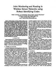
Figure 4 Sensor deployment in the Gaussian distribution. Here solid dots represent sensor nodes and hollow circles represent cluster heads. In this 50m × 50m target area , 40 sensor nodes are deployed and are divided into 4 groups, each group contains 3 cluster heads and 10 sensor nodes within the 25m × 25m targeted area. Within each sub region, the 10 sensor nodes and 3 cluster heads are distributed in Gaussian distribution with the central point of the sub region as mean point. The standard deviation sigma is set to σ = 25m/6. Under this setting, the probability that a sensor node is out of the sub region is less than 0.03%. The cluster heads are deployed randomly.


25

Lifetime of the Sensor Network

10000 Gaussian Distribution Uniform Distribution 9000

8000

7000

6000 5

6

7

8

9

10

11

12

13

14

15

Broadcast Rounds Figure 5 Rounds vs. lifetime for the uniform distribution and the Gaussian distribution. Here the network size is N = 40, and is divided into 4 groups, with each groups 10 nodes. The distribution of the nodes follows Fig. 4. The uniform distribution means within each group, the nodes are distributed in the targeted area with even probability.

26


8700 Gaussian Distribution Uniform Distribution

Lifetime of Sensor Network

8600 8500 8400 8300 8200 8100 8000 1

2

3

4

5

6

7

8

9

10

Exponent of Link Cost Metrics Figure 6 Exponent of link cost metrics β vs. network lifetime. Here the network size is N = 40, and is divided into 4 groups, with each groups 10 nodes. The distributions of the nodes will follow Fig. 4. The broadcast interval m is chosen to be 10. The key observation is that when β = 5, the lifetime reaches the maximum.


27

9000 Gaussian Distribution Uniform Distribution

Lifetime of Sensor Network

8000 7000 6000 5000 4000 3000 2000 1000 0 2.0

2.2

2.4

2.6

2.8

3.0

Exponent of Energy Equation Figure 7 Exponent of energy equation α vs. network lifetime. Here the network size is N = 40, and is divided into 4 groups, with each groups 10 nodes, the distribution of the nodes will follow Fig. 4. The broadcast interval m is chosen to be 10, and the exponent β is set as 10. When α changes from 2 to 3, the lifetime decreases dramatically.

28


Figure 8 Number of cluster heads vs. network lifetime. Here the network size is N = 60, and is divided into 6 groups, with each groups 10 nodes, the distribution of the nodes will follow Fig. 4. The broadcast interval m is chosen to be 12, and the exponent β is set as 10, α is set as 5. When the number of cluster heads changes from 1 to 5, the lifetime increases slightly.