13th World Conference on Earthquake Engineering Vancouver, B.C., Canada August 1-6, 2004 Paper No. 0959
GEOGRAPHICALLY DISTRIBUTED CONTINUOUS HYBRID SIMULATION Gilberto MOSQUEDA1, Bozidar STOJADINOVIC2 and Stephen A. MAHIN3
SUMMARY The hybrid simulation test method is a versatile technique for evaluating the seismic performance of structures by seamlessly integrating both physical and numerical simulations of substructures into a single test model. The use of geographically distributed substructures in a hybrid simulation allows for the evaluation of complex structural model by enabling simultaneous testing of multiple large-scale experimental substructures. To improve the reliability and efficiency of tests involving multiple experimental sites, a distributed control system is presented that supports the implementation of advanced continuous hybrid simulation algorithms. The controller is based on an event-driven scheme, instead of a real-time clock-based scheme, to implement continuous algorithms on distributed models where network communication, numerical integration and other tasks may have random completion times. The eventdriven controller uses logic to reduce the adverse effects of random task times, which can compromise the stability and accuracy of the test. The effectiveness of this procedure is demonstrated by computing the earthquake response of a two-story shear building model with two remote physical substructures connected using the Internet. INTRODUCTION Hybrid simulation is a method intended to evaluate the seismic performance of structures. The principles of the hybrid simulation test method are rooted in the pseudodynamic testing method developed over the past 30 years (Takanashi et al. [1], Takanashi and Nakashima [2], Mahin et al. [3], Shing et al. [4], Magonette and Negro [5]). In a hybrid simulation, the dynamic equation of motion is applied to a hybrid model, which includes both numerical and experimental substructures. Typically, the experimental substructures are portions of the structure that are difficult to model numerically, thus, their response is measured in a laboratory. Numerical substructures represent structural components with predictable behavior: they are modeled using a computer.
1
Post-Doctoral Researcher, Univ. of California, Berkeley, USA. Email:
[email protected] Associate Professor, Univ. of California, Berkeley, USA. Email:
[email protected] 3 Byron L. and Elvira E. Nishkian Professor of Structural Engineering, Univ. of California, Berkeley, USA. Email:
[email protected] 2
Hybrid simulation procedures have advanced considerably since the method was first developed. Early tests utilized a ramp-hold loading procedure on the experimental elements. Recently developed techniques along with advancements in computers and testing hardware have improved this test method through continuous tests at slow (Magonette [6]) and fast rates (Nakashima [7]). The potential of the hybrid simulation test method has been further extended by proposing to geographically distribute experimental substructures within a network of laboratories, then link them through numerical simulations using the internet (Campbell and Stojadinovic [8]). The infrastructure of the George E. Brown Jr. Network for Earthquake Engineering Simulation (NEES) provides the experimental equipment, the analytical modeling tools and the network interface to research complex analytical models with the simultaneous testing of multiple large-scale experimental substructures using the distributed hybrid simulation approach. Geographically distributed hybrid simulation has already been carried out jointly between Japan and Korea (Watanabe et al. [9]), in Taiwan (Tsai et al. [10]) and in the U.S. as part of the NEES efforts (MOST [11]). However, these applications of distributed hybrid simulation have used the ramp-hold procedure to load the experimental substructures. As such, they are not benefiting from the advanced continuous methods that can improve the measured behavior of the experimental substructures and the reliability of the test results. The difficulty in applying real-time based continuous algorithms to distributed applications stems from their lack of suitability with tasks that involve random completion times. Random completion times in network communication, numerical integration and other such tasks could compromise the stability of real-time algorithms because they may not complete in the time required by the real-time test clock. The ramp-hold loading procedure can be readily applied to deal with random delays since the hold period can be arbitrarily long. However, the ramp-hold procedure introduces a number of other errors. In order to maintain the benefits of continuous testing, an event-driven procedure is proposed for conducting continuous tests over a network that minimizes, if not eliminates, the hold phase at each integration step. A distributed hardware architecture utilizing event-driven controllers is also presented and verified experimentally. The experiments presented here are the first-ever attempt to conduct a continuous hybrid simulation distributed over multiple facilities that are linked through the internet. HYBRID SIMULATION TEST METHOD The equipment used for quasi-static testing in most structural testing facilities can also be utilized to conduct hybrid tests. The basic components of a pseudodynamic test setup and their interconnections are illustrated in block diagram form in Figure 1. The required tools are: (1) a servo-hydraulic system consisting of a controller, servo-valve, actuator and pressurized hydraulic oil supply; (2) a test specimen with the actuators attached at the point where the displacement degrees of freedom are to be imposed; (3) instrumentation to measure the response of the test specimen; and (4) an on-line computer capable of computing a command signal based on feedback from the transducers. The primary task of the on-line computer is to integrate the equation of motion utilizing the restoring force vector, ri, which is composed of forces from experimental and numerical substructures. A time-stepping integration procedure is used to solve the discretized equation of motion for displacement, d, velocity, v, and acceleration, a, at time intervals ti =i∆t for i=1 to N.
Mai + Cvi + ri = f i
(1)
The subscript i denotes the time-dependant variables at time ti, ∆t is the integration time step and N is the number of integration steps. The mass matrix, M, damping matrix, C, and applied loading, f, are typically
hydraulic supply
dc integrator signal generation
D/A
servo-valve actuator
PID
da = actual imposed displacement dc = command displacement dm = measured displacement rm = measured restoring force
Controller on-line computer servo-hydraulic system
dm rm
A/D
da
specimen transducers
A/D
experimental substructure
FIGURE 1. Block diagram of test setup modeled as part of the numerical simulation. Numerical methods used to solve the equation of motion are discussed in Mahin and Shing [12]. The same methods are extended to hybrid simulation. Continuous Testing Applying a continuous load history, rather than a ramp-hold load history, improves the measured behavior of the experimental substructure (Magonette [6]). The improvements are largely based on the elimination of the hold phase and the associated force relaxation in the experimental specimens. Continuous testing methods require a real-time platform to ensure the commands for the servo-hydraulic controller are updated at deterministic rates. Constant update rates allow for the control of the actuator velocity, thus allowing for a continuous load history (non-zero velocity) on the experimental elements. The difference between the ramp-hold and a continuous load history is shown for one simulation step in Figure 2. Note that the continuous procedure utilizing a predictor/corrector approach reduces the velocity demands for the same time interval. An example of a predictor/corrector technique for continuous loading is summarized below.
actuator command
In their algorithm for real-time testing, Nakashima and Masaoka [13] separate the computations in the online computer into two tasks running at different sampling rates: (1) the response analysis task, which carries out the integration of the equation of motion and 2) a signal generation task, which provides displacement commands to the servo-hydraulic actuator at a rate faster than that of the integration time step. These two tasks run on a Digital Signal Processor (DSP) in real-time using a multi-rate approach. The response analysis task deals with the typical numerical algorithms for solving the equation of motion. The signal generation task, on the other hand, computes the displacement path of the actuator using polynomial approximation procedures. Nakashima and Masaoka showed that third order polynomial
computation di+1
corrector predictor
di
application
ramp
computation
continuous ramp-hold
hold ∆Ti (simulation time step) actual time
FIGURE 2. Ramp-hold and continuous load history
interpolation and extrapolation of known displacement values from previous steps provide accurate displacement and velocity predictions in the current step. The key to this polynomial approximation procedure is that the computation time is small and actuator commands can be continuously generated at small constant time intervals. For each integration step, the actuator is kept in motion after achieving the target displacement by predicting a command signal based on polynomial extrapolation of the previous target displacement values. Meanwhile, the integrator task is carrying out computations for the next target displacement. Once the integration task has been completed and the target displacement is known, the controller switches to interpolate towards the correct target value. An advantageous feature of this algorithm is that the communication between the integration task and the signal generation task is minimized. DISTRIBUTED HARDWARE ARCHITECTURE
NETWORK
The typical architecture of a hybrid simulation controller consists of the integration loop commanding the inner servo-hydraulic controller loop as previously shown in Figure 1. A single processor is used to compute both the integration of the equation of motion and the signal generation of the actuator commands. The separation of these two tasks into different processors provides an expandable distributed architecture for simultaneous testing of multiple substructures as show in Figure 3. Moreover, increased processing time can be dedicated to the integrator task for applications with large numerical structural models. In a local testing configuration, the network is replaced by a shared memory bus (Systrans [14]) to maintain fast communication rates for real-time continuous algorithms. In the case of geographically distributed testing, Ethernet replaces the network link. As will be demonstrated in the discussion of the experimental results, network communication time is random, and therefore not suitable for real-time algorithms. A solution based on a finite-state event-driven controller design is discussed next.
dm DSP Signal Generation
dij+1
PID Servo-hydraulic control
rm
Actuator Load cell
PC Integrator Algorithm
Remote Substructure A
Analysis Site
dm DSP Signal Generation
dij+1
PID Servo-hydraulic control
rm
Actuator Load cell
Remote Substructure B
FIGURE 3. Distributed hardware architecture for geographically distributed testing
EVENT-DRIVEN SIMULATION In cases where task execution times are random, a clock-based control scheme could fail if the required processes are not completed within the allotted time. As an improved alternative to the clock-based scheme used for real-time applications, an event-driven reactive system, based on the concept of finite state machines (Harel [15]) is proposed that responds to events based on the state of the hybrid simulation system. The event-driven system can be programmed to account for the complexity and randomness of real systems and, thus, take action to minimize the random effects on experimental substructures. The programming procedure is based on defining a number of states in which the controller can exist in and the transitions between these states that take place as specified events occur. Nakashima and Masaoka's [13] algorithm reacts to events in the sense that the algorithm switches from extrapolation to interpolation after the integration task is completed. However, the variance in task completion times for their application was minimal. They used an explicit integration method and the DSP running these tasks had a dedicated and reliable connection to the servo-hydraulic controller. This algorithm will not function effectively for distributed hybrid simulations involving the internet since random delays are likely to occur. The state transition diagram in Figure 4 shows the implementation of an event-driven version of a polynomial predictor/corrector command generation method. This algorithm continuously updates the actuator commands using the same approach under normal operation conditions and takes action for excessive delays. This diagram consists of five states: extrapolate, interpolate, slow, hold and free_vibration. The default state is extrapolate, during which the controller commands are predicted based on previously computed displacements while the integrator computes the next target displacement. The state changes from extrapolate to interpolate after the controller receives the next target displacement and generates the event D_update. The event D_target is generated once the physical substructure has realized this target displacement. The model then subsequently transitions back to the extrapolate state and sends updated measurements to the integrator. The smooth execution of this procedure is dependent on having a reliable network connection and selecting the run time of each integration step sufficiently large for all of the required tasks to finish. Small variations in completion times for these tasks will only affect the total number of extrapolation steps versus interpolation steps.
D_target extrapolate
D_update
interpolate free_vibration
TimeOut
D_update
D_update TimeOut
slow
TimeOut
hold
Legend State: State Transition Path: Event causing State Transition: Event/functionCall()
FIGURE 4. Event-driven scheme using a polynomial predictor/corrector to continuously generate actuator commands
The advantage of the event-driven approach is that logic can be included to handle excessive delays. For example, if the system is in the extrapolate state longer than a specified time, the actuator can deviate from the intended trajectory or even exceed its target, hence limits need to be placed on the number of allowable extrapolation steps. A simple solution is to generate the event TimeOut, which will transition the controller to the slow state. In the slow state, extrapolation continues at a reduced velocity to keep the actuator in continuous motion while allowing more time to receive an update. Upon receiving the next target displacement, the interpolate state is activated. If the update is not received within a set amount of time, the slow state needs to TimeOut as well, to place the actuator on hold until the target displacement is received. Longer delays, possibly due to the integrator crashing or a network failure, could indefinitely delay the controller receiving an updated displacement. For this rare event, the hold state can also time out and force the system into free_vibration or any other desirable state to dissipate the energy in the physical specimens and end the test. The free_vibration state is intended to fully unload the physical substructure based on locally stored mass and damping ratio for the test specimen. EXPERIMENTAL PROGRAM The hybrid simulation control system for geographically distributed testing is experimentally verified through tests conducted with substructures located at the UC Berkeley Campus and the Structural Engineering Laboratory at the Richmond Field Station. These two locations are approximately 5 miles apart, but they are connected through the UC Berkeley Ethernet network. The numerical analysis for a structural model is carried out on a computer located on Campus and is linked to two independent experimental substructures located at the Richmond Field Station Structural Engineering Laboratory using Ethernet and TCP/IP. The event-driven distributed control architecture is implemented to manage the random communication delays between these two sites. The structural model consists of an idealized two-degree of freedom shear frame with two experimental substructures representing the column behavior. The frame is assumed to deform in pure shear with rigid beams as shown in Figure 5a. The columns have a point of inflection at mid-height of the story under the assumed deformation constraints, allowing for the extraction of two simple experimental substructures. The resisting shear forces for each story can be obtained experimentally by testing half of a column configured as a cantilever transversely loaded by an actuator. The other column in each story is assumed to behave the same as the tested column. The two identical cantilever test specimens in Figure 5b are used to model the two substructure columns on the first and second story. Preliminary characterization tests of the physical column models reveal that the initial stiffness is approximately 2.8 kip/in. Based on the m2=0.01 kip-s2/in.
m1=0.01 kip-s2/in.
a. structural model
d2
d1
b. test setup
FIGURE 5. Two-story shear frame with two experimental substructures
properties of the experimental elements and the mass assigned to the shear frame in Figure 5a, the resulting vibration periods of the structure are 0.62 seconds and 0.24 seconds for the first and second mode, respectively. The damping matrix is specified as stiffness proportional with 5 percent of critical damping in the first mode to quickly decay the transient response of the structure. The equation of motion for the structural model is solved using Newmark's [16] explicit integration algorithm implemented for hybrid testing (Mahin and Shing [12]). This algorithm was selected because it is simple to implement and its stability limits are suitable for the structural model under consideration. The appropriate geometric transformations are included in the numerical procedure to convert the global degrees of freedom shown in Figure 5a to the actuator degrees of freedom. The combined experimental and analytical structural model was subjected to the 1978 Tabas historical earthquake acceleration record with a length scale of 3 (time scale of 3 ). The amplitude scale was modified to a peak-ground acceleration (PGA) of 0.378g for an elastic level simulation (Tabas-50%) and to a PGA of 1.133g to obtain a non-linear response from the experimental substructures (Tabas-150%). Both earthquake simulations were allowed to run for 30 seconds using an integration time step of 0.01 seconds for a total of 3000 steps. The extended time scale for the slow continuous test was selected to accommodate about 95 percent of the simulation steps without having to slow down or hold the actuators. The time scale factor from the integration time step, ∆t, to the expected duration of each step was determined as follows. First, the TimeOut event triggers were determined based on the percentage of the command generation sub-step between the last target displacement, di, and the next target value di+1. The extrapolate state was allowed to predict the actuator trajectory path up to 60 percent of the step and the slow state was allowed to extrapolate up to 80 percent of the step. This procedure guaranteed that at least the last 20 percent of the command generation sub-steps were computed using the more accurate polynomial interpolation procedure. The free_vibration state was not implemented in these tests. Using preliminary test data to characterize the behavior of the network, it was estimated that about 95 percent of the steps could complete the integration task and the network communication task within 0.7 seconds. Based on these results and the goal to achieve 95 percent of the steps without delays, each integration step was scaled from 0.01 to 1.2 seconds, but a step would take longer if the network communication was delayed. As a result, the duration of the extrapolate portion of the command generation was allotted up to 0.72 seconds. This extended time scale reduced the actuator velocity in the extrapolate state by a factor of 120 compared to a real-time simulation. In the slow state, this velocity was halved, making the total duration of the slow state equal to 0.48 seconds while predicting up to 80 percent of the command generation sub-steps. If the delay in receiving the target displacement was greater than 1.2 seconds, the controller switched to the hold state and the actuator velocity went to zero. The interpolate state was activated for the remainder of the steps after receiving updated data. Within the event-driven scheme, the displacement commands were modified to compensate for the measured response lag in the actuators using the feed-forward procedure recommended by Horiuchi et al. [17]. EXPERIMENTAL RESULTS The experimental results from the distributed network hybrid simulations are presented and evaluated by a comparison to a pure numerical simulation. The exact same structural model and numerical algorithms are used in both the hybrid simulations and the pure numerical simulations. The main difference is that experimental elements are used in the hybrid simulation, which can include measurement errors and actuator tracking errors. In the numerical simulation, the experimental elements are replaced by numerical models calibrated using the measured force and measured displacement data from the corresponding
Second story drift (in.)
1 Hybrid Numerical
0.5 0 −0.5 −1
0
5
10
15 Time (sec.)
20
25
30
20
25
30
a. second story drift
First story drift (in.)
1 0.5 0 −0.5 −1
0
5
10
15 Time (sec.)
b. first story drift FIGURE 6. Computed response of two-story shear frame in the Tabas-50% simulation experiment. These numerical elements are "exact" in the sense that they do not contain experimental and tracking errors, thus, their numerical error is considered negligible. The Tabas-50% hybrid and pure numerical simulations were conducted first. The results are shown in Figure 6. Note that the ground motion amplitude in these simulations was scaled such that the structure remains elastic. A direct comparison of the distributed hybrid simulation and the numerical simulation displacement histories verifies that the distributed controller functions effectively in the presences of random network delays. In the hybrid simulation, the experimental substructure response is linear with calibrated stiffness values of 2.80 kip/in. for the first story and 2.82 kip/in. for the second story. Linear spring models with these stiffness values are used to compute the substructure resisting forces for the numerical simulation. The strong correlation between the two simulations indicates that experimental errors had a negligible effect on the hybrid simulation results. The Tabas-150% hybrid and pure numerical simulations were conducted next. The results are shown in Figure 7. Note that the ground motion amplitude in these simulations was scaled such that the columns respond in the inelastic range. The experimental results correlate well with the numerical simulation, particularly at the second story level. The maximum drift error between the two simulations occurs at the first story level and is 10 percent of the absolute maximum drift. In the hybrid simulation, the response of the second story substructure is linear, but the first story substructure behavior is non-linear. Accordingly, a linear spring model replaces the second story substructure and the non-linear Bouc-Wen model (Bouc [18], Wen [19]) replaces the first story substructure in the purely numerical simulation. As seen by comparing the experimental and analytical results in Figures 7c and 7d, respectively, the Bouc-Wen model captures the principal characteristics of nonlinear response very well. The negative peaks forces are
similar for both simulations, but the Bouc-Wen model predicts a larger positive peak force. The positive peak force is smaller for the experimental element because its strength degrades after yielding, while the strength of the numerical model does not degrade. Nonetheless, the numerical simulation and the hybrid simulation provide similar results.
Second story drift (in.)
4
Hybrid Numerical
2 0 −2 −4 0
5
10
15 Time (sec.)
20
25
30
20
25
30
a. second story drift
First story drift (in.)
4 2 0 −2 −4 0
5
10
15 Time (sec.)
b. first story drift 4
First story shear (kip)
First story shear (kip)
4 2 0 −2 −4
−4
−2 0 2 First story drift (in.)
c. measured response
4
2 0 −2 −4
−4
−2 0 2 First story drift (in.)
4
d. numerical simulation
FIGURE 7. Computed response of two-story shear frame in the Tabas-150% simulation
Test
No. of steps
Tabas-50% Tabas-150%
3000 3000
TABLE 1. Timing data summary Max. delay Total run (sec.) time (sec.) 6.59 5.9
% delayed steps Slow state 12.4 5.9
3667 3638
Hold state 1.7 0.9
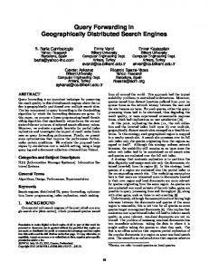
Performance of Event-Driven Controller During the network tests, there were several instances when the event-driven controller did not receive data from the integrator during the 0.72-second long extrapolation state and activated the slow and then hold states. Figure 8 shows the distribution of the time taken for the local DPS to receive data from the integrator after passing a target displacement. The time captured is the integration task time and the network communication time measured during the Tabas-50% simulation. The dashed lines in the figure represent the limits where the slow and hold states are activated according to the selected simulation timing scheme. Table 1 provides a summary of the network delay statistics including: the maximum delay, the total run time for the test and the percentage of the steps in which the slow and hold states were activated. It is interesting to note that the test with the most delays (Tabas-50%) overran the total target simulation time of 3600 seconds by only 67 seconds. More importantly, the actuators subjected the experimental specimens to a hold phase for less than two percent of the simulation steps. The simulation Tabas-150% has less than half of the delayed steps compared to Tabas-50%. The variation of delays between the two simulations is characteristic of the network behavior and is likely due to variations in network congestion during the time the test was executed. Effects of Delays on Experimental Substructures Figure 9 provides a close look at the behavior of the yielded first-story substructure during the Tabas150% simulation for steps that experienced delays. The data in the figure concentrates on 20 seconds of simulation time, corresponding to 10 integration time steps. The time scale shown in the figure corresponds the DSP clock time and not the simulation earthquake time. The state of the event-driven algorithm is shown in Fig 9a. The Y-axis marks the (E)xtrapolate, (I)nterpolate, (S)low and (H)old states. As indicated in Figure 9a, the first few steps executed smoothly by switching directly from extrapolate to interpolate. At approximately 1875 seconds into the test, two short delays occurred followed by two longer delays. The length of the delays are identified by the amount of time spent in the (H)old state. The measured displacement history and force history are show for the same 20 seconds of DSP clock time in
No. of steps
150 SLOW STATE
100
HOLD STATE
50
0
0
0.5
1
1.5 Step duration (sec.)
2
2.5
3
FIGURE 8. Histogram of target displacement update time during the Tabas-50% simulation
0.5
Measured displ. (in.)
H
State
S
I
E 1780
1785
1790 1795 Time (sec.)
0.45 0.4 0.35 0.3 1780
1800
−1.05
−1.1
−1.1
−1.15 −1.2 −1.25 −1.3 −1.35 1780
1785
1790 1795 Time (sec.)
1800
b. measured displacement
−1.05
Measured force (kip)
Measured force (kip)
a. state
1785
1790 1795 Time (sec.)
1800
−1.15 −1.2 −1.25 −1.3 −1.35 0.3
0.35 0.4 0.45 Measured displ. (in.)
0.5
c. measured force d. hysteresis FIGURE 9. Behavior of experimental substructure during the hold state in the Tabas-150% simulation Figure 9b and Figure 9c, respectively. The measured force history and the force-displacement data in Figure 9d illustrate the consequences of a hold phase on the behavior of the experimental substructures. During the hold period, the displacement remains constant as expected, but the force decreases in magnitude. The corresponding segment of the hysteresis provides further evidence of force relaxation, particularly during the two long delays. The circular markers on subplots a-d indicate the end of the simulation step where measurements are taken for a step with a 0.2 seconds hold period. In this case, there is negligible force relaxation and sufficiently accurate measurements are obtained. The 'x' marker notes the end of the step with a much longer delay, resulting in a 4.7 seconds hold phase. Note from the force displacement data in Figure 9d that the measured force value is taken while the specimen is recovering from force relaxation. Consequently, the measured force used in the integration algorithm is in error. Steps in which the hold state is not activated provide a smooth force-displacement response, including the delayed steps in which the specimen is only subjected to the slow state because the actuator kept moving continuously without stopping. CONCLUSIONS A versatile controller for continuous hybrid simulation with capabilities for geographically distributed testing was presented. The randomness associated with internet communication was handled by an eventdriven distributed control system, which provided a fault-tolerant mechanism to handle random delays and minimize force relaxation and rate-related errors in the experimental substructures. The proposed system
was experimentally verified through hybrid simulations of a two-degree of freedom structural model with two remote experimental substructures connected using the internet. An evaluation of the test data confirms that the distributed testing procedure provides reliable results. The experimental studies described in this report represent the first-ever geographically distributed hybrid simulations using continuous algorithms. The feasibility of distributed testing using advanced algorithms and the reliability of the hybrid simulation results were confirmed. These tests also demonstrate the potential of the hybrid simulation test method to evaluate the seismic performance of complex structural models by the simultaneous testing of multiple substructures in remote facilities. The distributed experiments presented here were conducted within facilities relatively close to each other. Longer and more frequent network delays are expected to occur for tests involving more distant sites. The distributed control strategy is applicable to such tests, although it might be necessary to further extend the simulation time scale in order to minimize the occurrences of hold periods. To improve the performance of this testing method to longer and more frequent delays, predictor/corrector schemes that can accurately predict the actuator path beyond one integration time step are needed. ACKNOWLEDGMENTS This research was supported by the National Science Foundation through the UC Berkeley NEES equipment site grant CMS-0086621. Their support is gratefully acknowledged. Graduate student Mr. Andreas Shellenberg assisted in running the experiments. Mr. Don Clyde and Mr. Wes Neighbor provided generous support during the experimental setup and testing. REFERENCES 1.
2. 3. 4. 5. 6.
7.
8.
9.
Takanashi, K., Udagawa,K., Seki, M., Okada, T. and Tanaka, H. “Non-linear earthquake response analysis of structures by a computer-actuator on-line system (details of the system).” English translation of paper in: Transactions of the Architectural Institute of Japan March 1975, 229:77-83. Takanashi, K. and Nakashima, M. “Japanese activities on on-line testing.” Journal of Engineering Mechanics 1987, 113(7):1014-1032. Mahin S.A., Shing, P.B., Thewalt, C.R. and Hanson, R.D. “Pseudodynamic test method - Current status and future direction.” Journal of Structural Engineering 1989, 115(8):2113-2128. Shing, P.B., Nakashima, M. and Bursi, O.S. “Application of pseudodynamic test method to structural research.” Earthquake Spectra 1996, 12(1): 29-54. Magonette, G.E. and Negro, P. “Verification of the pseudodynamic test method.” European Earthquake Engineering 1998, XII(1):40-50. Magonette, G. “Development and application of large-scale continuous pseudo-dynamic testing techniques.” Philosophical Transactions of the Royal Society: Mathematical, Physical and Engineering Sciences 2001, 359:1771-1799. Nakashima, M. “Development, potential, and limitations of real-time online (pseudo-dynamic) testing.” Philosophical Transactions of the Royal Society: Mathematical, Physical and Engineering Sciences 2001, 359:1851-1867. Campbell, S. and Stojadinovic, B. “A system for simultaneous pseudodynamic testing of multiple substructures.” Proceedings, Sixth U.S. National Conference on Earthquake Engineering, June 1998. Watanabe, E., Kitada, T., Kunitomo, S. and Nagata, K. “Parallel pseudo-dynamic seismic loading test on elevated bridge system through the Internet.” The Eight East Asia-Pacific Conference on Structural Engineering and Construction, Singapore, December 2001.
10.
11. 12. 13. 14. 15. 16. 17.
18. 19.
Tsai, K.-C., Yeh, C.-C., Yang, Y.-S., Wang, K.-J., Wang, S.-J. and Chen, P.-C. “Seismic Hazard Mitigation: Internet-based hybrid testing framework and examples.” International Colloquium on Natural Hazard Mitigation: Methods and Applications, France, May 2003. MOST. Multi-site On-line Simulation Test. NEESgrid 2003, http://www.neesgrid.org/most/. Mahin S.A. and Shing, P.B. “Pseudodynamic method for seismic testing.” Journal of Structural Engineering 1985, 111(7):1482-1503. Nakashima M. and Masaoka, N. “Real-time on-line test for MDOF systems.” Earthquake Engineering and Structural Dynamics 1999, 28(4):393-420. Systran. SCRAMNet+ Network. Systran Corporation 2003. Harel. D. “Statecharts: A visual formalism for complex systems.” Science of Computer Programming 1987, 8:231-274. Newmark, N.M. “A method of computation for structural dynamics.” Journal of Engineering Mechanics 1959, 85(3):67-94. Horiuchi, T., Inoue, M., Konno, T. and Namita. Y. “Real-time hybrid experimental system with actuator delay compensation and its application to a piping system with energy absorber.” Earthquake Engineering and Structural Dynamics 1999, 28(10):1121-1141. Bouc, R. “Modèl mathématique d’hysteresis.” Acustica 1971, 24:16-25. Wen, Y.-K. “Method for random vibration of hysteretic systems.” Journal of Engineering Mechanics 1976, 102(2):249-263.