geometric primitive feature extraction – concepts ...

GEOMETRIC PRIMITIVE FEATURE EXTRACTION – CONCEPTS, ALGORITHMS, AND APPLICATIONS

DILIP KUMAR PRASAD

School of Computer Engineering

A Thesis submitted to the Nanyang Technological University in fulfillment of the requirement for the degree of Doctor of Philosophy

2012

Abstract

This thesis presents important insights and concepts related to the topic of the extraction of geometric primitives from the edge contours of digital images. Three specific problems related to this topic have been studied, viz., polygonal approximation of digital curves, tangent estimation of digital curves, and ellipse fitting anddetection from digital curves. For the problem of polygonal approximation, two fundamental problems have been addressed. First, the nature of the performance evaluation metrics in relation to the local and global fitting characteristics has been studied. Second, an explicit error bound of the error introduced by digitizing a continuous line segment has been derived and used to propose a generic non-heuristic parameter independent framework which can be used in several dominant point detection methods. For the problem of tangent estimation for digital curves, a simple method of tangent estimation has been proposed. It is shown that the method has a definite upper bound of the error for conic digital curves. It has been shown that the method performs better than almost all (seventy two) existing tangent estimation methods for conic as well as several non-conic digital curves. For the problem of fitting ellipses on digital curves, a geometric distance minimization model has been considered. An unconstrained, linear, noniterative, and numerically stable ellipse fitting method has been proposed and it has been shown that the proposed method has better selectivity for elliptic digital curves (high true positive and low false positive) as compared to several other ellipse fitting methods. For the problem of detecting ellipses in a set of digital curves, several innovative and fast preprocessing, grouping, and hypotheses evaluation concepts applicable for digital curves have been proposed and combined to form an ellipse detection method. Performance of the proposed ellipse detection method is better than several recent ellipse detection methods and close to the ideal case. All algorithms presented in this thesis have been developed using detailed mathematical analysis of the discrete geometry involved. The validity of these methods has been verified using rigorous mathematical analysis, numerical experiments in various difficult scenario, and extensive testing on large image datasets of practical importance. The utility of these algorithms has been shown using three practical applications related to image processing for robotics, medical image processing, and object and face detection.

i

Acknowledgements

कमर्णयेवािधकार ते मा फलेषु कदाचन।

मा कमर्फलहे तभ ु म ूर् ार् ते सङ्गोऽ

वकमर्िण।

“Yours is the right to perform, not the right to expect (the fruits of your actions). Do not let the fruit be the purpose of your actions. By being driven by the fruits of your actions, do not lead yourself to inaction.” -Bhagvad Gita (Chapter 2.47)

In this proud moment of my life, when I am writing the acknowledgement for my PhD dissertation, I pay my respects first to all the wise people in my life like my parents, my teachers, and the Bhagvad Gita for reiterating the above quote time and again in my life. I pay my humble respects to my teachers. Specifically, I recall the teachers who left indelible marks in my life: my parents, my elder sister Kaushalya, Master Ji, Ratan Maharaj (little monk) from Ramakrishna Ashram, Mrs. Gopa Gupta, Mrs. Tapati Das, Mrs. S. Mukherjee, Mr. Lal Bahadur Shastri, Dr. Subrata Bose, Mr. Arup Pal, Dr. Munindra Prakash, Dr. A Chattopadhayay, Dr. D.P Mukherjee, Dr. Maylor K.H. Leung, Dr. Janusz Starzyk, Dr. Wendy Torrance, and Dr. Chai Quek (in the chronological order of their first impact in my life). Life is a great teacher, and I salute to the provider of life and my little Ganesha. I especially thank Mrs. Gopa Gupta, Dr. Subrata Bose, Mr. Girish Mishra, Dr. Janusz Starzyk, Dr. Wendy Torrance, Dr. Maylor Leung, and Dr. Chai Quek, for mentoring a vagabond and stubborn person as me. I am very grateful to Dr. Maylor Leung for giving me the independence to pursue independent research on the topic of discrete geometry and for scrutinizing several lengthy derivations very patiently and persistently. I respect his philosophy of never compromising on the quality of work and this has motivated me to keep high expectation from myself in terms of the quality of work. I take this opportunity to thank Nanyang Technological University and Ministry of Education, Singapore for providing me with the necessary infrastructure and funding for my doctoral studies. I thank Dr. Jiang Xudong, Dr. Chai Quek, Dr. Wolfgang Mueller, Dr. Janusz Starzyk, Dr. Philip Fu, and Dr. Mao Kezhi for conducting exceptional graduate modules. I thank Centre of Life Sciences, National University of Singapore for allowing me to fulfill my

ii

desire to acquire more knowledge about the field of Neuroscience. I thank Dr. Dale Purves, Dr. George Augustine, Dr. Shih-Cheng Yen, Dr. Thorsten Wohland, Dr. Ji Hui,Dr. Soong Tuck Wah, Dr. Antonius VanDongen, Dr. Marc Fivaz, Dr. Hongyan Wang, Dr. Fengwei Yu, Dr. Eyleen Goh, and Dr. Suresh Jesuthasan for conducting the post graduate modules on Vision and Perception, Neuronal Signaling, Developmental Neurobiology and Neurological and Behavioural Disorder and making me an active participant of these modules. I thank Dr. Janusz Starzyk and Dr. Krishna Agarwal for being a constant source of inspiration for me. I thank Dr. Siu-Yeung Cho and Mrs. Christina Lee for providing me with a good and hasslefree laboratory environment. I had the privilege of having great friends in my life, who make the life a rich and happy experience. I begin with the friends who helped me directly or indirectly with my doctoral studies. I thank Dr. Krishna Agarwal for motivating and helping me to join the doctoral program. I thank Dr. Raj Gupta, Deepak Subramanian, Dr. Ashis Mallick, and Dr. Ranjan Das for being and remaining very good friends in odd and even times. Other friends in my research lab, who deserve special mention, are Dr. Tang Chaoying, Dr. Hengyi Zhang, Dr. Atiqur Rahman, Dr. Pravin Kakar, and Ha Thanh. My Ph.D. life would not have been as much fun without Melanie, Sulley Goh, Ngyuen Chi, Dr. Balaji Gokulan, Dr. Dwarikanath Mohapatra, Mimi, Kabita bhabhi, and fellow ISMites (Abhishek Seth, Dr. Amit Sachan, Dr. Amit Singh, Arpita Singh, Kushal Anand, Dr. A.V. Subramanyam, Dr. Alok Prakash, and Neha Tripathi) in Singapore. I also thank my friends and ex-colleagues, who are too many to count. In a non-exclusive list, I mention Vijay, Abhishek Awasthi, Srikanth, Pillai, Sridhar, Ramesh Babu, Atul Jha, Chandrashekar, Vineet Singh, Himanshu Pati, Kambli, Ashu, Dubi, and Kuseswar Prasad. I recall fondly Sanju, Sunita, Nupur, Loet, Erik, David Gernaat, Leila, and others. My start-up team Bharti, Prashant, Dishant, and Mohit Bansal understood my commitment towards my thesis and supported me throughout last 2 years. I am thankful to them too. I thank the 20 volunteers who participated in the generation of ground truth for section 6.1. They are Dr. A.V. Subramanyam, Dr. Alok Prakash, Dr. Amit Sachan, Dr. Amit Singh, Dr. Atiqur Rahman, Dr. Balaji Gokulan, Dr. Dwarikanath Mohapatra, Dr. Hengyi Zhang, Dr. Krishna Agarwal, Dr. Raj Kumar Gupta, Abhishek Seth, Deepak Subramanian, Kushal Anand, Neha Tripathi, Ngyuen Chi, K. Prasad Sir, Dr. Manish Narwaria, Bharti, Prashant, and Dishant. iii

I acknowledge the support received from Dr. Alex Chia during my first month of Ph.D. and providing me with his insight about the problem of ellipse detection and sharing his source code for generating synthetic data for ellipse detection experiment. I acknowledge Dr. P. Kovesi, Dr. F. Mai, Dr. A. Opelt, Dr. R McLaughlin, Dr. Partha Bhowmick, and Dr. J.-O. Lachaud for sharing their insights or source code or executables for generating the results of their methods. I convey love and gratitude to my sisters, Kaushalya and Sangita for keeping me on track of my studies right from childhood. I would like to give special thanks to each and every person of my neighborhood during my childhood who indirectly took special care of me by protecting me from all the evil things and negative influences around me. I would like to thank my best friend Bhaskar and teenage friends Deepak, Narayan, Sulendra, Rajendra, Subodh, Mantu, Pintu, Bablu, Shankar da, Dadu, and others for protecting me from wrong and dark career paths. I like to thank Deepika for being indirect source of inspiration to study harder during senior school days. I thank Kaushalya Gupta and Sangita Gupta for taking care of my family in the difficult times and ensuring that my parents do not miss my presence. I fall short of words when trying to acknowledge my loving wife, Krishna. She has excelled and helped me in every possible way to pursue my study. I dedicate this important document of my life to my family and everyone related to me directly or indirectly in my life. My achievements are collective efforts of each and everyone in my life. I hope that this thesis will inspire a few future researchers to understand and tap the potential of discrete geometry in image processing applications.

Dilip Prasad

iv

Tablee of conntents

Abstracct ............................................................................................................................................ i  Acknow wledgementts .........................................................................................................................ii  Table oof contents ............................................................................................................................. v  Table oof figures .............................................................................................................................. xi  List of ttables.................................................................................................................................. xv  List of aabbreviationns .................................................................................................................... xvi  Chapterr 1 : Introduuction .................................................................................................................. 1  1.1 B Background ........................................................................................................................... 1  1.2 Polygonal ap pproximatioon of digitall curves ......................................................................... 6  Tangent estim mation for digital d curvees .................................................................................. 8  1.3 T 1.4 Primitive elliipse fitting ................... . .................................................................................... 11  1.5 E Ellipse detecction for praactical scenaario using hybrid h approoach....................................... 13  1.6 Practical appplications........................................................................................................... 18  Research nott covered inn the thesis ................... . ................................................................. 19  1.7 R 1.8 O Outline and highlights h o the thesis ................................................................................... 19  of Chapterr 2 : Polygoonal approxiimation of digital d curvees ............................................................. 25  2.1 B Background ......................................................................................................................... 25  2.11.1 Performaance metriccs .................................................................................................... 25  2.11.2 Control parameter p a optimization goal ................................................................... 26  and 2.11.3 Experim ments for PA A methods ....................................................................................... 27  2.11.4 : Outlinee and major contributio ons ............................................................................... 28  2.2 L Local and global qualities of fit.......................................................................................... 29  2.22.1 Precisionn and reliabbility metriccs ................................................................................. 29  v

2.22.2 Duality of o precisionn and reliabiility ............................................................................. 30  2.22.3 Existing performancce metric inn the contexxt of precisio on and reliaability ................. 34  2.22.4 Generaliizing precisiion and reliiability metrrics for dataasets ...................................... 35  2.3 A Algorithm baased upon precision p annd reliabilityy optimizatiion (PRO) ............................. 37  2.33.1 Precisionn and Reliabbility basedd Optimizatiion (PRO) ................................................ 38  2.33.2 Numericcal examples .................................................................................................... 39  2.4 C Continuous and a digital lines l – errorr bound duee to digitizattion ....................................... 49  2.44.1 Error bound of the slope s due too digitization .............................................................. 49  2.44.2 Error bound of maxximum deviaation and noon-parametrric framewoork for PA .......... 51  2.44.3 Compariison with otther boundss ................................................................................... 53  2.5 A Algorithms with w non-paarametric fraamework foor PA ........................................................ 58  2.55.1 Ramer-D Douglas-Peuucker’s metthod ............................................................................. 58  2.55.2 Masood’’s method ......................................................................................................... 66  2.55.3 Carmonaa’s method ................... . .................................................................................... 77  2.6 E Existing PA methods inn the contextt of precisioon, reliabilitty, and the error e boundd ........ 87  2.66.1 Optimal polygonal representati r ion of Perezz and Vidal [52] ...................................... 87  2.66.2 Ramer-D Douglas-Peuucker [12, 13] 1 (RDP annd RDP-mood).......................................... 88  2.66.3 Lowe’s method m [53]..................................................................................................... 88  2.66.4 Precisionn and reliabbility based optimizatioon (PRO) .................................................. 89  2.66.5 Break po oint suppresssion methood of Masoood [46] (Maasood and Masood-mod M d) ...... 89  2.66.6 Method of Carmonaa-Poyato [35] (Carmonna and Carm mona-mod) .................. . ......... 89  2.66.7 Nguyen and Debledd-Rennessonn’s PA methhod based on o blurred seegments ............. 90  2.7 Innteresting properties – comparison n among prooposed algo orithms .................................. 90  2.77.1 Experim ment 1 – scalling of digittal curves annd impact on o PA .................................... 90  2.77.2 Experim ment 2 – noissy digital cuurves ........................................................................... 96  2.77.3 Experim ment 3 – nonn-digitized and a semi-diggitized curvves ......................................... 99  2.77.4 Experim ment 4 – Perfformance ov ver datasetss ............................................................. 102  vi

2.77.5 Recomm mendations ................... . .................................................................................. 105  2.8 C Conclusion ......................................................................................................................... 105  Chapterr 3 : Tangennt estimationn of digital curves ...................................................................... 107  3.1 B Background ....................................................................................................................... 107  3.2 E Example of importance i of tangent estimation e ................................................................. 108  3.22.1 Yuen’s three t point method m [28]] for findingg the centerrs of the elliipses ................. 108  3.22.2 Error meetric and tanngent tests .................................................................................... 109  3.3 D Definite erroor bounded (DEB) ( tanggent estimatiion ......................................................... 113  3.33.1 Algorithhm.................................................................................................................... 113  3.33.2 Computaation compllexity ........................................................................................... 115  3.4 E Error bound of the proposed tangennt estimatorr for conic curves c .................................. 116  3.44.1 Analyticcal error bouund ............................................................................................... 116  3.44.2 Total errror bound inncluding thee effect of digitization d . ................... ......................... 118  3.44.3 Control parameter p R and multig grid perform mance .................................................... 119  3.5 N Numerical ex xamples to illustrate thhe error bounnd .......................................................... 122  3.6 C Comparison of DEB witth other tan ngent estimaators ....................................................... 126  3.66.1 Algorithhms used forr comparisoon .............................................................................. 126  3.66.2 Setup for comparisoon ................................................................................................. 128  3.66.3 Experim ment with cirrcular geom metry .......................................................................... 129  3.66.4 Experim ment with ellliptic geomeetry ........................................................................... 131  3.66.5 Experim ment with noon-conic shaapes containning inflexioon points ............................. 133  3.7 C Conclusion ......................................................................................................................... 135  Chapterr 4 : Least squares s fittinng of ellipsees .............................................................................. 137  4.1 B Background ....................................................................................................................... 137  4.2 A Algebraic disstance miniimization annd Fitzgibboon’s methodd .......................................... 140  4.22.1 Introducction to the method m ........................................................................................ 140  4.22.2 Numericcally stable algebraic fiitting (NSAF F)........................................................... 141  vii

4.3 G Geometric diistance minnimization..................................................................................... 142  4.4 G Geometry baased least sqquares fittinng of ellipsees - ElliFit ............................................... 144  4.44.1 Modificaation of the minimizatiion functionn ............................................................. 144  4.44.2 Mathematical modeel of ElliFit ................... . ............................................................... 145  4.44.3 Uniquenness of non-linear operaator ........................................................................... 147  4.44.4 Numericcal stability of linear opperator ....................................................................... 150  4.44.5 Algorithhm and compputational complexity c ................................................................ 152  4.5 C Comparison with other methods m ...................................................................................... 153  4.55.1 Digital inncomplete or o completee elliptic currves ........................................................ 154  4.55.2 Noisy cluster of poiints around an ellipse.................................................................. 158  4.55.3 Multiplee incompletee ellipses within w an imaage ......................................................... 163  4.55.4 Non-ellip ptic conics – analyticall and digitall ............................................................. 167  4.55.5 Non-ellip ptic noisy conics c ........................................................................................... 169  4.6 C Conclusion ......................................................................................................................... 173  Chapterr 5 : Ellipsee detection method m ......................................................................................... 175  5.1 B Background ....................................................................................................................... 175  5.2 Inntroduction and noveltyy of the ECC ellipse deetector .................................................... 176  5.3 Pre-processinng – obtainiing edge coontours of sm mooth curvaature ................................... 179  5.33.1 Sharp tuurns detectioon ................................................................................................. 180  5.33.2 Inflexion n points detection .......................................................................................... 181  5.4 G Grouping and elliptic hyypotheses ev valuation .................................................................. 183  5.44.1 Search reegion and edge e contouurs inside it ................................................................ 183  5.44.2 Associatted convexitty of the eddge contourss inside the search regioon .................... 184  5.44.3 Detection of the geoometric cennters of EH ................................................................ 186  5.44.4 Determinnation of thhe relationsh hip score.................................................................... 187  5.44.5 Grouping and hypottheses evaluuation ........................................................................ 190  5.5 Saliency andd elliptic hyppotheses sellection ...................................................................... 191  viii

5.55.1 Detection of similarr ellipses ...................................................................................... 191  5.55.2 Computaation of threee saliency criteria...................................................................... 192  5.55.3 Determinnation of thhe net salienncy score ................................................................... 194  5.55.4 The prop posed schem me for hypootheses selecction ....................................................... 199  5.6 N Numerical ev valuation ........................................................................................................ 200  5.66.1 Synthetic dataset off overlappinng and occluuded ellipsees ......................................... 200  5.66.2 Compariison metricss and the ex xperimental setup ..................................................... 201  5.66.3 Various schemes off ellipse deteection and their t perform mance ................................. 202  5.66.4 Performaance compaarison with other methoods ......................................................... 204  5.7 C Conclusion ......................................................................................................................... 208  Chapterr 6 : Image processing p applicationns ............................................................................... 209  6.1 E Ellipse detecction in real images ........................................................................................ 209  6.2 Segmentation n of sub-celllular organnelles ......................................................................... 213  6.22.1 Proposedd algorithm m .................................................................................................... 213  6.22.2 Numericcal Results....................................................................................................... 218  6.3 O Object detection................................................................................................................. 220  6.33.1 Hierarch hical object representatiion ............................................................................ 221  6.33.2 Algorithhmic setup ....................................................................................................... 226  6.33.3 Numericcal results ........................................................................................................ 228  Chapterr 7 : Conclu usion and fuuture work .................................................................................... 231  7.1 C Conclusions ....................................................................................................................... 231  7.2 Specific conttributions ........................................................................................................ 235  7.22.1 Algorithhms proposeed ................................................................................................. 235  7.22.2 Importan nt derivationns and conccepts with fuundamentall insights ............................. 236  7.3 Future work ....................................................................................................................... 237  7.33.1 Theoretiical fundam mentals and algorithms a d design .................................................... 237  7.33.2 Practicall applicationns ................................................................................................. 238  ix

7.4 One sentence summary................................................................................................. 239  Appendix ................................................................................................................................ 241  A.  Proof of eqn. (2-8)...................................................................................................... 241  B.  Solution

i , i  1 to 2 for the simultaneous equations (3-15) and (3-20) ............. 245 

C.  Computation of the slope of the tangent .................................................................... 249  D.  Maximum value of D ................................................................................................. 251  E. 

Ground truth generation for real images in section 6.1. ............................................ 253 

F. 

Concise summary of the various aspects of object detection problem [191]. ........... 257 

References .............................................................................................................................. 273  List of publications ................................................................................................................ 312  Publications incorporated in the thesis ............................................................................... 312  Publications related to but not included in the thesis ......................................................... 314  Other publications .............................................................................................................. 315 

x

Table of figures

Figure 1.1-1: Illustration of the effect of digitization on continuous curves. ........................................................... 3  Figure 1.1-2: Various optical effects that non-linearly distort the shapes. ............................................................... 3  Figure 1.1-3: Effect of sensor noise or numerical noise. .......................................................................................... 4  Figure 1.1-4: Illustration of the presence of overlapping and occluded ellipses ...................................................... 5  Figure 1.2-1: Example of polygonal approximation of a digital shape. ................................................................... 6  Figure 1.5-1: An example of a real image and the problems in detection of ellipses in real images .................... 14  Figure 2.2-1: Examples of digital curves (lines) for the precision-reliability duality. ........................................... 31  Figure 2.2-2: Fitted line (red asterisks) on the digital curves in Figure 2.2-1 using the least squares approach. .. 33  Figure 2.3-1: Pseudocode for PRO algorithm. ........................................................................................................ 39  Figure 2.3-2: Performance of PRO for selected digital curves. .............................................................................. 41  Figure 2.4-1: Illustration of maximum deviation and values of the upper bound. ................................................. 52  Figure 2.4-2: Illustration of the simplified error in tangent estimation. ................................................................. 55  Figure 2.4-3: Plots of the error bounds as functions of



and

s . .......................................................................... 56 

Figure 2.5-1: Pseudocodes for RDP’s – original and modified methods. .............................................................. 60  Figure 2.5-2: Comparison of results of RDP (original and modified) for several digital curves........................... 61  Figure 2.5-3: Pseudocodes for the original and modified methods of Masood. ..................................................... 68  Figure 2.5-4: Comparison of results of Masood (original and modified) for several digital curves. .................... 72  Figure 2.5-5: Pseudocodes for the original and modified methods of Carmona. ................................................... 81  Figure 2.5-6: Comparison of results of Carmona (original and modified) for several digital curves. .................. 82  Figure 2.7-1: Effect of scaling on PRO(1.0). .......................................................................................................... 91  Figure 2.7-2: Effect of scaling on RDP(mod). ........................................................................................................ 93  Figure 2.7-3: Effect of scaling on Masood(mod) .................................................................................................... 94  Figure 2.7-4: Effect of scaling on Carmona(mod) .................................................................................................. 95  Figure 2.7-5: Performance of the proposed methods for noisy digital curves........................................................ 98  Figure 2.7-6: Three non-digital curves. ................................................................................................................... 99  Figure 2.7-7: Performance of proposed methods for non-digital curves given in Figure 2.7-6........................... 100  Figure 2.7-8: Semi-digitized curve and performance of proposed methods. ....................................................... 101 

xi

Figure 3.2-1: Graphical illustration of the Yuen’s method. .................................................................................. 109  Figure 3.2-2: Illustration of the two tests in section 3.2.2..................................................................................... 111  Figure 3.2-3: Absence of digitization: Results of the tests 1 and 2. ..................................................................... 112  Figure 3.2-4: Results of tests 1 and 2 in the presence of digitization. .................................................................. 113  Figure 3.2-5: Illustration of the concept for a smooth curve and the corresponding digitized curve. ................. 113  Figure 3.3-1: Pseudocode for computing the tangent ........................................................................................... 115  Figure 3.4-1: Illustration of the conics, the directrix, and the foci. ...................................................................... 116  Figure 3.4-2: Error

max for various values of s. .............................................................................................. 119 

Figure 3.4-3: Radii computed using (3-31) for different values of eccentricity and

Dtol where a  100 ...... 120 

Figure 3.4-4: Plot of min(s) for various values of R ........................................................................................... 121  Figure 3.5-1: Analytical error bounds for conics - max   ;  0  for various values of R . ........................... 122  Figure 3.5-2: Error in the computation of the tangents due to digitization for section 3.5.1.1. ........................... 123  Figure 3.5-3: Analytical error bounds for family of parabola............................................................................... 124  Figure 3.5-4: Error in the computation of the tangents due to digitization for section 3.5.1.2. ........................... 124  Figure 3.5-5: Error in the computation of the tangents due to digitization for the family of circles. .................. 125  Figure 3.6-1: The experiment with circles of radius 100 and randomly chosen centers (section 3.6.3) ............. 130  Figure 3.6-2: Summary of results for the experiment tangent estimation for digital circles. .............................. 131  Figure 3.6-3: Maximum error in TE using various algorithms. ............................................................................ 132  Figure 3.6-4: Geometry given by (3-34) for the values n  1 to 7 . ................................................................... 133  Figure 3.6-5: Average values of errors for various algorithms for non-conic digital curves. .............................. 134  Figure 3.6-6: Maximum values of errors for various algorithms for non-conic digital curves............................ 134  Figure 4.4-1: Algorithm of ElliFit. ........................................................................................................................ 153  Figure 4.5-1: Plot of error metrics for Experiment 4.5.1. ..................................................................................... 155  Figure 4.5-2: Ellipse detection characteristics for Experiment 4.5.1.................................................................... 157  Figure 4.5-3: An example of digital incomplete elliptic curve (Experiment 4.5.1). ............................................ 158  Figure 4.5-4: Plot of error metrics for Experiment 4.5.2. ..................................................................................... 159  Figure 4.5-5: Ellipse detection characteristics for Experiment 4.5.2.................................................................... 160  Figure 4.5-6: An example of noisy cluster of points (   20 ) around an ellipse (Experiment 4.5.2). ............. 161 

xii

Figure 4.5-7: Plot of error metrics for Experiment 4.5.2, 270 . ......................................................................... 162  Figure 4.5-8: Ellipse detection characteristics for Experiment 4.5.2, 270 . ...................................................... 163  Figure 4.5-9: An example of noisy cluster of points around an ellipse. ............................................................... 163  Figure 4.5-10: Examples of images with multiple incomplete digital ellipses..................................................... 164  Figure 4.5-11: Error metrics (mean and standard deviations) for the experiment in section 4.5.3...................... 165  Figure 4.5-12: Ellipse detection characteristics for the experiment in section 4.5.3............................................ 166  Figure 4.5-13: Multiple ellipses in an image region (section 4.5.3). .................................................................... 166  Figure 4.5-14: Performance of ellipse detection methods for analytical non-elliptic conics of section 4.5.4..... 168  Figure 4.5-15: Performance of ellipse detection methods for digital non-elliptic conics of section 4.5.4. ......... 169  Figure 4.5-16: Performance of ellipse detection methods for non-elliptic noisy conics of section 4.5.5. ........... 170  Figure 4.5-17: Total number of ellipses detected E total for noisy non-elliptic conics of section 4.5.5. .............. 171  Figure 4.5-18: Examples of noisy non-elliptic (section 4.5.5).............................................................................. 172  Figure 5.2-1: Block diagram of the proposed method. ......................................................................................... 178  Figure 5.3-1: Calculation of angles for detecting edge portions with smooth curvatures and sharp turns. ......... 181  Figure 5.4-1: Illustration and detection of the search region. ............................................................................... 184  Figure 5.4-2: Possible associated convexities between two edge contours. ......................................................... 185  Figure 5.4-3: Illustration of the concept of associated convexity. ........................................................................ 185  Figure 5.4-4: The proposed relationship score and its effect. ............................................................................... 188  Figure 5.5-1: Illustration of the concept of overlap measure. ............................................................................... 192  Figure 5.5-2: Illustration of the three saliency criteria. ......................................................................................... 193  Figure 5.5-3: Illustration of the saliency criteria for example 1. .......................................................................... 197  Figure 5.5-4: Illustration of the saliency criteria for example 2. .......................................................................... 198  Figure 5.6-1: Examples of images with occluded and overlapping ellipses......................................................... 201  Figure 5.6-2: Flowcharts of the elliptic hypotheses generation step for schemes 1 and 2. .................................. 202  Figure 5.6-3: Comparison of the schemes 1-3 for images with occluded ellipses. .............................................. 203  Figure 5.6-4: Comparison of the schemes 1-3 for images with overlapping ellipses. ......................................... 203  Figure 5.6-5: Comparison of the proposed method with other methods for images with occluded ellipses. ...... 204  Figure 5.6-6: Comparison of the proposed method with other methods for images with overlapping ellipses. . 204  Figure 5.6-7: Performance of various methods for different values of overlap ratio. .......................................... 205 

xiii

Figure 5.6-8: Performance of various methods for different values of overlap ratio. .......................................... 205  Figure 5.6-9: Examples of synthetic images with occluded ellipses. ................................................................... 206  Figure 5.6-10: Examples of synthetic images with overlapping ellipses. ............................................................ 207  Figure 6.1-1 : Examples of real images: proposed method (scheme 3 of section 5.6.3) vs. other methods. ....... 211  Figure 6.2-1: Flowchart of the proposed method. ................................................................................................. 214  Figure 6.2-2: Flowchart for preprocessing block .................................................................................................. 214  Figure 6.2-3: Example of the effect of threshold value

t1 on the binary image I1 ............................................. 215 

Figure 6.2-4: Normalized cumulative histogram averaged over all the images for choosing the threshold t1 . . 216  Figure 6.2-5: Examples of images and ellipses segmented by the proposed method. ........................................ 218  Figure 6.2-6: Comparison of the performance for various least squares methods. ............................................. 218  Figure 6.3-1: An example of the proposed hierarchical code. .............................................................................. 222  Figure 6.3-2: Sample nodes and child-to-parent topology for code in Figure 6.3-1. ........................................... 224  Figure 6.3-3: Look up table for parent-to-child topology. .................................................................................... 225  Figure E-1: The ground truth generation tool with image loaded. ....................................................................... 254  Figure E-2: The ground truth generation tool with contour drawn. ...................................................................... 254  Figure E-3: The ground truth generation tool with a fitted ellipse. ...................................................................... 255  Figure F-1: Basic block diagram of a typical object detection/recognition system. ............................................ 257  Figure F-2: Edge-based feature types for an example image................................................................................ 258  Figure F-3: Patch-based feature types for an example image. .............................................................................. 262  Figure F-4: Graphical illustration of the discriminative and generative models. ................................................. 264 

xiv

List of tables

Table 2.2-1: Precision and reliability metrics for Figure 2.2-2. .............................................................................. 33  Table 2.3-1 (a): Quantitative performance of PRO ................................................................................................. 46  Table 2.5-1 (a): Original and modified methods of RDP........................................................................................ 64  Table 2.5-2 (a): Original and modified methods of Masood .................................................................................. 75  Table 2.5-3 (a): Original and modified methods of Carmona................................................................................. 85  Table 2.7-1: Scaling performance parameters of PRO(1.0). ................................................................................... 92  Table 2.7-2: Scaling performance parameters of RDP(mod). ................................................................................ 93  Table 2.7-3: Scaling performance parameters of Masood(mod). ........................................................................... 94  Table 2.7-4: Scaling performance parameters of Carmona(mod). ......................................................................... 95  Table 2.7-5: Performance of the proposed methods for noisy digital curves. ........................................................ 96  Table 2.7-6: The parameters of three non-digital curves. ....................................................................................... 99  Table 2.7-7: Performance of proposed methods for non-digital curves given in Figure 2.7-7. ........................... 100  Table 2.7-8: Performance of proposed methods for semi-digitized curve. .......................................................... 101  Table 2.7-9: Performance of various methods for all the datasets. ....................................................................... 103  Table 5.3-1: Inflexion points: various possibilities ............................................................................................... 182  Table 6.1-1. Performance metrics for various hybrid ellipse detection methods. ................................................ 210  Table 6.2-1: Statistics of computation time without parallel processing .............................................................. 219  Table 6.2-2: Statistics of computation time with parallel processing ................................................................... 219  Table 6.3-1. Performance comparison with recent methods based on edge or shape primitives......................... 228  Table 6.3-2: Performance of GHOD for various classes of Caltech-256 [1] dataset ........................................... 229  Table D-1: The three cases for satisfying

D 0  0 . ................................................................................... 251 

xv

List of abbreviations

Abbreviation

Detail

Abbreviation

Detail

PA

Polygonal Approximation

AEV

Associated Error Value

HT

Hough Transform

DSS

Digitally Straight Segment

SHT

Simplified Hough Transform

TE

Tangent estimation/estimator

RHT

Randomized Hough Transform

DEB

Definite Error Bounded

ISE

Integral Square Error

LR

Linear Regression

MD, Emax

Maximum Deviation (also represented as max( di ) )

IPF

Implicit Parabolic Fitting

CR

Compression Ratio

EPF

Explicit Parabolic Fitting

DR

Dimensionality Reduction

ICIPF

Independent Coordinate IPF

FOM

Figure of Merit

GD

Gaussian Derivative

PV

Perez & Vidal

λMST

Lambda-Maximal Segment Tangent

PRO

Precision Reliability Optimization

λMSG

Lambda-Maximal Segment Gaussian

PRO-LS

PRO Least Squares

NSAF

Numerically Stable Algebraic Fitting

PRO-DP

PRO Dominant Point

ElliFit

Ellipse Fitting

RDP

Ramer-Douglas-Peucker

ED

Ellipse Detection

RDP-mod

RDP Modified

ECC

Edge Curvature and Convexity

Masood-mod

Masood Modified

EH

Elliptic Hypothesis

Carmona

Method by Carmon-Poyato

RANSAC

Random Sample Consensus

Carmona-mod

Carmona Modified

ADR

Average dimensionality reduction

DP

Dominant Point

RP-AUC

Recall-Precision Area under curve

RP-EER

Recall Precision Equal Error Rate

xvi

Chapter 1: Introduction

Chapter 1 : Introduction

1.1 Background Most man-made objects and structures are defined by polygonal and quadric surfaces. Besides irregular and fractal surfaces encountered in nature, quadric surfaces are commonly encountered. Thus, it is not surprising that mankind has a long standing (more than 5000 years) fascination and inspiration to study the geometry of polygons and conics. From ancient civilizations of Aryans, Egyptians, Babylonians, etc. to Greek stalwarts like Thales, Pythagoras, Euclid, and Archimedes to the modern day engineers and mathematicians, geometry has triggered the imagination of many and served as the tool for several practical engineering innovations. In the context of image processing, the role of geometry begun since computers could read the image as an intensity matrix and mathematicians could then manipulate the intensity matrix to derive some geometric properties and patterns from the image using the computers. It can be said that the study of geometric features or properties of images is as old as the field of digital image processing, which begun approximately in the decade of 1960s. Images are the projections of the light emanating from the objects in front of the sensor. Thus, images contain two-dimensional projections of the three-dimensional shapes of the objects. Thus, the images are replete with geometric shapes like lines, polygons, conics, etc. Ideally, if there are no artifacts due to illumination conditions, sensor defects (aberrations, digital sensor grid, etc.), noise, etc., the shapes in the image are ideal projections of the shapes of the objects in the image. Here, the effect of the point spread function has been ignored and it is assumed that ray optics is valid. If the shapes in the images can be correlated to their corresponding objects, such tool is very helpful in image analysis for diverse applications. This is the main motivation in the continued interest of the image processing research community on the topic of geometry in image processing.

1

1.1: Introduction Several geometric properties of interest are found in the images. Some of them include finding the edges representing the boundaries of shapes, determining shapes, angles, and curvatures, computing tangents at the boundaries, etc. All these topics have interested researchers for more than 50 years already [5-15]. The research on edge detection is quite mature already [5-10] with pioneering works reported in [16-18]. However, given the edge map of the image, the problems of shape detection, curvature estimation, and tangent computations continue to be active research topics [19-24]. This thesis specifically deals with the following three geometric problems involving the edge contours which have wide application in several image processing problems: 1. Representing shapes of the digital curves using approximate polygons 2. Estimating tangents in digital curves 3. Finding elliptic shapes in images using digital curves. While the progress in image processing and computer vision has been fast and successfully applied in complex applications like face detection, object detection, etc., these fundamental problems experienced in image processing are often neglected despite their significant influence in these high end applications [19, 25-30]. The main reason behind this neglect is the technological challenges related to the geometric features. The major technical issues are presented briefly in a few paragraphs below. The first issue is the effect of digitization in the images. Problems of estimating tangents, finding geometric shape features, or representing geometric shapes are generally easy to deal with in the continuous space. This is because in the continuous space, these geometric properties are governed by analytical equations whose solutions may lie in the continuous space. These problems become significantly difficult in the digitized or quantized pixel space of images because the analytical equations may not take any continuous solution for this case. The chosen solution is almost always an approximate integer solution nearest to the actual solution of the analytic equations. Digitization introduces a non-linear corruption in the continuous curve which cannot be analyzed using equations [20, 29-31]. A very simple example is presented in Figure 1.1-1. It demonstrates how the continuous shape of a semicircle gets corrupted due to digitization.

2

Chapter 1: Introduction 35

35

30

30

25

25

20

20

15

15

10

5

10

15

20

25

10 5

30

(a) A shape in continuous domain

10

15

20

25

30

(b) Digitized curve corresponding to (a)

Figure 1.1-1: Illustration of the effect of digitization on continuous curves.

(a) effect of shadows

(b) chromatic aberration

(c) effect of defocus

(d) effect of spherical (e) effect of perspective (f) effect of illumination aberration Figure 1.1-2: Various optical effects that non-linearly distort the shapes.

3

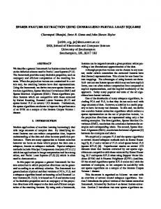
1 Introduuction 1.1: T second issue is the corruptive distortionn of the shaapes due to optical effeects like The i illumination n, perspectivve, aberratio on, chromaatism, high numerical n a aperture, etcc. While i general the in t three-diimensional shapes are expected to t be linearrly projected in the i image, such h optical effects e introoduce non--linearity innto the proojection. Thhus, for e example, a sphere mayy be projected as an elllipse or a line may distort to a hyyperbole. T Though theese distortioons are eassy to predict and som me mathem matical modeels may c completely explain theem, several other form ms of distorttions (like aberrations, a , motion b blurs, etc) are a quite com mplicated and a difficultt to invert or o interpret. Some exam mples of d distortions d to optical effects (ttaken from internet) due i aree presented in Figure 1.1-2. T third isssue is that of the senssor noise orr numerical noise. Duee to the pressence of The n noise in im mages, the edges becom me quibbledd or broken n into separrate contourrs. As a r result the loocal propertiies get seveerely affecteed and relatiing a brokeen edge curvve to the o original shaape becomees difficult.. Even worrse, it is possible p thaat the brokeen edge f fragment off one shape can be conffused as a part p of anothher shape. The T effects of noise a demonsttrated in Figgure 1.1-3. are

c by b noise (a) breakinng or shape corruption

(c) edges of o two shapees confused as one

(b) Quibbly efffect of noisse

Figure 1.1-3: Effect of sensorr noise or numerical n noise. n

4

Chappter 1: Introoduction A Another issuue is that thhe shapes often o appearr incomplete or mergess with otherr shapes d to overrlap and occlusion of the objects in the imaages. The edges due e of thee shapes o often becom me broken small fragm ments and it becomess difficult to t relate thhe small b broken edgees to their orriginal shap pes. See Figgure 1.1-4 fo or an exampple.

Figure 1.11-4: Illustra ation of thee presence of o overlapp ping and occluded ellipses

T These techn nical challennges make it i very difficcult to deal with geomeetric primitiives and t research the h in these toopics has beeen consistent but the progress p hass been limited. As a c consequenc e of these challeng ges, very complicateed algorithhms with lots of h heuristically y chosen coontrol param meters are used in praactice. As a consequence, the a applications s are very sensitive s to the choice of control parameterss [32-37] reelated to g geometric p primitives. T research The h presentedd in this thesis is basedd on the phiilosophy t that a betteer treatmennt of geomeetric primittives would d have sign nificant im mpact on a advanced i image proccessing appplications. The basic principle behind thhe work p presented in n this thesiss is that for each kind of geometriic primitivee, at least thhe effect o digitizatiion can be modeled of m with sufficiennt accuracyy. In most cases, c explicit error b bounds for the error inntroduced due d to digitiization can be derivedd. The errorr bounds In other f the digittization probblem can bee used for im for mproving th he existing algorithms. a c cases, insteead of using purely numerical n frramework for f applyin ng least squuares or c computing the t inflexioon points (w which are sensitive s to digitizationn and otherr noise), u unconventio onal means based on geeometry in the t two-dim mensional diiscrete planne can be u used to obtaain better soolutions to thhe difficult problems. I the next few sectionns, each of the In t followinng topics iss discussed from the foollowing r research perrspectives: 1. Reprresenting shhapes of thee digital curvves using appproximatin ng polygonss, 5

1.2: Introduction 2. Estimating tangents in digital curves, 3. Primitive ellipse fitting using edge pixels, and 4. Ellipse detection for practical scenario using hybrid approaches. Each of the above topics is significantly different from each other. For each of these topics, the challenges related to it, the background literature review, and a gist of the work presented in this thesis is presented.

1.2 Polygonal approximation of digital curves In several image processing applications [38-45], it is desired to express the boundaries of shapes (edges) using approximate polygons made of a few representative pixels (called the dominant points) from the boundary itself. Through polygonal approximation (PA), it is sought to represent a digital curve using fewer points such that: i.

The representation is insensitive to the digitization noise of the digital curve.

ii.

The properties of the curvature of the digital curve are retained, so that geometrical properties like inflexion points or concavities can be subsequently assessed.

iii.

The time efficiency of higher level processing can be improved since the digital curve is represented by fewer points.

Figure 1.2-1: Example of polygonal approximation of a digital shape.

An example is presented in Figure 1.2-1. In Figure 1.2-1, a digital shape of a maple leaf is illustrated. The boundary of the shape is made of 244 pixels. A PA of this shape 6

Chapter 1: Introduction is shown in Figure 1.2-1. The maple leaf is represented using only 27 dominant points in this approximation and the concavities associated with the maple leaf are preserved (labeled A-F). Despite being a very old problem of interest, this problem attracts significant attention even today in the research community. Some of the recent PA methods are proposed by Masood [36, 46], Carmona-Poyato [35], Ngyuen [37], Wu [47], Kolesnikov [40, 48], Bhowmick [49] and Marji [50] while a few older ones are found in [12, 13, 5160]. These algorithms can be generally classified based upon the approach taken by them. For example, some used dynamic programming [40, 48, 52], while others used splitting [12, 13, 53], merging [54], digitally straight segments [37, 49], suppression of break points [35, 36, 46, 50], curvature and convexity [47, 51, 55, 58]. Among the older methods, The method of Teh and Chin [51] relies primarily on the accurate determination of the support region based on chord length and the perpendicular distance of the pixels from the chords to determine the dominant points. Ansari [58] proposed a method in which a support region is assigned to each boundary point based on its local properties. A combination of Gaussian filtering and a significance measure is used on each pixel for identifying the dominant points. Cronin’s [59] method finds the support region for every pixel based on a non-uniform significance measure criterion calculated by locally determining the support region for each point. Ray and Ray [61] proposed a k-cosine-transform based method to determine the support region. Sarkar [62] proposed a chain code manipulation based method for determining the dominant points where the chain code is sufficient and the exact coordinates of the pixels are not necessary. Regarding the recent methods like Masood [46], Carmona-Poyato [35], and Nguyen [37], these methods have already shown considerable improvements over earlier dominant point detection or PA methods. However, all of these methods except Carmona-Poyato [35] use local properties of fit like the maximum distance (deviation) of the pixels on the digital curve from the fitted polygon. On the other hand CarmonaPoyato [35] uses a ratio ‘r’ which incorporates the quality of the global fit instead of the local fit. The reasons for the continued relevance of this problem in the current era are highlighted here: 7

1.3: Introduction 1. The performance metrics for evaluating the performance of a PA method, and 2. The control parameter and optimization goal used in the PA method. The technical details about these reasons are discussed in section 2.1. This thesis addresses both issues. Specifically, the work in this thesis has the following contributions to the PA problem: i.

Two simple metrics that relate to the global and local properties of fit of the polygon are proposed,

ii.

It is shown using these metrics that the global and local properties of fit are always conflicting in the least squares fitting scenario and that most existing PA methods optimize either the local or the global properties of fit,

iii.

A PA method based on simultaneous optimization of both the local and global properties of fit is proposed,

iv.

An upper bound of the error in line fitting due to digitization is derived,

v.

This upper bound is used to design a non-parametric framework which can be used to make most PA algorithms independent of control parameters and related heuristics,

vi.

The applicability of the framework is shown for a very popular PA method and two recently proposed PA methods, and

vii.

Experiments of various types are conducted to show the various practical aspects of PA problems and the performance of the proposed methods.

1.3 Tangent estimation for digital curves Tangent estimation (TE) is important in many applications like shape and perimeter estimations, concavity analysis, segmentation, etc. Despite the significant influence of the error in TE, most researchers tend to use heuristics and algorithms tailored specifically to the application. Also, they typically use complex optimization or curve fitting based algorithms that are computationally intensive, parameter controlled, sensitive to the digitization error, noise, and distortion. The problem of tangent estimation for digital curves had long been considered old and saturated [19-24]. However, a few researchers have begun to address the problem of tangent estimation for digital curves, with the specific aim of proposing criteria for evaluating the

8

Chapter 1: Introduction performance of tangent estimators and the development of better tangent estimators for practical applications [20, 21]. The problem of tangent estimation (TE) for digitized curves faces the following conceptual challenges: 1. The tangent is typically defined on a point, though it is a property of the continuous curve to which the point belongs. Thus, it has the local as well as the global properties of the curve. Due to digitization, both these properties are affected and the nature or extent of the effect cannot be quantified or analyzed using simple mathematical tools. At best, some estimates of maximum error or localized precision may be developed. 2. Usually, while estimating the tangents, prior information about the nature of the curve is unavailable. Further, appropriate size of the local region around a point is also unknown. Hence, the choice of these parameters is mainly heuristically guided and non-robust. One of the methods to find the tangent is to use continuous function (typically second order) to approximate the curvature of the digital curve in a local region around the point of interest [27, 63, 64]. The derivative of the continuous function is then used to determine the tangent. Such approach is restrictive in the choice of the nature of continuous function and the definition, shape, and dimension of the local region, etc. Further, there are applications where tangents need to be computed to fit a shape (for example ellipse) on the digital curve [25, 28, 45, 65]. In such cases, it is difficult to rely on a method that first fits a shape in the local region to estimate the tangent, and then uses the tangent to fit a shape to the whole curve. In order to overcome the problem of choosing the continuous function, researchers sometimes use a Gaussian filter to smoothen the digital curve and obtain a smooth continuous curve. This Gaussian smoothened continuous curve is then used for estimating the tangents [44]. In essence, this is similar to applying a one-dimensional spatial Gaussian filter. A similar approach is taken in [66], where one-dimensional spatial median filtering is used. Another method is to consider a family of continuous curves of various types. The complete digital curve is approximated by one of the continuous curves in the family using a global optimization technique. The tangents are then computed on the curve chosen by optimization [67]. A different approach is to 9

1.3: Introduction approximate the digital curves using line segments. Two main variations in this approach are in vogue. The first variation is based on the theory of maximal segments [20]. At the point of interest, the maximal line segments passing through it are found and weighted convex combination of their slopes is used to find the orientation of the tangent. This method is parameter-free, has asymptotic convergence, and incorporates convexity property. Though the theory of maximal segments is well-developed and fool-proof, the assumption that their weighted combination (and the value of the weights) is indeed a true representation of the curvature is based on heuristics, rather than analytic foundation. Despite that, to our knowledge, this is the first parameterindependent tangent estimation method (though involving heuristic choice of a function) that provides good properties in tangent estimation. The second variation is to approximate the digital curve using small line segments such that the maximum deviation of any point on the digital curve with one of the fitted line segments is small; for example, below a threshold value of a few pixels [44, 68]. This procedure divides the curve into small sub-curves each corresponding to a fitted line segment. The slope of the tangent at the midpoint of each sub-curve is then considered to be the same as the slope of the corresponding line segment. The main restriction with this method is that the tangents are available only at some points of the digital curves, viz., the mid points of the digital sub-curves. In our opinion, such method is essentially similar to the concept of maximal segments [20], especially if the threshold of the maximum deviation is less than or equal to 1.414 pixel. This thesis proposes a very simple and computationally efficient tangent estimator. It is shown that despite the simplicity of the method, the method has a definite upper bounded error for conics. Thus, this method does not suffer from the tangent estimation singularity experienced by other methods [31, 69]. The method uses a simple control parameter and a rule of thumb for choosing the control parameter is also provided. It is notable that the rule of thumb also uses the upper bound of the error in tangent estimation and thus it is less empirical than most other tangent estimation methods. Extensive numerical experiments validate the superiority of the proposed tangent estimator over almost all the existent tangent estimators. Further, the applicability of the proposed tangent estimator for non-conic curves with convex and concave curvatures is also exhibited.

10

Chapter 1: Introduction

1.4 Primitive ellipse fitting Ellipses appear in many natural objects ranging from cells and nuclei to astronomical bodies. Further, ellipses also appears commonly in man-made objects from medicinal tablets to space ships. Thus, using simple mathematical framework to detect ellipses from edge data has inspired many researchers. Initially, approaches like least squares fitting and Hough transform (HT) were the main approaches used by researchers. These approaches generally use the mathematical model of ellipse and the edge pixels for detecting the ellipses. Hough transform was introduced for ellipse detection in [14] in the form of simplified Hough transform (SHT). Modifications of Hough transform, randomized Hough transform (RHT) [70, 71] and probabilistic Hough transform [72, 73] were proposed to improve the performance of HT for non-linear problems like ellipse detection. HT based ellipse detection methods are usually more robust than least squares based ellipse detection when the edge contours are not smooth because they use pixels for detecting the ellipses instead of the edge contours (connected edge pixels) [74] while most least squares formulations for detecting ellipses use edge contours. HT based ellipse detection methods have two main problems. The first problem is that HT is computation and memory intensive because it uses a five-dimensional parameter space. For solving the problem of five-dimensional parameter space, many methods were proposed that split the five-dimensional space into two or more subspaces with lesser dimensionality and deal with each of the subspaces in separate steps [28, 75-78]. The most popular approach in these methods was to find the centers of the ellipses using geometrical theorems and Hough transform in the first step and finding the remaining parameters of the ellipses in the second step. Second problem is that since the pixels used in HT need not belong to the same edge contour, number of samples required for detecting each ellipse is very high. Once an ellipse is detected, the pixels near the detected ellipses are not considered for the detection of the next ellipse. Due to this, HT based methods may be unable to detect all obvious ellipses (represented by edge contours) and the accuracy of such methods reduces with the increase in the number of ellipses. Some methods used edge contours (instead of edge pixels) and piece-wise linear approximation of edge contours to improve the performance of HT [76, 79]. 11

1.4: Introduction Least squares based method was used for ellipse detection in [80-85]. Least squares based methods usually cast the ellipse fitting problem into a constrained matrix equation in which the solution should minimize the residue in the mathematical model. The choices of constraints and solution approaches for constrained matrix equations have an impact on the performance and selectivity of the ellipse detection methods [80, 83]. One problem with the least squares method is over-fitting of the data. Many pixels are used for ellipse detection and the elliptic hypothesis that minimizes the residue in the chosen mathematical equation and satisfies the constraint is generated. Thus, the chances of fitting an ellipse on a non-elliptic curve are high [84]. Second, though the amount of residue is used as the quality of fit and termination criterion, it may not necessarily be related directly to the quality of the detected ellipse. The least squares methods currently in use are based on the fundamental work by Rosin [82, 83, 86-88] and Fitzgibbon [80]. They both employ the algebraic equation of general conics to define the minimization problem and additional numeric constraints are introduced in order to restrict the solutions to the elliptic curves. In other works [86-89], Rosin developed and tested several error metrics for quantifying the quality of fit. Fitzgibbon [80] solves the constrained minimization problem using generalized eigenvalue decomposition. It is shown in this thesis that the method of Fitzgibbon [80] is prone to the problem of numerical instability and a simple modification of the method can make it numerically more stable. All the methods discussed above employ algebraic equation of the ellipse and the algebraic distance of the points on the ellipse as the cost function. As opposed to these, Ahn’s method [90] uses the geometric distances of the data points from the ellipse as the central quantity for fitting the ellipse. Ahn’s method involves nested iterative non-linear optimization, which makes it computation intensive and prone to the problem of local minima. Beyond this problem, Ahn’s method in general has a superior performance due to the fact that it uses minimization of the geometric distance instead of the algebraic distance which results in more physically relevant solutions. In both HT and least squares methods, if the points chosen lie actually on the loci of interest, the error in retrieval is expected to be very low. In such case, a small bin size is able to provide good precision [91]. However, actual points on the loci are hardly available from images, since the digitization rounds the coordinates of the actual points to the nearest integers [92, 93]. Digitization effect may impose severe 12

Chapter 1: Introduction restrictions on methods based on analytical equations. For example, it is easily conceivable that such methods will result into large errors for small circles and ellipses because the round off error due to quantization is of the order of the ellipse itself in these cases. Another example is the error in highly eccentric ellipses. However, the error may be non-negligible in other cases as well and may depend upon the choice of points [94]. Despite the practical importance of the effect of quantization on the accuracy of such methods, this issue has received least attention [91-93]. If such issues and their impact on the accuracy of these methods are understood, better techniques may be designed, reliable constraints may be introduced, and better methods may be chosen for achieving an acceptable accuracy in practice. This thesis proposes an ellipse fitting method based on least squares which uses the concept of minimizing the geometric distance of the data points from the ellipse to be fitted. However, as compared to Ahn’s method [90], the proposed method uses a linear least squares model and shifts the non-linearity involved in the determination of the geometric parameters of ellipse into a non-linear, but unique and easily computable operator. Further, the method is unconstrained and non-iterative. The proposed method performs superior to the remaining methods for various experiments and gives less false positives as compared to other methods. As a consequence, it is more suitable than other methods for the problem of detecting ellipses in images.

1.5 Ellipse detection for practical scenario using hybrid approach Ellipse detection in real images has been an open research problem for a long time. However, the performance is still poor for most real images like images of the Caltech 256 dataset [1]. Most hybrid approaches use a combination of pre-processing of edges for curvature correction, some or the other grouping scheme (usually based on edge continuity), primitive ellipse fitting algorithms (like discussed in section 1.4), elliptic hypotheses selection schemes, etc. Thus they are usually grouped under the umbrella term ‘hybrid ellipse detection methods’. While there are some sophisticated algorithms for detecting ellipses from images, most of these algorithms cannot be used in real time applications. Further, there is generally a least squares method at the core of these algorithms [80, 82, 83, 86, 87] and the other pre-processing and post-processing steps are used to increase the selectivity of the 13

1.5: Introduction algorithms to only elliptic shapes and reduce the false positives [25, 34, 68, 95, 96]. For instance, least squares methods typically need a fraction of a second, while extra processing steps used for improving selectivity may require a few seconds [34] to a several few minutes per image [33]. Furthermore, the selectivity of the ellipses can be poor and ellipses may be fitted in non-elliptic curves as well. For real time applications such as pupil tracking, where time is a critical parameter, a large number of processing steps are deemed undesirable and generally least squares method has to be used alone. Even for non-real time applications, it is desirable to have a least squares method that is inherently selective and good at reducing the false positives for non-elliptic curves, so that the burden on extra processing can be reduced. Researchers commonly use edge following methods for this problem, in which the connectivity of the edge pixels in the form of edge contours and the continuity of edge contours were used in addition to the mathematical model of ellipse [33, 34, 68, 81, 92, 97-99]. These methods work well for simple real images typically containing one or two ellipses in the foreground but fail to perform well in more complicated scenario such as presented in Figure 1.5-1.

(a) an example of real image

(b) its edge map (after histogram equalization and Canny edge detection)

Figure 1.5-1: An example of a real image and the problems in detection of ellipses in real images Some of the most notable articles are briefly discussed here. Mai [34] proposed a modified RANSAC (RANdom SAmple Consensus) [100] based ellipse detection method, which first extracts the fitted line segments from the edge data of the image. It follows an edge in terms of its continuity to group the edge with other edges. Finally, RANSAC based ellipse fitting is performed on these grouped arc segments. This method shows good performance in terms of accuracy and computational efficiency over many existing methods. However, the performance of this method is highly dependent upon the choice of the two thresholds – proximity distance and angular 14

Chapter 1: Introduction curvature. Split and merge detector proposed by Chia [101] in essence is the same. The performance of both these methods deteriorates in the presence of occluded ellipses. Hahn [102] proposed an ellipse detection method based on grouping points on elliptic contour. Whether some curved segments belong to the same ellipse or not, are tested by comparing the parameters of candidate ellipses that are made by the curve segments. This method can reduce the total execution time because it estimates the ellipse parameters in the curve segment level not in the individual edge pixel level. However, the performance of this method deteriorates for complex real images. Kawaguchi [103, 104] groups adjacent edge pixels with similar gradient orientations into the regions called as line-support regions, which are subsequently used for ellipse detection Ji [105] proposed a grouping scheme to pair the arc segments belonging to the same ellipse as an improvement over [81]. While [81] groups the edges based on a scale invariant statistical geometric criterion which can be verified either in parametric space or in residual error space, Ji [105] takes proximity and direction of arc segments (clockwise and counter clockwise) into account. Kim [68] proposed a grouping scheme based on three curvature and proximity based conditions as follows: an arc should be a neighbor in eight group classification [68], the arcs follow a convexity relationship as proposed in [78], and the inner angle between two edge pixel on an ellipse should not exceed 90 degree [68]. If the arcs satisfy these three constraints they represent circular arcs. In order to determine ellipses from the list of circular arc (obtained by merging three circular arc segments), it first finds the center of ellipse by center finding method [28]. Two arcs belong to one ellipse if they satisfy the parameters obtained by least squares method and the three constraints. These arcs are then merged and remaining elliptical parameters are extracted. One of the problems faced by any ellipse detection algorithm is that in attempts to detect all the ellipses actually present in real images in the absence of prior knowledge of the number of ellipses, they have to compromise on the accuracy of the algorithm. Any ellipse detection method, including the proposed method, suffers from the 15

1.5: Introduction problem of reliability and precision uncertainty. Due to this, the ellipse detection methods have to compromise on either the reliability or the precision. The popular choice is to compromise on the precision, as the quantization already limits the precision and due to the absence of a priori information on the elliptic objects present in the image, it is often important to be reliable in detecting the elliptic shapes. Due to this, often, the ellipse detection algorithms generate numerous elliptic hypotheses, not all of which correspond to actually present elliptic objects. Sometimes, many elliptic hypotheses are generated for a single elliptic object, and at other times, the hypotheses do not correspond to any actually present elliptic object in the image. Thus, it becomes important to evaluate the possibility of an elliptic hypothesis actually corresponding to an elliptic object. In other words, a method is needed to identify the elliptic hypotheses which are more likely to correspond to an object in image. Researchers use the ‘saliency’ or ‘distinctiveness’ scores for quantifying the reliability of a hypothesis [74, 97, 98, 106-110] and select the more salient elliptic hypotheses. Wang [109] presents some important work in this regard. But the measures suggested are neither simple nor computationally efficient. Further, the applicability of this method is restricted to Hough transform related ellipse detection methods and edge following methods. Basca [107] proposed a similarity measure that compares two elliptic hypotheses using the Euclidean distance between them in the Hough parametric space. Due to the absence of normalization, this method is sensitive to scale changes. Qiao [98] proposed ellipse detection method based on saliency of an arc. This method explores the relationship between spatial connectivity and the incremental point angle of elliptic inliers. This relationship can be used to detect elliptic arc end points. The angle subtended by the elliptic arc can then be used as ellipse validation criteria. This method depends on too many thresholds which are application dependent. This limits its use for wide range of application. The performance of this method depends on the proper choice of these threshold parameters. Another popular measure is the pixel count feature in [106]. Elmowafy [111] verified the elliptic hypotheses by checking the ratio of count of pixel on elliptic curve and approximated circumference of the ellipse. There are two major concerns regarding such scheme [97]. First, the pixels are an approximate (quantized) representation of the elliptic hypothesis. Due to this, in case of a complete elliptic edge, the number of pixels is more than the actual perimeter of the ellipse. Even if there is an incomplete 16

Chapter 1: Introduction edge, the edge represents a fraction of perimeter of the ellipse using more pixels than the actual length of the fraction. Second, the determination of perimeter of an ellipse is a classical problem in mathematics for which no closed form analytic solutions are available. The perimeter used is typically one among the various numerical approximations provided by scientists [112]. It is notable that all these approximations are subject to some assumptions that may not be generally valid for all the elliptic hypotheses generated. Also noteworthy are some of the steps related to edge data pre-processing, which is instrumental in enabling the detection of ellipses in real images. These include forming edge contours, removing junctions and branches [113], detecting inflexion points [114-118], obtaining edges of smooth curvature [33], etc. Among these, detection of the inflexion points is the most difficult problem. The reason is that inflexion points (or saddle points) are essentially defined by mathematical derivative in continuous space domain only. Continuous shape space (CSS) [115] based techniques like [117, 118] are noteworthy. These typically involve the convolution of the digital curve with a Gaussian kernel in order to transfer the curve into the CSS space and then use the persistence properties of the inflexion points in the convoluted CSS space to detect the inflexion points. Though the concept is interesting and apparently quite effective, it is complicated and involves significant amount of computation. Relatively simpler approach is taken in [116] but it depends strongly on three control parameters. Further, it is not specific to the inflexion points only and detects points with large curvature changes also since its aim is to detect the corner points and not specifically inflexion points. On the other hand, though Bai [114] is simple, it does not deal with all the possible situatiosn of inflexion points and its performance is control-parameter dependent. The hybrid ellipse detection method proposed in this thesis deals with almost all the issues raised above using simple approaches for each issue. Only a few control parameters are used in the proposed algorithm and the algorithmic design makes it less sensitive to the choice of control parameters. Specific contributions of the proposed method are listed below: i.

Simple inflexion point detection method based on curvature changes is proposed. The inflexion point detection method deals with more cases than 17

1.6: Introduction those dealt with Bai [114], is simpler than the inflexion point detection using curvature shape space [115, 118], and is parameter independent unlike [114, 116]. ii.

Grouping scheme which is not based on edge following method but still based on the curvature of the edges. Two simple schemes are used. The first is based on the search region for identifying the candidate edges for grouping. Second is based on the concept of associated convexity. For both of the scheme, simple and easily computable steps are needed.

iii.

Proposition of a non-linear trust score which gives more selectivity as compared to histogram score to Yuen’s method [28] for detecting centers of ellipses.

iv.

A simple similarity measure based on Jaccard index to determine similar ellipses.

v.

Three easily computable saliency criteria for dealing with various aspects of the quality of elliptic hypotheses.

vi.

A non-heuristic parameter-independent scheme for selecting ellipses that performs well for images of various kinds.

1.6 Practical applications In order to show the impact of the geometric primitives on practical image processing applications, three practical image processing problems are presented. The three applications are ellipse detection in real images, detection of cell organelles in extremely low contrast microscopy images, and object detection using polygonal and elliptic features only. For each of the applications, the core of the proposed algorithms is the geometric features. For detection of ellipses in real images, the hybrid ellipse detection method proposed in Chapter 5 is directly applied on images in the Caltech dataset [1]. It is notable that the method in Chapter 5 uses the PA methods and TE method proposed in Chapter 2 and Chapter 3. It also uses the improvement of Fitzgibbon’s method proposed in Chapter 4. For the application of detection of cell organelles, a scheme of pre-processing to improve the contrast and enhance the regions of interest is proposed. The least squares 18

Chapter 1: Introduction ellipse fitting proposed in Chapter 4 is then used for fast and accurate detection of the elliptic cell organelles. The method is easily parallelizable and it is possible to reduce the processing time to values close to the fluorescence microscopy acquisition time. Thus, it can be easily integrated in the microscopes. For the application of object detection in images, instead of conventionally used edge features, patch features, texture features, etc., the geometric features, i.e., PA of the edge contours and ellipses are used as the only features. In addition, a hierarchical template is used for object representation. The result of object detection for categories which have consistent geometric features is reasonably good. Indeed the performance can be enhanced by using other features like patch and texture features and this shall comprise the future work for this application.

1.7 Research not covered in the thesis While working on the doctoral topic, several related research topics were also explored. The research work related to these topics is briefly presented here. For instance, in the preliminary stage of the doctoral work, works on image composition analysis [119], a simpler ellipse detection scheme (as compared to the one presented in Chapter 5) [96], and a simple clustering scheme for ellipses were studied [120]. For the problem of object detection, contextual object detection for conscious machines [121] was studied. In addition to these works (directly related to the doctoral thesis), works related to cloud computing [122], embedded systems [123, 124], machine consciousness [121, 125-127], machine learning [128, 129], education data analysis [130], etc. were also done.

1.8 Outline and highlights of the thesis The thesis comprises of seven chapters. Chapter 1 and Chapter 7 present the introduction of the thesis and the conclusions respectively. Chapter 7 also presents some of the potential future directions. For the remaining chapters, the detailed outline is presented below. Chapter 2: Chapter 2 discusses the problem of polygonal approximation (PA). The contents of Chapter 2 have been reported in [93, 131-136]. After introducing the problem in 19

1.8: Introduction section 2.1, the global and local properties of polygonal fitting upon edge curves are discussed in section 2.2. Specifically precision metric for local quality of fit and reliability metric for global quality of fit are proposed in section 2.2.1. For least square fitting, it is shown in section 2.2.2 that the precision and reliability are always at conflict. This thus corroborates with the fact discussed in section 2.1.1 that the available metrics are not singly sufficient for PA. In this context, section 2.2.3 discussed whether the conventionally used performance metrics represent the global or local qualities of fit. Section 2.2.4 generalizes the precision and reliability metrics so that they can be applied to an edge curve, or an image with several edge curves, or a dataset with several images. Section 2.3 proposes a PA method that uses simultaneous optimization of both the precision and reliability metrics for an edge curve. The algorithm, called precision and reliability optimization (PRO), is proposed in section 2.3.1. Numerical experiments are presented in section 2.3.2. It is shown that the control parameter can be easily tweaked to obtain the desired performance of PRO. Section 2.4 presents a very important contribution of this chapter. It presents the analytical derivation of the error due to digitization of a continuous line segment in sections 2.4.1 and 2.4.2. Section 2.4.2 also proposes the non-parametric framework for PA. The error bound can be analytically derived and depends upon both the size and the orientation of the continuous line segment. This error bound is compared against other simpler error bounds proposed earlier by other researchers in section 2.4.3. Based on section 2.4.2, section 2.5 adapts three existing methods into the nonparametric framework and makes them parameter-independent. Section 2.5.1 makes the popular PA method proposed by Ramer-Douglas-Peucker [12, 13] parameter independent [132, 135]. Sections 2.5.2 and 2.5.3 make the recently proposed methods of Masood [46] and Carmona [35] parameter-independent [132, 133]. All the three methods are quite different from each other and yet the non-parametric framework can be used for them. The numerical results show that the non-parametric versions of these methods perform either better than or similar to the original versions of these methods. Even though other PA methods have not been adapted in the non-parametric framework, at least their optimization goals and update schemes are analyzed in the context of precision, reliability, and the analytical error bound in section 2.6. Various 20

Chapter 1: Introduction interesting and practical aspects of PA methods are analyzed in section 2.7. In this section, the performance of the methods proposed in sections 2.3 and 2.5 are compared for scalability, noisy curves, non-digitized curves, and performance over large datasets of practical use. Some recommendations regarding the choice of PA methods in practical applications are provided in section 2.7.5. The chapter is concluded in section 2.8. Chapter 3: Chapter 3 considers the problem of tangent estimation (TE) for digital curves. The content of this chapter have been reported in [31, 69]. After providing the background of the problem in section 3.1, an example is shown in section 3.2 which highlights the importance of reducing the error in TE. The tangent estimation method proposed in this thesis appears in section 3.3 in which the concept, algorithm, and the computation complexity of the method are discussed. There is only one control parameter which can be chosen using a thumb rule presented in section 3.4.3. Section 3.4 is an important highlight of this chapter. The error in tangent estimation has been analytically derived for the continuous conics in section 3.4.1. The error in tangent estimation due to digitization of the continuous conics and the total error bound (sum of error bounds for continuous and digital curves) are presented in section 3.4.2. Section 3.4.3 discusses the choice of control parameter which is based upon the total error bound and the smallest circle of interest. In the same section, the multigrid performance of the presented method is also discussed. Section 3.5 presents several numerical simulations to illustrate the error bound for conics of various types. Section 3.6 also presents a highlight of this chapter. In this section, the performance of the proposed method is compared against almost all the existing tangent estimation methods and it is seen that the proposed method perform superior to all of them. Besides considering circular and elliptic geometries, some non-conic curves are also considered and it is seen that the proposed method performs quite well for all the geometries. The chapter is concluded in section 3.7. Chapter 4: Chapter 4 considers the problem of least squares fitting of ellipses. The contents of this chapter have been reported in [25, 137-139]. After introducing the problem of least 21

1.8: Introduction squares fitting of ellipses and the state of the art in section 4.1, the conventionally used algebraic fitting of ellipses is presented in section 4.2. Specifically, the popular method of Fitzgibbon [80] is considered in this section and the problem of numerical instability of this method is discussed. Based on the discussion, a simple solution for dealing with this numerical instability is proposed in section 4.2.2. The concept of geometric distance minimization is discussed in section 4.3. The geometric equation of a general ellipse, its simplified form, and the distance of a data point from the ellipse to be fit is presented here. These expressions are useful for the theory presented in section 4.4. Section 4.4 is the highlight of this chapter. For the subsequent use of linear unconstrained least squares method, a modification of the minimization function (the geometric distance) is proposed in section 4.4.1. The mathematical model of the method is proposed in section 4.4.2. The model of fitting involves using two operators and an intermediate unknown parameters space such that one operator is linear and the other operator is non-linear. By the properties of the linear operator and the definition of the intermediate parameter space, linear unconstrained least squares minimization of the residue can be used for determining the intermediate variables. The non-linear operator, its injective mapping, and inversion are presented in section 4.4.3. The numerical stabilization of the linear operator is discussed in section 4.4.4. Finally the computational complexity of the proposed method is presented in section 4.4.5. Several numerical simulations and comparison with other least squares methods are presented in section 4.5. The proposed method performs better than the other least squares method for variety of cases like digital incomplete curves, noisy clusters of data points, as well as images with several incomplete ellipses. The proposed method is also tested for non-elliptic conics and non-conics as well and it is seen that the proposed method has lower false positives as compared to other least squares based methods. The chapter is concluded in section 4.6. Chapter 5: Chapter 5 proposes a hybrid advanced ellipse detection method. The contents of this chapter have been reported in [45, 95, 96, 139]. The background introduction to the proposed method is presented in sections 5.1 and 5.2 respectively. Preprocessing of 22

Chapter 1: Introduction edge curves is proposed in section 5.3. One of the important contributions of this chapter is the method for finding inflexion points in digital curves, which is described in section 5.3.2. Grouping and elliptic hypotheses generation is proposed in section 5.4. The concepts of search region and associated convexities proposed in sections 5.4.1 and 5.4.2 are some highlights of this section. A non-linear relationship score for grouping and ranking the edges in a group is proposed in section 5.4.4. This relationship score is more selective than the usual histogram score and thus provides more robust grouping and ranking of the edges. Section 5.5 is an important contribution of this chapter. Section 5.5.1 proposes a simple and elegant method of detecting similar elliptic hypotheses using Jaccard index. Section 5.5.2 presents three saliency score, which can be easily computed and represent different aspects of the quality of the elliptic hypotheses. Section 5.5.3 presents several ways of combining the saliency scores and studies the issues with each combination. Section 5.5.4 proposes a hypotheses selection scheme which does not require user specified thresholds or filtering parameters. The scheme is nonheuristic and determines the suitable values of threshold from the image itself. The scheme works well for most images. Several numerical evaluations and comparison with other methods are presented in section 5.6. It is seen that the proposed method performs much better than several other hybrid methods. The chapter is concluded in section 5.7. Chapter 6: Chapter 6 presents three practical applications in which the geometric primitives discussed in Chapter 2 to Chapter 5 are used. The first application – detection of elliptic shapes in real images of Caltech 256 dataset [1] – is presented in section 6.1. The contents of this section are presented in [45]. It is noted that the method presented in Chapter 5 performs better than most other hybrid methods and provides reasonable performance for use in practical applications. Section 6.2 presents the biomedical application of detecting cell organelles from microscopy images. Its contents has been reported in [140]. The highlight of the method proposed for this problem in section 6.2.1 is the preprocessing. The discussion 23

1.8: Introduction in section 6.2.1.1 shows how the gray scale histogram for all the images in the dataset can be used for improving the contrast of the images (which have extremely poor contrast). The method shows very good performance. Further, it is shown that the time taken by the method for each image can be pushed to below 1 second using parallel computing and more efficient openCV and C++ implementations. Section 6.3 presents the application of object detection in images. Its contents has been reported in [141]. The object detection method presented in this section uses only approximating polygons and detected ellipses as the features of the object. The hierarchical object representation template with generative and discriminative capabilities presented in section 6.3.1 is a highlight of this method. The performance of the object detection method is shown for 16 object categories spread over two datasets. Chapter 7 and Appendix: Chapter 7 presents the conclusion and potential future directions of this thesis. There are six appendices labeled Appendix A - F. Appendix A provides an important proof for a theorem used in Chapter 2. Appendices B - D provide important derivations of the expressions in Chapter 3. Appendices E and F concern Chapter 6. Appendix E provides the details of the tool used for generating the ground truth for section 6.1. Appendix F provides a brief summary on the various aspects of object detection methods.

24

Chapter C 2: Polygonal P a approximati on of digitaal curves

Chaptter 2 : Polygonaal approximatioon of diggital currves

2 Backgground 2.1 I this chap In pter, the probblem of rep presenting a digital currve as a polyygon is connsidered. T problem The m of polygoonal approxiimation (PA A) of digitall curves is often o cast ass either a m min-# probblem or a min-  prroblem [1442]. Both the t problem ms are esssentially m minimizatio on problemss. However,, the formerr’s aim is to o find the minimum m nuumber of p points such that the vaalue of a paarticular errror functionn is below a certain thhreshold, w while the laatter’s aim is i to find a fixed numbber of dominant points such that the t error f function hass minimum value. Recently, severral methodss have been proposed to obtain t PA of digital the d curvves in the framework f of min-# problem. p Thhis is becauuse it is d difficult to determine d t fixed nuumber of pooints in minn-  problem the m suitably for fo many s shapes, while if the errror function in min-# iss related to the quality of fit, it is easier e to u heuristiccs to determ use mine a generrally accepttable threshoold for the error e functioon. A rigorous literature l reeview of thee problem reeveals that the t problem m is quite old. Some o the initiall works in thhis topic aree [12, 52, 55, 61, 62, 142-149]. Despite severral years of o research and appareent simplicitty of the prroblem, it remains of r releevant in thee current e as well [35-37, 40, 42, 46-50, 57, 60, 64,, 150-159]. The reason era ns for the coontinued r relevance off this probleem in the cuurrent era arre highlighteed here: 1. Thee performannce metrics for f evaluating the perfoormance of a PA methood. 2. Thee control parrameter andd optimization goal useed in the PA A method. 2 2.1.1 Perforrmance meetrics F First, even though maany algorith hms were ddeveloped for PA of digital currves, the m metrics used to compaare and ben nchmark vaarious algoorithms werre not effecctive, as s shown in [1149, 159]. Researchers tried usinng absolute performan nce metrics such as c compression n ratio, inteegral square error, figurre of merit, zero norm,, infinity noorm, etc. S Studies provved that such metrics fail to reprresent the quality q of fit in one maanner or a another [151, 159]. Thhe reason foor this was not understtood fully. This T chapteer shows t that there iss a perenniaal conflict in n the qualityy of fit in thhe local scaale (precisioon at the 25

2 Polygonnal approxim 2.1: mation of digital d curvees l level of a feew pixels) and a global scale s (reliabbility at thee level of coomplete currve) [93, 1 134]. This duality d of precision p annd reliability of a fit haunts h mostt fitting algorithms. T This aspect is highlighhted in sectiion 2.2.2. Due D to this reason, mo ost absolute metrics f in properly quantifying the quality fail q of fiit. The exissting absoluute measurees in the c context of loocal and gloobal quality y of fits are presented p inn section 2.2 2.3. It is shoown that t absolutee metrics eitther concenntrate on thee local or th the he global naatures of fit. Several P methods are studieed in the context PA c of the t local an nd global natures n of fitting f in s section 2.6. R Researchers s tried relatiive measurees like fidelity, efficienncy, and merit m to quanntify the q quality of fit [149, 159]. 1 In relative meassures, a soo-called optimal algorrithm is c considered as the refeerence for comparing c the perform mance of thhe algorithm m being t tested. The method prooposed by Perez P and Vidal [52] baased on dynnamic progrramming i generally is y used by the t researchhers as the reference algorithm. This is beecause it

m  # such that the fitting erroor is minim minn   and min t targets mized for a certain n number of points p ( min   ) or the number of points for fitting f is minnimized forr a given v value of fittting error ( min # ). It I is logicall that there is no way of determiining an o optimal valu ue for the fixed numbber of pointts ( min   ) or the fix xed value of o fitting

 # ), becausse such a vaalue dependds upon the nature of thhe digital curve e error ( min c for w which PA iss sought. One PA methhod that usees the precision and relliability meetrics for P is propoosed in sectiion 2.2.4. PA 2 2.1.2 Contrrol parametter and opttimization goal g A mentionned above, heuristics are involveed in choossing the threshold (foor min-# As p problem) orr the fixed number of points (in minm  probblem). The control parrameters u used in mosst PA methoods are ofteen related too the maxim mum deviatiion of the pixels p on t digital curve the c segm ment betweeen adjacent dominant points from m the line segment are relatedd to the c connecting the dominnant points. When thee control parameters p m maximum deviation, the allowaable or tolerable maaximum deeviation is chosen h heuristically y as a threshold value. Although the threshoold is generaally chosenn to be a c constant, a suitable s vallue of the th hreshold varries from on ne digital cuurve to another and e even within n the digitall curve. Hoowever, no specific rules are available for choosing c e either the coonstant threeshold valuee or an adapptive threshhold value depending d u upon the d digital curvee. 26

Chapter C 2: Polygonal P a approximati on of digitaal curves T This thesis proposes a non-paraametric fram mework forr the autom matic and adaptive a d determinatio on of the threshold t fo or the min--# problem.. A theorettical boundd for the m maximum deviation d off a set of piixels by diggitizing a liine segmennt is first deerived in s section 2.2.44. This expplicit and annalytically defined d bou und is relateed to the lenngth and t slope of the line segment. the s Thhis bound is compareed to other theoretical bounds r related to thhe digitizatioon of contin nuous line segments annd it is show wn that this bound b is m more versatile than the other boun nds. T maxim The mum possiblle deviation n due to digitization can c be com mputed for any a line possible s segment using the prooposed erroor bound. Thus, T the computed c m maximum d deviation caan be easilyy used as a threshold t foor each individual edgee of the polyygon. In t sense, it this i serves as a natural benchmark ffor any dom minant pointt detection method. T applicaation of thee proposed non-param The metric framework in the t dominannt point d detection m methods is demonstrate d ed in sectioon 2.4.3. Three T popular PA methhods by R Ramer, Douuglas, and Peucker P [122, 13] (referred to as RDP), Masoood [46] (refferred to a Masood)), and Carmona-Poyaato [35] (reeferred to as Carmon as na for brevvity) are a adapted in the propossed non-parrametric fraamework. The T modifi fied non-parrametric v versions off the methods are caalled RDP--mod, Masood-mod, and a Carmoona-mod r respectively y. T adaptedd versions of the meth The hods are coontrol param meter indeppendent andd do not r require userr specified inputs i (thuss making thhese algorithhms free fro om heuristics). The m modified m methods shoow balanceed performaance over their t origin nal version despite b being controol parameteer independeent. The bouund based non-parame n etric framew work can b easily inttegrated in other PA or Dominantt point detection metho be ods as well and can b used too make theem non-heu be uristic (or less heuristic) and self-adaptiv s ve. It is the basic construct h highlighted that in the proposed framework, f c annd the naturre of the remain uncchanged, while a algorithms w only optimization o n or terminnation conddition is a altered in orrder to makee the metho od non-param metric. 2 2.1.3 Experriments forr PA methoods F investig For gating the pperformancce of the foour PA meethods propposed in thiis thesis ( (Precision Reliability R O Optimizatio on (PRO), RDP-mod, R M Masood-mo od, Carmonna-mod), q quantitative and qualitaative analyssis of the methods m for 18 standardd digital shaaped are u used to asssess PA methods. m In addition to t this, som me interestting and im mportant 27

2 Polygonnal approxim 2.1: mation of digital d curvees e experiments s that reflecct interestingg and usefuul propertiess are considdered in secttion 2.6. T The first experiment e studies thee performaance of PA A methods for digitall curves ng to scaledd versions of c correspondi o the samee shape. Thee second ex xperiment coonsiders t perform the mance of the PA methhods for nooisy digital curves. Thhe third expperiment i investigates A methods can be appplied for seemi-digitizeed or non-ddigitized if the PA c curves reprresented byy discrete points witth real valued coordiinates. In the last e experiment, the perform mance of thhe PA methhods over laarge datasetts of real im mages is c considered. In general,, the perform mance metrrics are defi fined for a single s digitaal curve. H However, fo the last experimentt, it is impoortant to finnd generalizzed versionns of the for p performance e metrics which w can reepresent thee performan nce of PA methods m for a set of i images, each h containingg several diigital curvess. 2 2.1.4 : Outliine and maajor contrib butions T global and The a local prroperties off polygonal fitting upon n edge curv ves are discuussed in s section 2.2. Such an annalysis of thhe global annd local propperties of fiit has been done d for t first tim the me in this ddoctoral. Preecision mettric for locaal quality of o fit and reeliability m metric for global g qualitty of fit are proposed in i section 2.2.1. For leaast square fitting, f it i shown in section 2.22.2 that the precision and is a reliabiliity are alwaays at confliict. This t thus corroboorates with the fact disscussed in section s 2.1.11 that the avvailable meetrics are n singly sufficient not s foor PA. Sectiion 2.2.3 diiscussed whhether the conventiona c ally used p performance e metrics represent r t the global or local qualities q of fit. Sectioon 2.2.4 g generalizes the precisioon and reliaability metriics so that they t can be applied to an edge c curve, or an n image withh several eddge curves, or o a dataset with severaal images. S Section 2.3 proposes a novel PA method thaat uses simuultaneous opptimizationn of both t precision the n and reliabbility metriccs for an eddge curve. The T algorithhm, called pprecision a and reliabiility optim mization (PRO), is proposed p i section 2.3.1. Nuumerical in e experiments s are presennted in sectiion 2.3.2. Itt is shown that the conntrol param meter can b easily tw be weaked to obbtain the dessired perforrmance of PRO. P S Section 2.4 presents a very imp portant conttribution off this chaptter. It presents the a analytical derivation d of the error due to digiitization off a continuo ous line seggment in s sections 2.4 4.1 and 2.4..2. Sectionn 2.4.2 also proposes the t non-parrametric fraamework f PA. Thee error bounnd can be analytically for a derived annd depends upon both the size a the orientation off the continnuous line segment. This and T error bound b is coompared 28

Chapter C 2: Polygonal P a approximati on of digitaal curves a against otheer simpler error boundds proposedd earlier byy other reseearchers inn section 2 2.4.3. S Section 2.5 adapts threee existing methods m intto a novel non-paramet n tric framew work and m makes them m parameterr-independent. The threee methodss are quite different d froom each o other and yet y the non--parametric frameworkk can be used for them m successfuully. The n numerical r results show w that the non-parameetric versioons of thesee methods perform e either betterr than or sim milar to the original verrsions of theese methodss. T optimizzation goals and updaate schemess of severall methods are The a analyzed in the c context of precision, p reeliability, an nd the analyytical error bound in section 2.6. Various i interesting a practical aspects of and o PA methhods are annalyzed in section 2.7. In this s section, the performancce of the meethods proposed in secttions 2.3 annd 2.5 are coompared f scalabiliity, noisy cuurves, non-d for digitized cuurves, and peerformance over large datasets o practicall use. Som of me recommeendations regarding r thhe choice of o PA metthods in p practical appplications are a providedd in section 2.7.5. The chapter c is concluded inn section 2 2.8.

2 Local and global qualitiees of fit 2.2 2 2.2.1 Precission and reliability meetrics T This sectionn presents the recently proposedd precision and reliabiility criteriaa which r represent th he local andd global natuure of fittinng. Supposee a digital curve c is reprresented u using a seequence off connecteed pixels S  Pi  xi , yi  , i  1 to M

and it is

a approximate ed using a liine ax  by  1 . F considering the loccal characteristics of fittting, it is useful For u to com mpute the algebraic a d distance of the t pixels Pi  xi , yi  from the line ax  by  1 . Thus, the precision metric m of f fitting can be b modeled using the noormalized rresidue giveen in eqn. (22-1):

 p  w where X   x1 

x2 

xM 

T

 y1

XA  J A

2

(2-1)

2

y2 

T T y M   , A   a b , and J is a 

c column mattrix containning M row ws, the everry element of o which iss 1. The supperscript 29

2 Polygonnal approxim 2.2: mation of digital d curvees

T denotes the transpose operationn and 

p

p  norm r represents the t m of vectorrs. Since

c tic of the local nature of o fitting  p considerrs the residuue for each pixel, it is characterist a alone. O the otheer hand for the global characterist On c ics of fit, reeliability off a fit referss to how w the fit is well i expected to satisfy att least two conditions: c The fit should be valid foor a sufficieently large region (or in this casee a long

i.

curvve). ii.

It sh hould not bee sensitive to o occasionaal spurious large l deviations in the edge. e

A combinattion of bothh these prop perties can be b sought by b defining a reliabilityy metric a shown inn eqn. (2-2). as

r 

XA  J

1

smax

(2-2)

smax is the maxximum Eucllidean distannce betweeen any two pair of pixeels [93]. w where H Here,



reprresents the magnitude or the absollute value.

2 2.2.2 Dualitty of precission and relliability I a line ax  by  1 hass to be fitted on the diggital curve S , then thee coefficientts of the If

a and b , can be determined l line, d b solving the by t matrix equation e [16 60] of eqn. (2-3) ( for t vector A : the

XA = J ,

(2-3)

T The above equation is i clearly an a over-determined equation. e Fuurther, duee to the d discretizatio on, the inteeger co-ordiinates (pixeels) closest to the requuired line may m not e exactly lie on the linee. Accordingg to the coonsistency criterion, c eqquation (2-33) has a u unique soluttion only when w the ran nk of X annd  X J  iss same [1611]. It is notaable that d to the discretizatio due d on in pixels,, xi and yi being inteegers, the coonsistency criterion c i satisfied only is o in fourr cases: a perfectly horrizontal linee, a perfectlly vertical line, l and t lines with slopes 1 . These caases are shoown in Figuure 2.2-1(a-d). For thesse cases, the t there are exaactly two inndependent rows in X and the sollution is uniique.

30

Chapter C 2: Polygonal P a approximati on of digitaal curves

Fiigure 2.2-1: Exampless of digital curves (lin nes) for the precisionreliability duality.

F all the other For o cases,, using leasst squares method, m the above equaation can bee solved f minimum for m residue as in eqn. (2--4) below [1160, 161]:



A = XT X



-1

XT J .

(2-4)



N Now, usingg the abovve solution in eqn. ((2-1) and assigning B  X X T X



C  X XT X



2

m can be b written as a in eqn. (2 2-5) below: X T , thee precision metric

31



1

XT ,

2.2: Polygonal approximation of digital curves

 BJ  J   BJ  J  T

 p  

AT A J

T

I  B J J T CJ



JT  B  I 

T



B  I J

J T CJ

 I  B  C







J T B T B  B  BT  I J J T CJ

M B C

where I is the identity matrix of size M ,

(2-5)

 A represents the sum of all the elements

of the matrix A and the properties of matrix B and vector J in eqn. (2-6) and (2-7) respectively are used:

B  BT  BT B

(2-6)

J T AJ   A

(2-7)

Further, it is proven in Appendix A that eqn. (2-8) below is valid:

B  M

(2-8)

Thus, it is evident from eqn. (2-5) that the precision metric  p can be reduced by choosing lesser number of pixels M . It should be noted that with the decrease in the number of pixels, X and consequently B and C change. This in effect amount to saying that fitting the line in a smaller local region is more precise than a large region. From eqn. (2-2), since a sequence of pixels is considered, smax can be high if and only if the number of pixels M is high. Thus, there is always a contradiction between precision and reliability. In order to increase the precision, smaller regions should be considered for fitting, whereas for increasing the reliability, larger regions need to be considered (largest region being the region spanned by the connected edge pixels under consideration). Indeed the contradiction does not occur in ideal lines as shown in Figure 2.2-1 (a-d). Further, the contradiction is not an issue if the lines are in general smooth, so that the precision within a large region is already very high, such that reliability and precision are already sufficiently high and there is no practical need to increase the precision or reliability. Some such examples are presented in Figure 2.2-1(e-g) and the lack of contradiction in such cases is seen in Figure 2.2-2 (e-g) and Table 2.2-1.

32

Chapter C 2: Polygonal P a approximati on of digitaal curves

Figure F 2.2-2: Fitted lin ne (red asterisks) on the t digital curves in u the leeast squaress approach h. Figgure 2.2-1 using

T Table 2.2-11: Precision n and reliab bility metriics for Figu ure 2.2-2. Digitall curve Precision metric  p Reliability metric  r Digitall curve Precision metric  p Reliabilityy metric  r Digitall curve Precision metric  p Reliabilityy metric  r Digitall curve Precision metric  p Reliabilityy metric  r

Figure 2.2-2(a)

Figuure 2.2-2(b)

Figure 2.2-2 2(c)

Figuree 2.2-2(d)

0.0000

0.000

0.000

0 0.000

0.0000

0.000

0.000

0 0.000

Figure 2.2-2(e)

Figuure 2.2-2(f)

Figure 2.2-22(g)

Figuree 2.2-2(h)

0.0244

0.035

0.013

0 0.071

0.0222

0.031

0.008

0 0.066

Figure 2.22-2(i)

Figuure 2.2-2(j)

Figure 2.2-22(k)

Figuree 2.2-2(l)

0.0477

0.015

0.072

0 0.121

0.0488

0.007

0.057

0 0.114

Figure 2.2--2(m)

Figuure 2.2-2(n)

Figure 2.2-22(o)

Figuree 2.2-2(p)

0.1500

0.111

0.121

0 0.233

0.1355

0.107

0.115

0 0.248

33

2 Polygonnal approxim 2.2: mation of digital d curvees E Examples of o more pracctical cases are shown in Figure 2.2-1(h)-(p) 2 . In such caases, the c contradictio on comes innto picture strongly s as seen s in Figuure 2.2-2(h--p) and Tabble 2.2-1 (values are shown s till 3 decimal pooints.). For practical reepresentatio on of the cuurves in t these cases, a balance has h to be achieved suchh that the fitt is sufficien ntly reliablee as well a precise. as 2 2.2.3 Existing perform mance metrric in the coontext of prrecision and reliabilityy I this secttion, the abbsolute perfformance metrics In m gen nerally used d for assesssing the q quality of fiit are discusssed in the context c of the t precisionn and reliab bility metriccs (eqns. ( (2-1) and (2 2-2) respecttively). The aim here iss to investiggate if the pperformance metric u under considderation in this sectionn represents local qualitty of fit or global g qualitty of fit. 2 2.2.3.1 Maxximum deviiation (MD,, max(di ) ) S Suppose thee minimum distance foor each pixeel on a digittal curve froom its apprroximate p polygon is computed. This distaance is callled the devviation of the t pixel fr from the p polygon. Thhe maximuum deviatioon (MD) off a digital curve from m its polyggon then c corresponds s to the pixel for whicch the deviaation is max ximum. Forr conveniennce, it is r referred to as MD or max(di ) . For F a generral line giveen by eqn. (2-3) fittedd upon a d digital curvee (or its porrtion), max((di ) is specified by eqnn. (2-9) beloow: max(ddi )  XA  J

S Since 



 

2



A

2

(2-9)

di ) is a [112]], max( d i )   p . Thus,, it can be concluded that max(d

f form of preccision (locaal fit) measuure. 2 2.2.3.2 Integ gral squaree error (ISE E) I Integral squ uare error (IISE) is the sum of squuares of dev viations of the t pixels from f the a approximate e polygon iss given by eqn. e (2-10) below: b

 

ISE=  p

2

(2-10)

T Thus, effecttively, ISE is i also a preecision (locaal fit) measuure. 2 2.2.3.3 Dim mensionalityy reduction (DR) ratio or compresssion ratio (CR) ( T compreession ratioo given in eqn. The e (2-11)) is the ratiio of numb ber of pixells in the d digital curvee ( N ) to thee number off vertices off the approx ximate polygon ( M ), 34

on of digitaal curves Chapter C 2: Polygonal P a approximati CR  N M

(2-11)

T Though thiss measure is not related to either precision or o reliabilityy, it is an im mportant p performance e metric in practice. A larger valuue of CR is beneficial for f the reduuction of d data and computationnal resourcees for furthher higher level proccessing. Insstead of c compression n ratio, its reciprocal dimensionaality reductiion ratio giiven in eqnn. (2-12) c be used as a minim can mization mettric (i.e. the lesser, the better). b

DR R  CR 1  M N

(2-12)

2 2.2.3.4 Figu ure of meritt (FOM) F Figure of merit m (FOM) is given by y eqn. (2-13): F FOM = CR ISE

(2-13)

T This is a maximization m n metric, i..e., larger value v of FO OM is prefe ferred over a lower v value. Howeever, it is w well known that t FOM iss biased tow wards ISE [3 35]. For exaample, if t break pooints of a diigital curvee [46] are coonsidered ass the dominnant points, the ISE the i zero and is d inconsequuent of the CR, FOM is infinity y. If a miniimization metric m is p preferred, s deficiiency as WE W 1 =1/FOM M [50] maay be used.. It suffers with the same F FOM. 2 2.2.3.5 Disccussion I is notablee that most important metrics It m use local qualiity of fit. Thhere are harrdly any m metrics that use the gloobal quality of fit. The logic that iss probably applied a is thhat if the f fitting is locally good for individdual curve segments, the quality of fit all over o the d digital curvee is also goood. Howevver, as show wn earlier inn section 2.2 2.2, there iss often a c contradictio on between the local annd global qualities q of fit, i.e., a very v preciseely fitted c curve may not n be a reliable fit. 2 2.2.4 Generralizing preecision and d reliabilityy metrics foor datasets T section This n extends thhe precision n and reliabbility metriccs presentedd in equatioons (2-1) a and (2-2) to t the casees of digitaal curves, images, annd datasets.. Suppose J line s segments arre fitted uppon a digitaal curve. A Also, supposse that an image conttains K d digital curvees and a dattaset containns L imagees.

35

2.2: Polygonal approximation of digital curves 2.2.4.1 Precision metric The net precision metric for the digital curve is defined as follows in eqn. (2-14) [134]:

 p  mean   pj ; j  1 to J  ,

(2-14)

j where  p is the precision metric of the j th line segment, defined using eqn. (2-1).

Since an algorithm is applied on one digital curve in one execution, hence taking the mean in eqn. (2-14) is reasonable. Further, since precision is a local property of fit, it can be defined only for the individual line segments and therefore the net precision accounts for the precision of every line segment. The precision metric of an image is defined as in eqn. (2-15):

 p  max   pk ; k  1 to K  ,

(2-15)

k where  p is the precision metric of the k th digital curve, defined using eqn. (2-14). It

should be noted that instead of taking the mean as in eqn. (2-14), max is used for computing the metric for an image in eqn. (2-15). This is because one curve may differ from another curve in an image due to various factors like the shapes, lighting, noise, etc. in the image. The precision metric of a dataset of images is defined as in eqn. (2-16):

 p  mean   pl ; l  1 to L  ,

(2-16)

l where  p is the precision metric of the l th digital curve, defined using eqn. (2-15).

Taking the mean as the metric for an image is reasonable. 2.2.4.2 Reliability metric The net reliability measure of the digital curve is defined as follows in eqn. (2-17) [134]: J

r   X jA j  J 1 j 1

J

j ,  smax

(2-17)

j 1

j correspond to X , A , and smax in eqn. (2-2) for the j th line where X j , A j , and smax

segment. The above definition in the context of a digital curve is consistent with the concept of reliability metric as a metric of global fit. Thus, the net reliability measure 36

Chapter 2: Polygonal approximation of digital curves does not consider the reliability measure of individual segment. Rather, the individual constituents of reliability measure (the numerator and denominator in eqn. (2-17)) are computed using all the segments. 2.2.4.3 Other performance metrics Following four performance metrics are also generalized for an image or a dataset. 1. Compression ratio (CR): Compression ratio for an image is computed as the average CR of all the digital curves in an image. Similarly, the compression ratio of a dataset is computed as the average CR of all the images in the dataset. 2. Maximum deviation (MD): MD for an image is computed as the average MD of all the digital curves in an image. Similarly, MD of a dataset is computed as the average MD of all the images in the dataset. 3. Integral square error (ISE): ISE for an image is computed as the average ISE of all the digital curves in an image. Similarly, ISE of a dataset is computed as the average ISE of all the images in the dataset. 4. Figure of merit (FOM): FOM for an image is computed as the average FOM of all the digital curves in an image. Similarly, FOM of a dataset is computed as the average FOM of all the images in the dataset.

2.3 Algorithm based upon precision and reliability optimization (PRO) In this section, a method designed to optimize both the precision and reliability is proposed. Since this method optimizes both the precision and reliability metrics, it is referred to as the precision and reliability based optimization (PRO) method. For the ease of further reference, a distance function is defined in eqn. (2-18): d  a , b, p  

x p  ya  yb   y p  xb  xa   yb xa  ya xb

 xb  xa 

2

  y a  yb 

2

.

(2-18)

This distance function denotes the distance of a point Pp  x p , y p  from the line passing through two points Pa ( xa , ya ) and Pb ( xb , yb ) . This distance function shall be used several times in this chapter and has been pre-defined for the ease and simplicity 37

2 Polygonnal approxim 2.3: mation of digital d curvees o referencee. This funcction appliess to points as of a well as pixels p and thhe argumennts a , b , a and t subscrippts of the pooints in conssideration. p are the 2 2.3.1 Precission and Reeliability baased Optim mization (PR RO) C Consider a digital curvve S  P1

t edge pixeel in the P2 ... PN  , where Pi is the i th

d digital curvee e . The linne passing through a pair p of pixels Pa ( xa , ya ) and Pb ( xb , yb ) is g given by eqn n. (2-19): x  ya  yb   y  xb  xa   yb xa  ya xb  0 .

(2-19)

T deviatiion d i of a pixel Pi ( xi , yi )  S from the line The l passing g through the pair

P1 , PN 

is then t given by b eqn. (2-2 20): d i  d 1, N , i  .

(2-20)

A Accordingly y, the pixel with maxim mum deviattion (MD) can c be found d. Let it be denoted a Pmax . Considering thhe pairs  P1 , Pmax  andd Pmax , PN  , two new pixels as p of maximum m

S usinng the conccept in the eqns. (2-199) and (2-220). It is d deviations are a found from fr e evident thatt the MD goes g on deccreasing as newer pixeels of MD between a pair are c chosen. T This process is repeateed until the condition iin inequalitty (2-21) is satisfied byy all the l segmennts. line m   p ,  r    0 , max

(2-21)

 0 is the choosen tolerannce value annd is typicallly less thann 1.The pseuudocode T Typically, f the PRO for O algorithm is provided d in Figure 2.3-1. 2 S Since the op ptimization goal in PR RO is basedd on precisioon and reliaability meassures  p a  r (usee of eqn. (22-21) as thee optimization goal), thhe users gett larger freeedom in and d determining g the nature of fit. For example, ussing  0 close to 0 (likee 0.1 or 0.22) results i into a very close fit onn the curve, where the lines follow w even smaall deviationns in the c curvature. T This may bee used to achieve highh precision fit, where one o needs to t retain e even the sm mallest deviaations in thee data, or whhere one stu udies the naature of noisse in the 38

Chapter C 2: Polygonal P a approximati on of digitaal curves c curve itself. Using  0 close c to 1 (llike 0.9 or 1) 1 results in nto line fit thhat smootheens over s small spurio ous deviatioons and retaiins all signiificant curvaature changges in the linne fit. Function n DP=PRO ( {P1 , P2 ,, PN } ) { DP P=NULL; % DP cont tains the dominant t points %step 1: : line an nd its pa arameters Fit a li ine l usi ing P1 an nd PN . % step 2: 2 maximu um deviat tion Find dev viation {d1 , , d N } of pixel ls {P1 , , PN } from the line e l. Find dmaax  max{d1 ,, d N } an nd point Pmax corr respondin ng to d maxx . Find  p and  r . %step 3: : termina ation/rec cursion condition  If  p   0 AND   r   0 





DP= DP, P1 , PN  Else { DP P= DP, PRO ( P1 , Pmaxx ) . DP= DP, PRO ( Pmaax , PN ) . } End Remove redundant r t points in DP. Return(D DP).}

Figgure 2.3-1: Pseudocod de for PRO O algorithm m. 2 2.3.2 Numeerical exam mples S Some numeerical exam mples of dig gital curves (18 curves considereed in [35]) and the r result of PRO for theese curves are considdered here.. The digittal curves and the a approximate e polygons are shown n in Figuree 2.3-2 and the perforrmance mettrics are t tabulated inn Table 2.33-1. The co ontrol paraameter  0 used u in PR RO is listedd in the p parentheses in Table 2..3-1. The taable lists thee number off pixels in the t digital sequence ( M ), numb ber of dominnant points (the numbeer of vertices in the appproximated polygon

x(di ) , integgral square error (ISE i N ), maxximum devviation max is E), figure of o merit ( (FOM), precision meetric (  p ), reliabilityy metric (  r ), and compressioon ratio C CR  M N .

I is seen thaat PRO(0.2)), and PRO((0.4) choosee more num It mber of pixeels as the veertices of t approxim the mate polygoon. The fit is i quite closse to the currve in the loocal sense and a does n represennt the globbal curvaturre propertiees quite weell. This iss because bboth the not

39

2.3: Polygonal approximation of digital curves precision and reliability values are optimized to be below 0.2 or 0.4, which is verified in the values of precision and reliability metrics in Table 2.3-1. In such event, the algorithm find it easiest to reduce XA  J

p

which appears in both the precision and

reliability metrics (eqns. (2-1) and (2-2) respectively). On the other hand, it is seen in Figure 2.3-2 that PRO(1.5) also does not fit the polygons on the digital curves very well. This happens because PRO is a splitting method which begins with the maximum value of smax in eqn. (2-2). Thus, though the local fit may yet be poor, the method terminates as soon as  p and  r fall below  0  1.5 . It is noted in general that PRO(0.8) and PRO(1.0) give a reasonable tradeoff in the quality of fit for most curves as well as good compression ratio (CR in Table 2.3-1).

40

Chapter 2: Polygonal approximation of digital curves

Hand

Screw-driver

ε0 = 1.5

ε0 = 1.0

ε0 = 0.8

ε0 = 0.6

ε0 = 0.4

ε0 = 0.2

Hammer

Figure 2.3-2: Performance of PRO for selected digital curves.

41

2.3: Polygonal approximation of digital curves

Dinosaur1

Dinosaur2

ε0 = 1.5

ε0 = 1.0

ε0 = 0.8

ε0 = 0.6

ε0 = 0.4

ε0 = 0.2

Rabbit

Figure 2.3-2: Performance of PRO for selected digital curves... contd.

42

Dinosaur3

Chapter 2: Polygonal approximation of digital curves

Plane2

ε0 = 1.5

ε0 = 1.0

ε0 = 0.8

ε0 = 0.6

ε0 = 0.4

ε0 = 0.2

Plane1

Figure 2.3-2: Performance of PRO for selected digital curves... contd.

43

Plane3

2.3: Polygonal approximation of digital curves Plane 5

Tinopener

ε0 = 1.5

ε0 = 1.0

ε0 = 0.8

ε0 = 0.6

ε0 = 0.4

ε0 = 0.2

Plane 4

Figure 2.3-2: Performance of PRO for selected digital curves... contd.

44

Turtle

Chapter 2: Polygonal approximation of digital curves Maple leaf

Sword fish

ε0 = 1.5

ε0 = 1.0

ε0 = 0.8

ε0 = 0.6

ε0 = 0.4

ε0 = 0.2

Africa

Figure 2.3-2: Performance of PRO for selected digital curves... contd.

45

Dog

2.3: Polygonal approximation of digital curves

Table 2.3-1 (a): Quantitative performance of PRO Quantitative comparison for the first six digital curves in Figure 2.3-2. No. of Dominant MD pixels points max(di ) (M) (N) Hammer PRO(0.2) PRO(0.4) PRO(0.6) PRO(0.8) PRO(1.0) PRO(1.5) Hand PRO(0.2) PRO(0.4) PRO(0.6) PRO(0.8) PRO(1.0) PRO(1.5) Screw Driver PRO(0.2) PRO(0.4) PRO(0.6) PRO(0.8) PRO(1.0) PRO(1.5) Rabbit PRO(0.2) PRO(0.4) PRO(0.6) PRO(0.8) PRO(1.0) PRO(1.5) Dinosaur1 PRO(0.2) PRO(0.4) PRO(0.6) PRO(0.8) PRO(1.0) PRO(1.5) Dinosaur2 PRO(0.2) PRO(0.4) PRO(0.6) PRO(0.8) PRO(1.0) PRO(1.5)

ISE

FOM

Precision Reliability  p r

CR

388 388 388 388 388 388

192 24 17 15 13 10

0.28 0.81 1.03 1.41 2.01 2.50

0.31 47.98 75.27 94.25 155.76 236.67

6.45 0.33 0.30 0.27 0.19 0.16

0.00 0.25 0.41 0.47 0.54 0.71

0.00 0.27 0.35 0.39 0.48 0.59

2.02 16.17 22.82 25.87 29.85 38.80

642 642 642 642 642 642

257 64 50 41 40 27

0.28 0.82 1.19 1.96 1.71 2.54

1.85 58.24 87.41 183.97 188.09 610.11

1.35 0.17 0.15 0.08 0.08 0.04

0.01 0.16 0.30 0.41 0.44 0.71

0.01 0.20 0.26 0.37 0.39 0.71

2.50 10.03 12.84 15.66 16.05 23.78

253 253 253 253 253 253

134 21 14 13 12 10

0.28 0.89 1.27 1.61 1.89 2.50

0.46 24.22 46.80 53.47 60.04 169.51

4.09 0.50 0.39 0.36 0.35 0.15

0.00 0.27 0.38 0.41 0.48 0.63

0.01 0.20 0.29 0.30 0.32 0.53

1.89 12.05 18.07 19.46 21.08 25.30

293 293 293 293 293 293

127 50 35 27 25 20

0.28 0.69 1.17 1.50 1.60 2.60

1.38 20.37 47.51 84.38 115.08 225.50

1.66 0.29 0.18 0.13 0.10 0.06

0.01 0.18 0.30 0.41 0.50 0.75

0.02 0.16 0.27 0.37 0.45 0.63

2.31 5.86 8.37 10.85 11.72 14.65

587 587 587 587 587 587

213 65 41 33 26 24

0.28 0.89 1.22 1.41 2.16 2.91

1.69 47.11 96.62 152.98 305.28 374.89

1.64 0.19 0.15 0.12 0.07 0.07

0.01 0.18 0.30 0.40 0.54 0.63

0.01 0.18 0.27 0.36 0.55 0.60

2.76 9.03 14.32 17.79 22.58 24.46

446 446 446 446 446 446

266 181 54 41 30 24

0.00 0.78 1.15 2.00 2.14 4.01

0.00 32.66 107.02 133.83 236.26 370.47

∞ 0.09 0.09 0.10 0.08 0.06

0.00 0.07 0.35 0.41 0.54 0.65

0.00 0.16 0.41 0.46 0.62 0.75

1.68 2.46 8.26 10.88 14.87 18.58

46

Chapter 2: Polygonal approximation of digital curves

Table 2.5-3 (b): Quantitative performance of PRO Quantitative comparison for the next six digital curves in Figure 2.3-2. No. of Dominant MD pixels points max(di ) (M) (N) Dinosaur3 PRO(0.2) PRO(0.4) PRO(0.6) PRO(0.8) PRO(1.0) PRO(1.5) Plane1 PRO(0.2) PRO(0.4) PRO(0.6) PRO(0.8) PRO(1.0) PRO(1.5) Plane2 PRO(0.2) PRO(0.4) PRO(0.6) PRO(0.8) PRO(1.0) PRO(1.5) Plane3 PRO(0.2) PRO(0.4) PRO(0.6) PRO(0.8) PRO(1.0) PRO(1.5) Plane4 PRO(0.2) PRO(0.4) PRO(0.6) PRO(0.8) PRO(1.0) PRO(1.5) Plane5 PRO(0.2) PRO(0.4) PRO(0.6) PRO(0.8) PRO(1.0) PRO(1.5)

ISE

FOM

Precision Reliability  p r

CR

528 528 528 528 528 528

357 240 60 51 39 32

0.00 1.00 1.32 1.66 2.09 3.19

0.00 52.18 152.93 190.31 307.77 587.66

∞ 0.06 0.08 0.07 0.06 0.04

0.00 0.07 0.38 0.41 0.55 0.66

0.00 0.19 0.45 0.50 0.63 0.85

1.48 2.20 8.80 10.35 13.54 16.50

462 462 462 462 462 462

158 56 41 32 30 27

0.28 0.80 1.28 1.58 1.69 4.09

0.92 34.54 68.67 133.77 151.64 233.97

3.14 0.24 0.16 0.11 0.10 0.07

0.01 0.17 0.30 0.40 0.47 0.57

0.01 0.18 0.27 0.40 0.43 0.48

0.34 0.12 0.09 0.07 0.06 0.06

365 365 365 365 365 365

135 40 31 22 18 12

0.28 0.75 1.28 1.77 2.16 2.40

0.31 35.73 62.49 121.01 191.07 317.84

8.71 0.25 0.19 0.14 0.11 0.09

0.00 0.27 0.34 0.42 0.53 0.91

0.00 0.22 0.30 0.41 0.51 0.71

2.70 9.12 11.77 16.59 20.28 30.42

431 431 431 431 431 431

146 50 39 35 29 25

0.28 0.89 1.11 1.56 2.44 2.48

1.54 37.08 53.69 80.82 139.37 248.29

1.89 0.23 0.20 0.15 0.10 0.07

0.01 0.19 0.28 0.32 0.43 0.61

0.01 0.20 0.25 0.29 0.39 0.52

2.95 8.62 11.05 12.31 14.86 17.24

450 450 450 450 450 450

146 58 43 36 32 28

0.28 0.83 1.21 1.68 1.68 2.46

0.77 37.70 70.72 115.78 160.73 256.77

4.06 0.21 0.15 0.11 0.09 0.06

0.01 0.17 0.28 0.38 0.47 0.63

0.01 0.18 0.26 0.35 0.43 0.55

3.08 7.76 10.47 12.50 14.06 16.07

431 431 431 431 431 431

199 53 41 38 36 28

0.28 0.85 1.27 1.49 1.77 3.07

0.77 36.63 59.94 67.08 108.17 402.19

2.81 0.22 0.17 0.17 0.11 0.04

0.00 0.20 0.33 0.37 0.41 0.70

0.01 0.20 0.26 0.28 0.34 0.69

2.17 8.13 10.51 11.34 11.97 15.39

47

2.3: Polygonal approximation of digital curves

Table 2.5-3 (c): Quantitative performance of PRO Quantitative comparison for the last six digital curves in Figure 2.3-2. No. of Dominant pixels points (M) (N) Tin Opener PRO(0.2) PRO(0.4) PRO(0.6) PRO(0.8) PRO(1.0) PRO(1.5) Turtle PRO(0.2) PRO(0.4) PRO(0.6) PRO(0.8) PRO(1.0) PRO(1.5) Africa PRO(0.2) PRO(0.4) PRO(0.6) PRO(0.8) PRO(1.0) PRO(1.5) Maple leaf PRO(0.2) PRO(0.4) PRO(0.6) PRO(0.8) PRO(1.0) PRO(1.5) Sword Fish PRO(0.2) PRO(0.4) PRO(0.6) PRO(0.8) PRO(1.0) PRO(1.5) Dog PRO(0.2) PRO(0.4) PRO(0.6) PRO(0.8) PRO(1.0) PRO(1.5)

MD

ISE

FOM

Precision Reliability  p r

CR

278 278 278 278 278 278

116 47 38 29 27 20

0.28 1.00 1.21 1.66 1.66 2.61

0.77 20.74 35.96 76.04 90.16 189.46

3.09 0.28 0.20 0.13 0.11 0.07

0.01 0.17 0.24 0.35 0.40 0.66

0.01 0.16 0.23 0.35 0.38 0.58

2.40 5.91 7.32 9.59 10.30 13.90

354 354 354 354 354 354

176 43 34 29 25 20

0.28 1.00 1.14 1.48 1.79 2.24

0.92 37.86 54.43 95.46 141.22 258.88

2.18 0.22 0.19 0.13 0.10 0.07

0.01 0.21 0.29 0.36 0.51 0.76

0.01 0.22 0.26 0.36 0.45 0.64

2.01 8.23 10.41 12.21 14.16 17.70

291 291 291 291 291 291

135 47 29 26 23 19

0.28 1.00 1.20 1.54 2.04 2.74

0.92 24.03 56.40 70.55 110.23 195.69

2.34 0.26 0.18 0.16 0.11 0.08

0.01 0.17 0.36 0.42 0.52 0.67

0.01 0.16 0.31 0.34 0.44 0.56

2.16 6.19 10.03 11.19 12.65 15.32

424 424 424 424 424 424

224 69 53 47 41 25

0.28 1.00 1.14 1.49 2.18 2.77

1.38 36.88 65.52 90.74 131.65 370.44

1.36 0.17 0.12 0.10 0.08 0.05

0.01 0.21 0.28 0.36 0.43 0.79

0.01 0.19 0.26 0.30 0.36 0.65

1.89 6.14 8.00 9.02 10.34 16.96

627 627 627 627 627 627

249 64 42 34 31 28

0.28 0.78 1.19 1.57 1.69 2.34

1.69 55.87 86.67 148.94 219.49 388.73

1.47 0.17 0.17 0.12 0.09 0.06

0.01 0.20 0.31 0.40 0.47 0.64

0.01 0.20 0.27 0.36 0.43 0.57

2.52 9.80 14.93 18.44 20.23 22.39

343 343 343 343 343 343

169 64 52 44 39 27

0.28 0.85 1.00 1.51 1.58 2.69

1.38 28.13 42.14 78.06 112.29 384.93

1.46 0.19 0.16 0.10 0.08 0.03

0.01 0.19 0.28 0.36 0.47 0.92

0.01 0.18 0.23 0.32 0.39 0.79

2.03 5.36 6.60 7.80 8.79 12.70

48

on of digitaal curves Chapter C 2: Polygonal P a approximati

2 Contin 2.4 nuous and d digital lines l – errror bound d due to digitizatio d on 2 2.4.1 Errorr bound of the t slope du ue to digitiization T This section n considerss the effecct of digitization on the slope of a line segment s c connecting two points (which maay or may not be pixxels). An uppper boundd for the d deviation off the pixels obtained by y the digitizzation of thee line segm ment is derivved. Due t digitizatio to on in the caase of digitaal images, a general poiint P ( x, y ) is approxim mated by a pixel P( x, y) as in eqn. e (2-22): x  rounnd( x );

y   round( y )

(2-22)

w where nding of thee value of real numbeer x to its nearest rounnd( x ) denotees the roun i integer. P( x, y) satisffy the condiitions (2-23) - (2-25): x, y   x   x   x;

(2-23)

y   y  y

0.5  x  0.5,  0.5 0  y  0..5

(2-24) (2-25)

L the sloppe of the linne PP Let e denoted as a m and th he slope of the line 1 2 (acttual line) be

P1 P2 (digittal line) be denoted as m  . The sllopes m annd m  are then t given by b eqns. ( (2-26) and (2-27) ( below w.

m  tan  

m 

y2  y1 x2  x1

y2  y1  y  y1   m 2  x2  x1  x2  x1 

 x2  x1   1  x2  x1  

(2-26)

(2-27)

T angularr differencee between th The he numeric tangent andd the digital tangent is used as t estimatee of the erroor. This anguular differennce is givenn by eqn. (2--28): the

 m  m    tan 1 (m)  tan 1 (m)  tan 1    1  mm  E Eqn. (2-29) is obtainedd by substituuting the eqnn. (2-27) in the eqn. (2-28).

49

(2-28)

2.4: Polygonal approximation of digital curves

  x2  x1   y2  y1    1  mm  x2  x1  x2  x1    1     tan   x  x   y2  y1   1  1  2   mm   x2  x1  x2  x1        x2  x1   y2  y1     m  x2  x1  x2  x1    1    tan             x x y y 2 1 2 1  m  1  m   2      x2  x1   x2  x1   





  tan 1   1  m2 





(2-29)

   x2  x1    x2  x1   m  y2  y1   m  x2  x1    y2  y1 

For convenience, s and t are defined as in eqns. (2-30) and (2-31), respectively.

s

t

 x2  x1    y2  y1  2

2

 x2  x1  x2  x1    y2  y1  y2  y1  s2

s2

(2-30)

(2-31)

Using eqns. (2-26), (2-30), and (2-31) in eqn. (2-29), the expression of  can be written as in eqn. (2-32) below.  x  x   1   tan 1   2 2 1  1  t   m  x2  x1    y2  y1     s  

(2-32)

Now the following facts are together used in eqn. (2-32) in order to derive the analytical error bound. 

Due to eqn. (2-25), the maximum value of x2  x1 and y2  y1 is 1.



 x2  x1 

s and

 y2  y1 

s are both less than or equal to 1 due to the

definition of s in eqn. (2-30). 

For any digital line made of more than 3 pixels for 4-connected digital curve and more than 2 pixels for 8-connected digital curve, s is always more that



2.

As a consequence, t  1 .

50

Chapter C 2: Polygonal P a approximati on of digitaal curves 

In I general, the exact values v of x2  x1 and a y2  y1 are not known, which w impllies that thhe value off t is not known exccept for the above mentioned m f that t  1 . fact

T Thus, in ordder to derivve the bounnd, infinite geometric g series s expannsion is useed in the e (2-32) and  cann be written as in eqn. (2-33): eqn. (

 x  x  n     tan 1  2 2 1   m  x2  x1    y2  y1      t     n 0   s 

(2-33)

F Further it iss noted thaat  has a maximum m value wheen x2  x1  y2  y1  1 . T Thus, usingg the definittion of  in n eqn. (2-26), the maxximum valuue of t is ggiven by e (2-34): eqn.

1 tmax     cos   sin   s

(2-34)

T Thus, the maximum m vaalue of  iss gives by eqn. e (2-35):

 1   n max  max m  tan 1   sin   cos c      tmax    n 0  s 

     

(2-35)

t  1 , t max  1 an S Since nd eqn. (2-335) is boundded. Truncaating the serries by retaiining up

t second orrder terms only, to o eqn. (2 2-35) can bee written as eqn. (2-36)):

 1  1  2 1 3 max an   sin n   cos   1  tmax  tmax    O s tmax m  max  ta m s   









(2-36)

2 2.4.2 Errorr bound of m maximum deviation and a non-paarametric frramework for PA C Consider a line segmeent joining two t points P1 and PN and its coorrespondingg digital l line segmennt given by pixels  P1, , PN  (ann illustration n is shown in Figure 2.4-1(a)). L the distaances of thee pixels  P1, , PN  frrom the linee segment P1 PN be dennoted by Let venience, thhese distances shall be referred r to as the deviaations of d i ; i  1 to N . For conv t pixels  P1, , PN  from the f the linne segment P1 PN . Usingg the eqn. (2 2-36) and assuming

51

2 Polygonnal approxim 2.4: mation of digital d curvees t that only digitization iss present, th he distancess should liee within  0,, d max  , wheere d max i given by eqn. is e (2-37) below.

  1 2 d max an 1   sinn   cos   1  tmax  tma m  smax  max  s ta ax    s 





(2-37)

w where  corrresponds too the slope m of the coontinuous liine segmentt P1 PN . For a digital c curve, sincee the distancce s betweeen any two points p and the t slope m of the linee passing t through them m can be computed, thhe upper boound of thee deviations due to digitization a alone mputed usin ng the eqn. (2-37). Sam mple plots of o d max forr various d max can be com v values of s and  are shown in Figure F 2.4-1(b). This bo ound is the underlying concept i the propo in osed non-paarametric fraamework foor dominant point detecction methods.

(a) illustration of the maximum m deviation

(b)) plot of d maax

Figgure 2.4-1: Illustration n of maxim mum deviatiion and vallues of the upper boound. I the propposed frameework, the deviations of the pix In xels from a line segm ment are c compared w the bouund of the eqqn. (2-37) and with a use it either as an optimization o n goal or a terminatioon conditioon in the three t differrent types of dominaant point detection d m methods. T conceptt is used as a frameworrk in which most domin This nant point detection d m methods cann be adaptedd and madee parameter--free.

52

Chapter C 2: Polygonal P a approximati on of digitaal curves 2 2.4.3 Comp parison with h other bou unds T bound derived The d in section s 2.4.1 is not thee only boundd proposed for quantify fying the e effect of digitization. In I this secttion two otther boundss are presennted and coompared w the pro with oposed errorr bound in section s 2.4.11. 2 2.4.3.1 Digiital straightt segments and a associaated error bound b T conceppt of digitaal straight segments (DSS) wass proposed in [15] annd later The e elaborated u upon in [1622]. Accordiing to the cooncept, a diigital line seegment is specified s b three inteegers a , b , and  throough the ineequality (2-38): by

  axx  by    a  b

(2-38)

a and for a digital d linee segment specified by b a , b , and a  , thee pixels P  x, y   s satisfying (22-38) are saaid to belonng to that diigital line. For F conveniience, a diggital line s segment is represented r d as  a , b,   since it is i completeely specified d by these iintegers. C Considering g the equatioon of a line in eqn. (2-339): ax  by  c

(2-39)

a and b corresppond to a diigital line seegment  a , b,   whilee the points P( x, y ) w where b belong to thhe continuoous two-dim mensional sppace. For thhe pixels P   x, y   beelonging t the digitaal straight segment to s t are to satisfy (2--39), then c has to  a, b,   , if they s satisfy inequ uality (2-400):

c a  b

(2-40)

Thus, a dig gital line seegment  a , b,   is reppresentativee of continu uous line seegments s satisfying eqqns. (2-39) and (2-40).. For conveenience, eqnn. (2-38) is rewritten r ass in eqn. ( (2-41). 0

ax  by    a b 2

2



ab a2  b2

(2-41)

E Eqn. (2-40) is rewrittenn as in eqn. (2-42): c     , where 0    a  b

53

(2-42)

2.4: Polygonal approximation of digital curves Now, noting that the deviation of a point Pi ( xi , yi ) from a line given by eqn. (2-39) is given by eqn. (2-43):

di 

c  axi  byi a 2  b2

(2-43)

and using eqns. (2-41) and (2-42), the inequality (2-44) is obtained. 0   di 

 a 2  b2



ab a 2  b2

(2-44)

The inequality (2-44) can be simplified to inequality (2-45) using the bound on  given in eqn. (2-42). 0  di 

ab a 2  b2

(2-45)

Now, expressing eqn. (2-45) in terms of the slope of the line segment   tan 1  a b  , the bound on the deviation can be written as in eqn. (2-46):

d max  sin   cos 

(2-46)

For distinguishing this bound with the other bounds, this bound is referred to as dDSS . 2.4.3.2 Simplified error in the slope estimation

In this section, instead of using the maximum error in the slope estimation derived in section 2.4.1, in this section a simpler expression of the error in slope estimation is presented. Consider a line segment joining two points P1 ( x1 , y1 ) and P2 ( x2 , y2 ) , the slope of which is given by eqn. (2-47). m  tan    y2  y1   x2  x1 

(2-47)

Using the digitization model given by eqns. (2-22) and (2-25), the maximum distance between the points P1 ( x1 , y1 ) , P2 ( x2 , y2 ) and the corresponding pixels P1( x1, y1) ,

P2( x2 , y2 ) is 1 2 . Thus, for any two points P1 ( x1 , y1 ) and P2 ( x2 , y2 ) , it is evident that the pixels P1( x1, y1) and P2( x2 , y2 ) are within the circles centered at P1 ( x1 , y1 ) and

P2 ( x2 , y2 ) (respectively) with radii 1 2 . 54

Chapter C 2: Polygonal P a approximati on of digitaal curves

Figure 2.44-2: Illustrration of the simplified d error in tangent t estimation. C Consider a line segmennt obtained by joining two points, one on thee boundary of each c circle. Geometrically, for non-in ntersecting circles, suuch a line segment makes m a m maximum a angle with the t line join ning their centers c if annd only if th he points beelong to

s between o of the inner-tangennts of the paair of circlees. In this case, if the distance one d b

P1 ( x1 , y1 ) annd P2 ( x2 , y2 ) is more thhan

he condition n of non-inttersecting circles c is 2 , th

s satisfied. Th hus, using the t simplifieed diagram presented in i Figure 2..4-2, an estiimate of  is computed using tthe fact thatt the two circles in thiss case are off equal radiii, which

i implies thatt the inner tangent divvides the liine segmentt joining th he centers into i two e equal halvess. From Figgure 2.4-2, th he expressioon of  is written as in i eqn. (2-448).

1 2   2 1   sin 1    sin    s2   s 

(2-48)

C Consequent tly, the bounnd on the deeviation cann be written as in eqn. (2-49): (

 2 d max  s  s sinn 1    s 

(2-49)

F distinguuishing thiss bound froom the other bounds in this section, this bound For b is r referred to as a dtan .

55

2.4: Polygonal approximation of digital curves 2.4.3.3 Comparison of the error bounds

For distinguishing the bound proposed in section 2.4.1 by the bounds in section 2.4.3.1 and section 2.4.3.2, the proposed bound is referred to as d dig . Two interesting observations can be made by comparing the three bounds d dig (section 2.4.2), dDSS (section 2.4.3.1), and dtan (section 2.4.3.2). The first observation is regarding the dependence of the three bounds on the slope given by  and length s of the continuous line segment. It is noted that the bound dDSS has no dependence upon the length of the segment s , while the bound dtan does not have dependence upon the slope of the segment  . As opposed to both of these, the bound d dig has dependence upon both the slope given by  and length s of the continuous line segment. For explicit illustration, the bounds dDSS and dtan are plotted as functions of variables  and s respectively in Figure 2.4-3.

1.4

1.48

1.3

1.46

dtan

dDSS

1.5

1.2 1.1 1

1.44 1.42

0

50

100

150 200 θ (degrees)

250

300

1.4

350

Digital error bound dDSS as a function of 

3

20

40

60

80

100

s

Digital error bound dtan as a function of s

Figure 2.4-3: Plots of the error bounds as functions of  and s .

The second interesting point to note is the limiting case where all the three bounds converge. First, the bound d dig for the case of large s , i.e. s   , is considered. Eqn. (2-50) is obtained by applying this limit to the proposed error bound in eqn. (2-37).

56

Chapter 2: Polygonal approximation of digital curves

 n   lim d dig  lim max  s tan 1    tmax  s  s    n 0     n  max  lim s tan 1    tmax   s   n 0 

 sin   cos         s      sin   cos         s    

(2-50)

   sin   cos     sin   cos   max  lim s tan 1   max  lim s     s   s   s s       max  sin   cos    sin   cos 

   

The following points have been used to obtain eqn. (2-50) above. 1. Since s   , tmax  0 and lim

tmax 0



  t  n 0

max

n

1.

 sin   cos   sin   cos  2. Since lim tan 1 x  x , lim tan 1   x 0 s  s s  

3. max a  b  a  b . Thus, it is evident that for s   , d dig converges to dDSS . Now, consider the limiting case of dtan for large values of s . Applying the limit s   on (2-49), the limit in eqn. (2-51) is obtained.

 2  2  lim s  lim dmax  lim s sin 1     2  s  s  s   s   s 

(2-51)

where lim sin 1 x  x has been used. This is also clearly evident in Figure 2.4-3(c), x 0

where it is seen that for large values of s , dtan indeed converges to

2 . Finally, in the

limiting case s   , if the dependence of d dig and dDSS on  is removed by taking the maximum values of d dig and dDSS across all the values of  , eqn. (2-52) is obtained.





max  d DSS ;    max lim d dig ;   lim d tan  2 s 

57

s 

(2-52)

2 Polygonnal approxim 2.5: mation of digital d curvees

2 Algoriithms witth non-parametric framewoork for PA 2.5 A 2 2.5.1 Rameer-Douglas--Peucker’s method 2 2.5.1.1 Origginal methood R Ramer, Douuglas, and P Peucker [12,, 13] propossed a fast reecursive method for com mputing t dominan the nt points onn digital currves. The method m is deescribed as follows. f Coonsider a d digital curvee S   P1

h edge pixel in the digittal curve P2  PN  , where Pi is the i th

e . The line passing thrrough a pairr of pixels Pa ( xa , ya ) and a Pb ( xb , yb ) is givenn by eqn. ( (2-53): x  ya  yb   y  xb  xa   yb xa  ya xb  0 .

(2-53)

T deviatiion di of a pixel Pi ( xi , yi )  S from the line The l passing g through the pair

P1 , PN 

is then t given by b eqn. (2-554): d i  d 1, N , i  .

(2-54)

A Accordingly y, the pixel with maxim mum deviattion (MD) can c be found d. Let it be denoted a Pm ax . Coonsidering thhe pairs  P1 , Pmax  andd  Pmax , PN  , two new pixels as p of maximum m d deviations a then founnd from S using the concept in thhe eqns. (2-19) and (2-220). It is are e evident thatt the MD goes g on deccreasing as newer pixeels of MD between a pair are c chosen. This process can be repeaated till a ceertain condiition is satissfied by all the line s segments. T This conditiion shall bee referred too as the opttimization goal g for thee ease of r reference. T conditiion used byy RDP [12, 13] is thaat for eachh line segm The ment, the maximum m d deviation of the pixelss containedd in its corrresponding edge segm ment is lesss than a c certain tolerrance value.. This condiition is speccified in inequality (2-5 55): max( d i )  d tol .

(2-55)

w where n threshold and its valuue is typicallly a few pix xels. d tol iss the chosen 2 2.5.1.2 Non n-parametriic adaptation of RDP’ss method I the above method, at In a each stepp in the recursion, if th he length of the most recently f fitted line seegment on the t curve (oor sub-curvee) is s and the t slope off the line seggment is 58

Chapter 2: Polygonal approximation of digital curves

m , then using the eqn. (2-37), d max is computed and used in eqn. (2-37) as d tol  d max . The pseudocodes of the original and the modified methods are given in Figure 2.5-1 and the changes are highlighted for the ease of comparison. As a consequence of the proposed modification, the original method does not require any control parameter and adaptively computes the suitable value of dtol automatically. 2.5.1.3 Comparison of the RDP original and RDP modified methods

Eighteen digital curves used in recent publications [35, 46] are considered. For comparison, two values of the control parameter dtol of the original method, d tol  1 and d tol  2 , are used, and compared against the proposed modification which does not require user specified control parameter. The results are plotted in Figure 2.5-2 and quantitative comparisons are provided in Table 2.5-1. Figure 2.5-2 shows that the proposed modification provides good approximation to all the digital curves. In Table 2.5-1, the number of pixels M in the digital curves, number of dominant points N found by a method, the maximum deviation MD of the polygon from the digital curve, the integral square error (ISE), the figure of merit (FOM), the precision metric  p , the reliability metric  r , and the compression ratio CR  M N are listed. The value of the maximum deviation max  d m  for the modified method is between 1.20 to 1.53 while it varies from 0.95 to 2.00 for the original RDP with d tol  1 and d tol  2 . The values of ISE, FOM, and CR for the modified RDP method are also

between the values of these parameters for the original RDP. Thus, it can be concluded that the modified RDP gives balanced performance in comparison to the original RDP with d tol  1 and the original RDP with d tol  2 . The precision and reliability metrics show that precision and reliability of RDP(mod) is between RDP(1.0) and RDP(2.0). Thus, it is expected to give a more balanced and intermediate performance in comparison to RDP(1.0) and RDP(2.0). It is also noted that generally RPD(mod) has lower reliability metric as compared to the precision metric. This implies that RDP(mod) focuses more on reliability than on precision.

59

2.5: Polygonal approximation of digital curves Function DP=RDP_original ( {P1, P2 ,, PN } , dtol ) { DP=NULL; % DP contains the dominant points %step 1: line Fit a line l using P1 and PN . % step 2: maximum deviation Find deviation {d1,, d N } of pixels {P1,, PN } from the line

l.

Find dmax  max{d1,, d N } and point Pmax corresponding to dmax . %step 3: termination/recursion condition If dmax  dtol DP= DP, P1 , PN  Else { DP= DP, RDP _ max ( P1 , Pmax ) .

DP= DP, RDP _ max ( Pmax , PN ) . } End Remove redundant points in DP. Return(DP). } (a) Pseudocode for RDP (original) Function DP=RDP_modified ( { P1 , P2 ,  , PN } ) { DP=NULL; % DP contains the dominant points %step 1: line and its parameters Fit a line l using P1 and PN . For the line, find distance s  P1 PN

and slope

m.

Compute d tol  s   max using eqn. (2-37). % step 2: maximum deviation Find deviation {d1 ,  , d N } of pixels { P1 ,  , PN } from the line l . Find d max  max{d1 ,  , d N } and point Pmax corresponding to d max . %step 3: termination/recursion condition If d max  d tol DP= DP, P1 , PN  Else { DP= DP, RDP _ max ( P1 , Pmax ) .

DP= DP, RDP _ max ( Pmax , PN ) . } End Remove redundant points in DP. Return(DP). } (b) Pseudocode for RDP (modified)

Figure 2.5-1: Pseudocodes for RDP’s – original and modified methods.

60

Chapter 2: Polygonal approximation of digital curves Hand

Screw-driver

modified

dtol = 2

dtol = 1

Hammer

Dinosaur1

Dinosaur2

Dinosaur3

modified

dtol = 2

dtol = 1

Rabbit

Figure 2.5-2: Comparison of results of RDP (original and modified) for several digital curves.

61

2.5: Polygonal approximation of digital curves Plane2

Plane3

modified

dtol = 2

dtol = 1

Plane1

Plane 5

Tinopener

modified

dtol = 2

dtol = 1

Plane 4

Figure 2.5-2: Comparison of results of RDP (original and modified) for several digital curves... contd.

62

Chapter 2: Polygonal approximation of digital curves

Maple leaf

Sword fish

Dog

modified

dtol = 2

dtol = 1

Africa

Figure 2.5-2: Comparison of results of RDP (original and modified) for several digital curves... contd.

63

2.5: Polygonal approximation of digital curves Table 2.5-1 (a): Original and modified methods of RDP Quantitative comparison for the first nine digital curves in Figure 2.5-2. No. of Dominant pixels points (N) (M) Hammer RDP(1.0) RDP(2.0) RDP(mod) Hand RDP(1.0) RDP(2.0) RDP(mod) Screw Driver RDP(1.0) RDP(2.0) RDP(mod) Rabbit RDP(1.0) RDP(2.0) RDP(mod) Dinosaur1 RDP(1.0) RDP(2.0) RDP(mod) Dinosaur2 RDP(1.0) RDP(2.0) RDP(mod) Dinosaur3 RDP(1.0) RDP(2.0) RDP(mod) Plane1 RDP(1.0) RDP(2.0) RDP(mod) Plane2 RDP(1.0) RDP(2.0) RDP(mod)

MD

ISE

FOM

Precision Reliability  p r

CR

388 388 388

16 13 14

0.98 1.65 1.30

55.17 92.94 67.90

0.44 0.32 0.41

0.36 0.64 0.43

0.29 0.49 0.32

24.25 29.85 27.71

642 642 642

53 32 39

1.00 1.99 1.40

94.80 314.65 178.80

0.13 0.06 0.09

0.28 0.58 0.43

0.26 0.71 0.37

12.11 20.06 16.46

253 253 253

16 9 11

0.95 2.00 1.44

34.52 120.59 55.34

0.46 0.23 0.42

0.32 0.64 0.43

0.25 0.46 0.31

15.81 28.11 23.00

293 293 293

40 26 30

0.97 1.74 1.41

35.98 103.46 73.04

0.20 0.11 0.13

0.27 0.76 0.44

0.24 0.65 0.36

7.33 11.27 9.77

587 587 587

46 31 41

1.00 1.96 1.46

71.49 289.83 107.80

0.18 0.07 0.13

0.28 0.89 0.36

0.24 0.75 0.29

12.76 18.94 14.32

409 409 409

46 27 38

0.99 2.00 1.41

56.34 219.75 91.64

0.16 0.07 0.12

0.27 0.71 0.36

0.25 0.63 0.34

8.89 15.15 10.76

528 528 528

57 36 44

0.99 1.97 1.46

76.40 234.95 143.87

0.12 0.06 0.08

0.27 0.68 0.40

0.26 0.60 0.37

9.26 14.67 12.00

462 462 462

40 31 36

1.00 1.79 1.20

67.57 148.71 87.51

0.17 0.10 0.15

0.33 0.77 0.39

0.28 0.72 0.32

11.55 14.90 12.83

365 365 365

35 21 30

0.95 1.85 1.53

40.48 165.20 61.44

0.26 0.11 0.20

0.27 0.93 0.33

0.23 0.75 0.28

10.43 17.38 12.17

64

Chapter 2: Polygonal approximation of digital curves Table 2.5-1 (b): Original and modified methods of RDP Quantitative comparison for the last nine digital curves in Figure 2.5-2. No. of Dominant pixels points (M) (N) Plane3 RDP(1.0) RDP(2.0) RDP(mod) Plane4 RDP(1.0) RDP(2.0) RDP(mod) Plane5 RDP(1.0) RDP(2.0) RDP(mod) Tin Opener RDP(1.0) RDP(2.0) RDP(mod) Turtle RDP(1.0) RDP(2.0) RDP(mod) Africa RDP(1.0) RDP(2.0) RDP(mod) Maple leaf RDP(1.0) RDP(2.0) RDP(mod) Sword Fish RDP(1.0) RDP(2.0) RDP(mod) Dog RDP(1.0) RDP(2.0) RDP(mod)

MD

ISE

FOM

Precision Reliability  p 

CR

r

431 431 431

45 26 32

0.99 1.91 1.46

56.46 232.08 117.18

0.17 0.07 0.11

0.29 0.84 0.46

0.26 0.66 0.38

9.58 16.58 13.47

450 450 450

46 33 39

1.00 1.80 1.41

68.62 228.60 101.99

0.14 0.06 0.11

0.28 1.26 0.37

0.25 1.11 0.31

9.78 13.64 11.54

431 431 431

44 33 39

1.00 2.00 1.34

57.52 194.95 75.63

0.17 0.07 0.15

0.28 0.75 0.35

0.25 0.73 0.29

9.80 13.06 11.05

278 278 278

42 24 31

0.95 1.83 1.48

33.99 127.99 77.84

0.19 0.09 0.12

0.23 0.82 0.39

0.23 0.71 0.35

6.62 11.58 8.97

354 354 354

35 24 26

1.00 1.87 1.49

49.99 120.92 91.53

0.20 0.12 0.15

0.29 0.79 0.43

0.26 0.66 0.36

10.11 14.75 13.62

291 291 291

38 25 29

1.00 1.81 1.27

37.02 102.93 63.21

0.21 0.11 0.16

0.25 0.80 0.39

0.23 0.67 0.31

7.66 11.64 10.03

424 424 424

58 35 47

1.00 1.98 1.41

53.11 202.30 93.97

0.14 0.06 0.10

0.26 0.87 0.35

0.22 0.74 0.29

7.31 12.11 9.02

627 627 627

46 33 38

1.00 1.94 1.41

80.21 220.35 138.68

0.17 0.09 0.12

0.33 1.05 0.42

0.25 0.96 0.34

13.63 19.00 16.50

343 343 343

52 36 41

1.00 2.00 1.39

44.81 149.19 82.69

0.15 0.06 0.10

0.26 0.77 0.43

0.24 0.72 0.33

6.60 9.53 8.37

65

2 Polygonnal approxim 2.5: mation of digital d curvees 2 2.5.2 Masoo od’s methood 2 2.5.2.1 Origginal methood A opposed As d to the methhod proposed by Ramer, Douglass, and Peukker [12, 13] (section 2 2.5.1.1), Maasood [46] begins b with h the break points as thhe first list of dominannt points a then iteeratively rem and moves one dominant d p point at a tim me till a terrmination coondition i satisfied.. In every iteration, when is w a doominant poiint is deletted, the remaining d dominant po oints are re-optimized such that thhe dominannt points aftter the optim mization a such thaat the integraal square errror (ISE) iss minimum. For convennience, the iteration are i n number is denoted d withh i and thee number off dominant points in th he ith iteratiion with a indexed from m  1 to M . Thhe list of n  1 to N . The points in the digittal curves are d dominant pooints in an iteration i cann then be sppecified usinng eqn. (2-5 56):

Ii  In ; n  1 to Ni

; In 1,,2,, M  and a In  In1

(2-56)

w where I dennotes the inndex of thee point on the digitall curve. Beefore beginnning the o optimization n, the breakk points arre taken ass the initiall set of dom minant poinnts, i.e.,





I i 0  I nbreakk . In an iteeration, for each dominnant point specified s by y I n , an associated e error value (AEV) is computed. c This T associaated error vaalue is calcculated as foollows – C Considering g the hypothhesis that doominant point I n will be deleted, an optimizzation of t remainin the ng dominannt points, i.ee.,  Ii   I n   , is perfoormed to miinimize the integral s square errorr (ISE). Thiis is done in n two indeppendent stepps. In the firrst step, thee indices o the domiinant pointss before I n , i.e.,  I1,, I n1 , aree optimized. For this, ffirst it is of c checked thaat does channging I n  1 within w the range r  In2 , In  yields to a lower value of I ISE. If thiss happens, the value of I n  1 iss changed to the opttimal valuee within

 I n 2 , I n 

thhat yields the t minimum ISE. In a similar manner, m the index I n  2 is then

o optimized. However, H iff changing I n  1 withinn the range  I n2 , I n  does not yiield to a l lower valuee of ISE, thee optimizatiion in this step s is stoppped. Using a similar appproach, i the seconnd step, thee indices off the dominaant points after in a e.,  I n1,I N  , are I n , i.e o optimized. After the optimization o n of both tthe steps, AEV A can be computedd in the f following manner. m Forr conveniennce, the sett of dominaant points obtained o affter both

66

Chapter 2: Polygonal approximation of digital curves opt optimization steps are denoted as I i , n . If the ISE corresponding to I i is denoted by

ISE i and the ISE corresponding to

I iopt , n is denoted by ISEi,n , then AEV of the nth

point is given by eqn. (2-57):

AEVi,n  ISEi  ISEi,n

(2-57)

After computing the AEV for all the dominant points in the ith iteration, the point with the minimum value of AEV is removed and the list of optimal points corresponding to its removal is retained (or can be recomputed). The algorithm can be terminated by specifying a termination condition which may be based upon the maximum number of dominant points, or the maximum integral square error, or the maximum tolerable deviation (similar to dtol in the eqn. (2-55)). In [36], Masood proposed to use the condition (2-58) as the termination condition and the value of d tol  0.9 :



max  d m 

2

d

tol

.

(2-58)

where d m is the deviation of the pixels on the digital curve from the polygon obtained by the dominant points. 2.5.2.2 Non-parametric adaptation of Masood’s method

The method of Masood can be modified in the following manner. First, given a sequence of dominant points specified by the indices Ii  In ; n  1 to Ni , maximum deviation corresponding to the portion of digital curve corresponding to two consecutive dominant points is defined as in eqn. (2-59).

dn  max  d  n, n  1, m  ; m I n , I n  1,, I n1  ; for n  1 to  N  1 .

(2-59)

For convenience, the set of these maximum deviations for the given set of dominant





points Ii  In ; n  1 to Ni is denoted as D Ii   dn ; n  1 to  N 1 . The definition of AEV in the proposed modification is given by eqn. (2-60):

  

AEVi , n  max D I iopt ,n

67

(2-60)

2.5: Polygonal approximation of digital curves

Global { P1 , P2 ,  , PM } . Function I=Masood_original ( d tol ) { %step 1: break points Compute the break points. Find their indices



Assign i  0 ; I i  I n

break

;

I  ; break n

flag_stop=FALSE

%step 2: iterations do { Assign N  number of dominant points %step 2.1: Compute AEV For n  2 to  N 1 : Call (AEV (n) , I (n) ) = compute_AEV ( I i ,n); %step 2.2: Update or terminate Compute d m (defined immediately after eqn. (2-58)); opt

If max

 d    d 2

m

tol

, Then flag_stop=TRUE, Else { i  i  1 ; I i  I

opt

(n)

}; } while(flag_stop=FALSE) Return( I i ).} Function (AEV, I opt ) = compute_AEV( I ,n) { %Optimization step 1 Assign I

up

  I1, I2 ,, In1 ; Assign k  1 ;

Do { Assign I m in  I n  k 1 , I m ax  I n  k 1 . Find Iopt   I min , I max  such that

2 I  mI  dm  max

(i.e. ISE) is minimized.

min

If Iopt = I n  k . Then Flag_terminate_opt=TRUE, Else { I n  k = Iopt ; k  k  1 ;Flag_terminate_opt=FALSE}; } While(Flag_terminate_opt=FALSE) %Optimization step 2 Assign I

down

 In1, In2 ,, I N  ; Assign k  1 ;

Do { Assign I m in  I n  k 1 , I m ax  I n  k 1 . Find Iopt   I min , I max  such that

2 I  mI  dm  max

(i.e. ISE) is minimized.

min

If Iopt = I n  k , Then Flag_terminate_opt=TRUE, Else { I n  k = Iopt ; k  k  1 ;Flag_terminate_opt=FALSE}; } While(Flag_terminate_opt=FALSE) %Computation of AEV Compute AEV using eqn. (2-57); Assign I

opt

 Iup  Idown  I1, I2 ,, In1, In1,, I N  ;

Return(AEV, I opt );} (a) Pseudocode for Masood (original)

Figure 2.5-3: Pseudocodes for the original and modified methods of Masood.

68

Chapter 2: Polygonal approximation of digital curves

Global { P1 , P2 ,  , PM } . Function I=Masood_modified { %step 1: break points Compute the break points. Find their indices





I  ; break n

break Assign i  0 ; I i  I n ; flag_stop=FALSE

%step 2: iterations do { Assign N  number of dominant points %step 2.1: Compute AEV opt For n  2 to  N 1 : Call (AEV (n) , I (n) ) =

compute_AEV ( I i ,n); %step 2.2: Update or terminate





Find the index n  arg min AEVn ; n  2 to N  ; max

Compute dn1,n1 (using eqn. (2-62)); max

If AEV( n  ) > dn1,n1 , Then flag_stop=TRUE, Else { i  i  1 ;

Ii  I opt (n) }; } while(flag_stop=FALSE) Return( I i ).} opt

Function (AEV, I ) = compute_AEV( I ,n) { %Optimization step 1 Assign I

up

  I1, I2 ,, In1 ; Assign k  1 ;

Do { Assign I m in  I n  k 1 , I m ax  I n  k 1 .

Find Iopt   I min , I max  such that d n  k computed using eqn. (2-59) is minimized. If Iopt = I n  k . Then Flag_terminate_opt=TRUE, Else { I n  k = Iopt ; k  k  1 ;Flag_terminate_opt=FALSE}; } While(Flag_terminate_opt=FALSE) %Optimization step 2 Assign I

down

  In1, In2 ,, I N  ; Assign k  1 ;

Do { Assign I min  I n  k 1 , I max  I n  k 1 .

Find Iopt   I min , I max  such that d n  k 1 computed using eqn. (2-59) is minimized. If Iopt = I n  k , Then Flag_terminate_opt=TRUE, Else { I n  k = Iopt ; k  k  1 ;Flag_terminate_opt=FALSE}; } While(Flag_terminate_opt=FALSE) %Computation of AEV Compute AEV using eqn. (2-60); Assign I

opt

 Iup  Idown  I1, I2 ,, In1, In1,, I N  ;

Return(AEV, I

opt

).} (b) Pseudocode for Masood (modified)

Figure 2.5-3: Pseudocodes for the original and modified methods of Masood... contd.

69

2.5: Polygonal approximation of digital curves Further, in the optimization step (for the hypothesis that dominant point I n shall be deleted) done for the sequence  I1,, I n1 , instead of minimizing the integral square error (ISE), the goal is to minimize the maximum deviations d n 1 , d n  2 , and so on. Finally, the termination condition is modified as in inequality (2-61) and eqn. (2-62):

min  AEVi,n ; n  2 to  N 1  dnmax 1,n1

(2-61)

dnmax 1,n1  sn1,n1n1,n1

(2-62)

where sn1,n1 is the length of the line segment formed by joining the dominant points I n 1 and I n 1 and

n1,n1 is the angle made by the line segment with the x  axis. The

pseudocodes of the original and proposed modifications of Masood are presented in Figure 2.5-3. 2.5.2.3 Comparison of the Masood original and Masood modified methods

Eighteen digital curves used in recent publications [35, 46] and in the section 2.5.1.3 are considered in this detailed benchmarking. For comparison, two values of the control parameter dtol of the original method of Masood, d tol  0.9 (recommended by Masood in [36]) and d tol  1.2 (taken as another control parameter for comparison) are used, and compared against the proposed modification which does not require user specified control parameter. The results are plotted in Figure 2.5-4 and quantitative comparisons are provided in Table 2.5-2. Figure 2.5-4 shows that the proposed modification provides good approximation to all the digital curves. In Table 2.5-2, the number of pixels M in the digital curves, number of dominant points N found by a method, the maximum deviation max( d i ) of the polygon from the digital curve, the integral square error (ISE), the figure of merit (FOM), the precision metric  p , the reliability metric  r , and the compression ratio CR  M N are listed. In general it is desired that max( d i ) and ISE are as less as possible and FOM and CR are as large as possible [149]. The value of the maximum deviation MD for the modified method is between 0.79 to 1.27 while it varies from 0.90 to 1.54 for the original method of Masood with d tol  0.9 and d tol  1.2 . In fact for each digital curve, the value of MD for the

70

Chapter 2: Polygonal approximation of digital curves modified method is always lesser than the original method of Masood with d tol  1.2 . On the other hand, ISE of the original method with d tol  0.9 and d tol  1.2 is lower than the modified method for 15 images. This is because the original method Masood focuses on the minimization of ISE in each iteration, while the modified method focuses upon dn . The modified method has a better CR than the original method with d tol  0.9 for all the digital curves and the original method with d tol  1.2 for 9 digital

curves. Further, in Figure 2.5-4, the curves of turtle, Africa, maple leaf, and dinosaur 1 are brought to special notice. For turtle, it is seen that the modified method chooses much fewer dominant points (N = 33) than the original method with d tol  0.9 (N = 38) and d tol  1.2 (N = 48), while representing the digital curve effectively. Similar

observations are noted for Africa and dinosaur 1. In maple leaf, though the number of dominant points obtained using the original method with d tol  1.2 and the modified method are same, the locations of the dominant points are different. Most differences occur in the concave regions of the digital curve and the locations where the curvature of the digital curve changes fast. Thus non-parametric adaptation of the method provide balanced the tradeoff in the performance. The precision metrics and reliability metrics of Masood(0.9), Masood(1.2), and Masood(mod) are lesser in comparison with RDP. Also, as compared to RDP, Masood has lesser value of CR. This indicates that Masood focuses more on local fitting rather than global fitting.

71

2.5: Polygonal approximation of digital curves Hand

Screw-driver

modified

dtol = 1.2

dtol = 0.9

Hammer

Dinosaur1

Dinosaur2

Dinosaur3

modified

dtol = 1.2

dtol = 0.9

Rabbit

Figure 2.5-4: Comparison of results of Masood (original and modified) for several digital curves.

72

Chapter 2: Polygonal approximation of digital curves Plane2

Plane3

modified

dtol = 1.2

dtol = 0.9

Plane1

Plane 5

Tinopener

Turtle

modified

dtol = 1.2

dtol = 0.9

Plane 4

Figure 2.5-4: Comparison of results of Masood (original and modified) for several digital curves... contd.

73

2.5: Polygonal approximation of digital curves Maple leaf

Sword fish

Dog

modified

dtol = 1.2

dtol = 0.9

Africa

Figure 2.5-4: Comparison of results of Masood (original and modified) for several digital curves... contd.

74

Chapter 2: Polygonal approximation of digital curves

Table 2.5-2 (a): Original and modified methods of Masood Quantitative comparison for the first nine digital curves in Figure 2.5-4.

No. of Dominant points pixels (N) (M) Hammer Masood(0.9) Masood(1.2) Masood (mod) Hand Masood(0.9) Masood(1.2) Masood (mod) Screw Driver Masood(0.9) Masood(1.2) Masood (mod) Rabbit Masood(0.9) Masood(1.2) Masood (mod) Dinosaur1 Masood(0.9) Masood(1.2) Masood (mod) Dinosaur2 Masood(0.9) Masood(1.2) Masood (mod) Dinosaur3 Masood(0.9) Masood(1.2) Masood (mod) Plane1 Masood(0.9) Masood(1.2) Masood (mod) Plane2 Masood(0.9) Masood(1.2) Masood (mod)

MD

ISE

FOM

Precision Reliability  p r

CR

388 388 388

15 15 14

1.46 1.46 0.79

38.35 38.35 48.86

0.67 0.67 0.57

0.32 0.32 0.28

0.25 0.25 0.28

25.87 25.87 27.71

642 642 642

58 58 48

1.32 1.32 1.14

47.75 47.75 97.50

0.23 0.23 0.14

0.19 0.19 0.29

0.18 0.18 0.27

11.07 11.07 13.38

253 253 253

16 11 14

1.11 1.53 1.13

24.68 46.62 42.59

0.64 0.49 0.42

0.26 0.38 0.33

0.20 0.28 0.27

15.81 23.00 18.07

293 293 293

45 36 37

0.93 1.21 1.00

21.67 35.91 42.82

0.30 0.23 0.18

0.19 0.26 0.28

0.18 0.24 0.26

6.51 8.14 7.92

587 587 587

96 55 42

1.00 1.26 0.96

24.09 44.38 91.04

0.25 0.24 0.15

0.10 0.21 0.32

0.11 0.19 0.30

6.11 10.67 13.98

409 409 409

56 38 42

1.00 1.20 0.95

30.36 62.98 64.38

0.24 0.17 0.15

0.17 0.30 0.29

0.16 0.28 0.28

7.30 10.76 9.74

528 528 528

84 56 48

1.00 1.37 1.27

22.63 50.69 89.38

0.28 0.19 0.12

0.12 0.24 0.29

0.11 0.20 0.28

6.29 9.43 11.00

462 462 462

52 40 38

1.04 1.54 1.11

31.49 50.59 64.81

0.28 0.23 0.19

0.20 0.27 0.33

0.17 0.22 0.27

8.88 11.55 12.16

365 365 365

54 26 32

0.95 1.31 1.00

18.54 58.20 44.67

0.36 0.24 0.26

0.13 0.33 0.29

0.13 0.27 0.25

6.76 14.04 11.41

75

2.5: Polygonal approximation of digital curves Table 2.5-2(b): Original and modified methods of Masood Quantitative comparison for the last nine digital curves in Figure 2.5-4.

No. of Dominant pixels points (M) (N) Plane3 Masood(0.9) Masood(1.2) Masood (mod) Plane4 Masood(0.9) Masood(1.2) Masood(mod) Plane5 Masood(0.9) Masood(1.2) Masood(mod) Tin Opener Masood(0.9) Masood(1.2) Masood(mod) Turtle Masood(0.9) Masood(1.2) Masood(mod) Africa Masood(0.9) Masood(1.2) Masood(mod) Maple leaf Masood(0.9) Masood(1.2) Masood(mod) Sword Fish Masood(0.9) Masood(1.2) Masood(mod) Dog Masood(0.9) Masood(1.2) Masood(mod)

MD

ISE

FOM

Precision Reliability  p r

CR

431 431 431

54 41 39

0.90 1.36 1.00

32.06 47.91 71.76

0.25 0.22 0.15

0.19 0.26 0.33

0.17 0.22 0.29

7.98 10.51 11.05

450 450 450

68 39 42

1.00 1.26 0.96

16.92 59.66 59.54

0.39 0.19 0.18

0.11 0.30 0.27

0.09 0.26 0.25

6.62 11.54 10.71

431 431 431

45 45 41

1.21 1.21 0.96

36.86 36.86 49.41

0.26 0.26 0.21

0.23 0.23 0.28

0.19 0.19 0.23

9.58 9.58 10.51

278 278 278

45 34 35

1.00 1.40 1.02

20.69 40.37 51.71

0.30 0.20 0.15

0.18 0.30 0.39

0.16 0.24 0.30

6.18 8.18 7.94

354 354 354

48 38 33

1.00 1.31 1.14

23.48 33.11 51.65

0.31 0.28 0.21

0.16 0.23 0.30

0.17 0.21 0.27

7.38 9.32 10.73

291 291 291

39 35 28

0.97 1.21 1.05

25.89 31.26 56.74

0.29 0.27 0.18

0.22 0.27 0.36

0.19 0.21 0.31

7.46 8.31 10.39

424 424 424

105 50 50

1.00 1.23 1.20

15.29 46.34 64.45

0.26 0.18 0.13

0.08 0.26 0.31

0.09 0.22 0.26

4.04 8.48 8.48

627 627 627

91 38 40

1.00 1.46 1.11

33.14 90.27 97.94

0.21 0.18 0.16

0.11 0.32 0.36

0.14 0.27 0.29

6.89 16.50 15.68

343 343 343

54 49 52

0.91 1.26 1.00

32.51 43.19 43.45

0.20 0.16 0.15

0.22 0.26 0.27

0.20 0.23 0.23

6.35 7.00 6.60

76

Chapter C 2: Polygonal P a approximati on of digitaal curves 2 2.5.3 Carm mona’s meth hod 2 2.5.3.1 Origginal methood C Carmona-Po oyato [35] (which is called c Carm mona for coonciseness) is another method t that begins with the list of break k points ass the initiall set of dom minant poinnts (like M Masood) annd iteratively deletes points p from m the list of o dominantt points. H However, b beyond thiss initial sim milarity, the approach taken by Caarmona is quite q differeent. It is h highlighted that there are a two conntrol parameeters in Carrmona’s meethod [35], dtol and condition only. t o On rtol . Howeveer, only rtol is user speccified and is used for termination t other haand, dtol is an internal control paarameter useed for contrrolling the iterative the p process andd as a condiition for deeleting the dominant d points in an iteration. IIt begins w a small value and slowly incrreases with the iteratioon number. The methodd is now with s summarized d below. L the seequence of dominant points in a particu Let ular iteratio on be denooted by

P  x , y  ; n  1 to N n

n

n

i

where i denotes thhe iterationn number. For F explainning the

m method of Carmona, C itt shall be handy h to deffine a distaance dnC and d a length l n as in e eqns. (2-63)) and (2-64)), respectiveely:

dnC  d  n 1, 1 n 1, n ; n  1 to  N 1 . ln 

 xn  xn1    yn  yn1  2

2

(2-63)



 xn1  xn    yn1  yn 



 xn1  xn1    yn1  ynn 1 

2

2

2

(2-64)

. 2

T distancce dnC is thhe distance of the nthh dominant point from The m the line segment joining its adjacent a dom minant poinnts and l n is i the differrence betweeen the perim meter of t polygon the n formed by b

P  x , y  ; n  1 too N n

n

n

i

and the t perimetter of the polygon p

f formed by deleting tthe nth do ominant pooint from

P  x , y  ; n  1 to N . n

n

n

i

The

dnC from s superscript C in dnC deenotes the method m Carm mona and is i used to distinguish d qn. (2-59). dn in the eq

77

2.5: Polygonal approximation of digital curves Carmona recommends that if the digital curve is a closed curve, a most suitable initial dominant point Pn 1 should be chosen before beginning the iterative procedure.





break . For this sequence, the Assuming that the initial sequence of break points is Pn

distances dnC are computed and the point with the maximum value of dnC is identified,



   . Then, P

i.e. n  arg max d nC

n 1

 Pnbreak and the remaining points in Pn  xn , yn i0 

follow the sequence. The initial value of dtol (i  0) is set as zero. In each iteration, the value of dtol is increased by 0.5. Within an iteration, the first point for which d nC  dtol is deleted. This process is repeated for the newly obtained reduced sequence of dominant points, i.e., the first point for which d nC  d tol is deleted. This process of deletion is repeated till no point satisfies d nC  dtol . At this point the current iteration is completed, the termination condition is checked and if the algorithm cannot be terminated then the next iteration is initiated. For the termination condition, a relative parameter ri

is

defined as in eqn. (2-65):

ri 



max lndeleted



max dn  

,

(2-65)

where dn here is computed using the eqn. (2-59) and lndeleted correspond to the dominant points deleted in the current iteration. If at the end of the ith iteration, ri  rtol , where rtol is a user specified control parameter, the algorithm is terminated.

2.5.3.2 Non-parametric adaptation of Carmona’s method

Carmona can be made independent of user specified control parameter using the error bound in the eqn. (2-37) by modifying the termination condition of Carmona. For this, dn is computed using the eqn. (2-59). Further, a maximum error bound is defined as in

eqn. (2-66).

dnmax  snn

78

(2-66)

Chapter 2: Polygonal approximation of digital curves where sn is the length of the line segment formed by joining the dominant points Pn and Pn 1 and n is the angle made by the line segment with the x  axis. At the end of one step of iteration, if there is a dominant point such as specified in (2-67):

dn  dnmax

(2-67)

then the algorithm is terminated. The pseudocodes of the original and modified methods are presented in Figure 2.5-5. 2.5.3.3 Comparison of the Carmona original and Carmona modified methods

Eighteen digital curves used in recent publications [35, 46] and in the section 2.5.1.3 are considered. For comparison, two values of the control parameter rtol of the original method of Carmona, rtol  0.3 and rtol  0.7 (recommended in [35] for these digital curves) are used, and compared against the proposed modification which does not require user specified control parameter. The results are plotted in Figure 2.5-6 and quantitative comparisons are provided in Table 2.5-3. Figure 2.5-6 shows that the proposed modification provides good approximation to all the digital curves. In Table 2.5-3, the number of pixels M in the digital curves, number of dominant points N found by a method, the maximum deviation max(di ) of the polygon from the digital curve, the integral square error (ISE), the figure of merit (FOM), and the compression ratio CR  M N are listed. In general it is desired that max(di ) and ISE are as less as possible and FOM and CR are as large as possible [149]. There are several interesting observations. First, see the results of Hammer in Table 2.5-3. It is seen that for rtol  0.3 , the number of dominant points detected by the original method of Carmona is very large and the compression ratio is very poor. On the other hand, for rtol  0.7 , the original method of Carmona misses some important features of the shape (like the top portion of the hammer). The modified method provides a better balance between precision and CR. Similar observations apply for Africa, plane 2, and plane 4. In such cases, the values of max(di ) , ISE, FOM, and CR for the modified method are in between the values of these parameters for the original method of Carmona with rtol  0.3 and rtol  0.7 . Second, the curves of hand, maple leaf, dinosaur 3, sword fish, plane 3, and plane 5 are considered. For these curves, it is 79

2.5: Polygonal approximation of digital curves noted that the dominant points detected by the original method with rtol  0.3 are the same as the dominant points detected by the modified method. This is because for such curves, the value of one of the elements in dn  (used in the eqns. (2-65) and (2-67)) is larger than d nmax and is sufficiently high to reduce the value of ri below 0.3. Third, the curves of screw driver, tin-opener, turtle, rabbit, and plane 1 are considered in which the number of dominant points obtained by the modified method are larger than the original method with rtol  0.3 and rtol  0.7 . For all these curves, the ISE for the modified method is significantly lower than the original method with rtol  0.3 and

rtol  0.7 though the increase in the number of dominant points is not significant. Also, in most cases, the value of max(di ) for the modified method is close to the value of

max(di ) for the original method with rtol  0.3 . Fourth, the digital curves of dog, dinosaur 1, and dinosaur 2 are considered, for which the modified and the original methods with rtol  0.3 and rtol  0.7 perform result into exactly the same dominant points. For these curves, the dominant point deleted in the last iteration reduced the value of ri below 0.3 (from a value of ri more than 0.7 in the last iteration) as well as the one dominant point satisfying dn  dnmax . In addition to the above, it is worth noting that the value of max(dm ) ranges from 0.49 to 6.75 for the original method and from 1.29 to 2.73 for the modified method. This indicates that the modified method provides a better balance of the maximum deviation max(di ) .

80

Chapter 2: Polygonal approximation of digital curves Function DP=Carmona_original ( {P1 , P2 , , PN } , rtol ) { DP=NULL; % DP contains the dominant points %step 1: choosing initial dominant point If P1  PN Then {

Compute

d  ; C n

  

Find n  arg max d nC .

Assign DP= Pn , Pn1 , , PN , P2 , P3 , , Pn  } %step 2: termination/updation Assign dtol  0 ; i  0 ; Flag_terminate = FALSE; Do {Assign i  i  1; dtol  dtol  0.5 ; n  1 ; lndeleted =NULL; While (n is not the last point in DP) { Compute d nC and ln using eqns. (2-63) and (2-64); If d nC  dtol Then Append lndeleted with ln ; Delete Pn from DP; } Else Assign n  n  1 End; } Compute d n  and ri using eqns. (2-59) and (2-65). If ri  rtol Then Flag_terminate = TRUE } While (Flag_terminate = FALSE); Return(DP). } (a) Pseudocode for Carmona (original) {

Function DP=Carmona_modified ( {P1 , P2 , , PN } ) { DP=NULL; % DP contains the dominant points %step 1: choosing initial dominant point If P1  PN Then {

Compute

d  ; C n





Find n  arg max  d nC  .

Assign DP= Pn , Pn1 , , PN , P2 , P3 , , Pn  } %step 2: termination/updation Assign dtol  0 ; i  0 ; Flag_terminate = FALSE; Do { Assign i  i  1; dtol  dtol  0.5 ; n  1 ; While (n is not the last point in DP) { Compute d nC using eqn. (2-63); If d nC  dtol Then Delete Pn from DP Else Assign n  n  1 } Compute

d n  and

d  max n

using eqns. (2-59) and (2-66).

If (for any n , d n  ) Then Flag_terminate = TRUE } While (Flag_terminate = FALSE); Return(DP). } (b) Pseudocode for Carmona (modified) d nmax

Figure 2.5-5: Pseudocodes for the original and modified methods of Carmona.

81

2.5: Polygonal approximation of digital curves Hand

Screw-driver

modified

rtol = 0.7

rtol = 0.3

Hammer

Dinosaur1

Dinosaur2

Dinosaur3

modified

rtol = 0.7

rtol = 0.3

Rabbit

Figure 2.5-6: Comparison of results of Carmona (original and modified) for several digital curves.

82

Chapter 2: Polygonal approximation of digital curves Plane2

Plane3

modified

rtol = 0.7

rtol = 0.3

Plane1

Plane 5

Tinopener

Turtle

modified

rtol = 0.7

rtol = 0.3

Plane 4

Figure 2.5-6: Comparison of results of Carmona (original and modified) for several digital curves... contd.

83

2.5: Polygonal approximation of digital curves Maple leaf

Sword fish

Dog

modified

rtol = 0.7

rtol = 0.3

Africa

Figure 2.5-6: Comparison of results of Carmona (original and modified) for several digital curves... contd.

84

Chapter 2: Polygonal approximation of digital curves

Table 2.5-3 (a): Original and modified methods of Carmona Quantitative comparison for the first nine digital curves in Figure 2.5-6.

No. of Dominant points pixels (N) (M) Hammer Carmona(0.3) Carmona(0.7) Carmona(mod) Hand Carmona(0.3) Carmona(0.7) Carmona(mod) Screw Driver Carmona(0.3) Carmona(0.7) Carmona(mod) Rabbit Carmona(0.3) Carmona(0.7) Carmona(mod) Dinosaur1 Carmona(0.3) Carmona(0.7) Carmona(mod) Dinosaur2 Carmona(0.3) Carmona(0.7) Carmona(mod) Dinosaur3 Carmona(0.3) Carmona(0.7) Carmona(mod) Plane1 Carmona(0.3) Carmona(0.7) Carmona(mod) Plane2 Carmona(0.3) Carmona(0.7) Carmona(mod)

MD

ISE

FOM

Precision Reliability CR  p r

388 388 388

194 10 14

0.49 2.32 1.29

1.32 177.40 57.96

1.52 0.22 0.48

0.01 0.60 0.30

0.01 0.48 0.29

2.00 38.80 27.71

642 642 642

43 20 43

2.06 3.89 2.06

215.14 1111.60 215.14

0.07 0.03 0.07

0.35 1.04 0.35

0.39 0.97 0.39

14.93 32.10 14.93

253 253 253

9 9 14

2.08 2.08 2.08

179.47 179.47 138.59

0.16 0.16 0.13

0.75 0.75 0.43

0.56 0.56 0.44

28.11 28.11 18.07

293 293 293

30 19 38

1.86 3.12 1.86

101.53 309.72 66.64

0.10 0.05 0.12

0.43 0.76 0.31

0.40 0.72 0.32

9.77 15.42 7.71

587 587 587

38 38 38

2.73 2.73 2.73

302.83 302.83 302.83

0.05 0.05 0.05

0.35 0.35 0.35

0.49 0.49 0.49

15.45 15.45 15.45

446 446 446

47 47 47

2.55 2.55 2.55

161.59 161.59 161.59

0.06 0.06 0.06

0.32 0.32 0.32

0.38 0.38 0.38

9.49 9.49 9.49

528 528 528

54 19 54

1.78 6.75 1.78

104.35 2115.16 104.35

0.09 0.01 0.09

0.29 1.37 0.29

0.29 1.43 0.29

9.78 27.79 9.78

462 462 462

30 16 37

1.79 4.63 1.60

213.57 1105.78 104.82

0.07 0.03 0.12

0.46 1.25 0.32

0.48 1.14 0.33

15.40 28.88 12.49

365 365 365

104 11 28

0.50 2.85 1.44

4.14 400.76 80.54

0.85 0.08 0.16

0.04 1.01 0.33

0.03 0.78 0.32

3.51 33.18 13.04

85

2.5: Polygonal approximation of digital curves Table 2.5-3 (b): Original and modified methods of Carmona Quantitative comparison for the last nine digital curves in Figure 2.5-6.

No. of Dominant pixels points (M) (N) Plane3 Carmona(0.3) Carmona(0.7) Carmona(mod) Plane4 Carmona(0.3) Carmona(0.7) Carmona(mod) Plane5 Carmona(0.3) Carmona(0.7) Carmona(mod) Tin Opener Carmona(0.3) Carmona(0.7) Carmona(mod) Turtle Carmona(0.3) Carmona(0.7) Carmona(mod) Africa Carmona(0.3) Carmona(0.7) Carmona(mod) Maple leaf Carmona(0.3) Carmona(0.7) Carmona(mod) Sword Fish Carmona(0.3) Carmona(0.7) Carmona(mod) Dog Carmona(0.3) Carmona(0.7) Carmona(mod)

MD

ISE

FOM

Precision Reliability  p r

CR

431 431 431

39 22 39

1.53 2.79 1.53

92.99 397.56 92.99

0.12 0.05 0.12

0.31 0.83 0.31

0.33 0.71 0.33

11.05 19.59 11.05

450 450 450

114 22 41

0.71 3.45 2.00

4.88 632.35 127.93

0.81 0.03 0.09

0.03 0.91 0.32

0.03 0.89 0.36

3.95 20.45 10.98

431 431 431

41 28 41

2.53 2.53 2.53

168.71 349.77 168.71

0.06 0.04 0.06

0.27 0.59 0.27

0.36 0.65 0.36

10.51 15.39 10.51

278 278 278

29 22 39

2.28 2.28 2.19

145.12 214.60 73.08

0.07 0.06 0.10

0.45 0.64 0.24

0.46 0.61 0.30

9.59 12.64 7.13

354 354 354

27 15 30

1.68 5.34 1.68

151.65 1134.83 130.32

0.09 0.02 0.09

0.44 1.54 0.39

0.46 1.31 0.42

13.11 23.60 11.80

291 291 291

35 14 26

1.24 3.81 1.80

52.62 547.22 93.62

0.16 0.04 0.12

0.28 1.12 0.41

0.28 0.95 0.37

8.31 20.79 11.19

424 424 424

53 20 53

1.56 4.06 1.56

91.78 847.89 91.78

0.09 0.03 0.09

0.31 1.19 0.31

0.30 1.01 0.30

8.00 21.20 8.00

627 627 627

39 30 39

3.19 3.00 3.19

573.52 646.28 573.52

0.03 0.03 0.03

0.40 0.55 0.40

0.63 0.75 0.63

16.08 20.90 16.08

343 343 343

54 54 54

1.39 1.39 1.39

54.26 54.26 54.26

0.12 0.12 0.12

0.27 0.27 0.27

0.25 0.25 0.25

6.35 6.35 6.35

86

Chapter C 2: Polygonal P a approximati on of digitaal curves

2 Existin 2.6 ng PA methods m in n the con ntext of precision, p reliabilitty, and t error bound the T sectionn considers several pop This pular or receent polygonnal approxim mation methhods and s studies theiir optimizattion goal and a update scheme. The optimization goal and the u update schem me usually use the performance crriteria menttioned in section 2.2.3.

2 2.6.1 Optim mal polygon nal representation of Perez P and Vidal V [52] The algoritthm propossed by Pereez and Vidaal (PV) [522] is by farr the most popular a algorithm u used as a beenchmark for f compariing the performance of o polygonaal fitting a algorithms. The reasonn for its poopularity is twofold. For F a givenn number of o points here M iss the numb ber of pixeels in the digital d curvve, it compuutes the N  M , wh o optimal chooice of N points from m the digittal curve su uch that some error m metric is m minimized. e metric can be flexxibly definedd by a user,, it is versattile in its Since the error u Furtherr, for the puurpose of benchmarkin use. b ng, the desiigners of otther algorithhms can f first perform m the polyggonal fittingg using theirr own algorrithms, obtaain a value of o N as o obtained by y their own algorithmss, use this value v of N in the alg gorithm by PV and s simply com mpare the points p obtaained by thheir methodd against the t optimal points o obtained by PV. S Since PV caan use any error metricc to be minimized, it iss interestingg to note thhat it can e either use th he precisionn score or the t reliabiliity score ass the error to t be minim mized. If p precision sccore is usedd as the errror functionn, PV fits segments suuch that all the line s segments arre of approxximately thee same lenggth. If reliabbility score is used as the t error f function, PV V fits segm ments that arre combinattion of two types: firstt type are thhe small s segments with w small value of MD M but wiith very sm mall (close to zero) value v of

XA  J 1 ; the t second type are long l segmeents with coomparativelly larger vaalues of XA  J but b significaantly largerr value of smax such thhat the reliaability scoree is also 1 s small valued d. On the otheer hand, PV V does not guarantee thaat the maxim mum deviattion of the pixels p in c curve is witthin the uppper limit of the error due to digitization (d discussed inn section 2 2.4). If the value v of N is very largge, it is likeely that PV will fit the segments such s that t maximuum deviatioon is lesser than the uppper bound. This meanns that the PA will the 87

2 Polygonnal approxim 2.6: mation of digital d curvees o over fit and be sensitivve to the erroor due to diigitization. On O the otheer hand, if thhe value o N is small, the maxximum deviiation of the fitted seg of gments is larrger than thhe upper b bound, thus indicating under-fittin ng. In essennce, this means that usiing a fixed value v of ng min-  problem p is not n suitablee for optimaal PA of th he digital cuurves. In N or solvin m most practiccal applicattions, aprioori knowleddge of N iss unknown so PV is not n of a p practical usee.

2 2.6.2 Rameer-Douglas--Peucker [112, 13] (RD DP and RDP P-mod) Ramer-Douuglas-Peuckker [12, 13] is a splittinng method inn which thee pixel of maximum m d deviation iss found reccursively tilll the maxim mum deviaation (MD) of any edgge pixel f from the neearest line segment iss less than a fixed vaalue. Since this is a splitting a algorithm, i begins wiith a very high it h value of o MD, which reduces as the edgee is split f further. Thee algorithm stops at a point wherre the MD satisfies a minimum m c criterion. T Thus, this algorithm a foocuses moree on reliabillity and tendds to barelyy satisfy a pprecision r requirement t. I the sensee of the uppper bound, the originall RDP givees a mixed performanc In p ce. For a f segmen few nts, the chossen thresholld may be bbelow the upper u boundd in eqn. (2--37) and t result iss an over-fittting for thiis segment. On the othher hand, thhe chosen thhreshold the m be abovve the uppeer bound forr certain line segments,, thus resultting in undeer-fitting may f such seggments. Hoowever, RD for DP-mod incorporates thhe upper boound inhereently by t redefinittion of the optimization the o n goal.

2 2.6.3 Lowe’’s method [53] [ L Lowe’s metthod [53] iss quite simiilar to RDP P’s method with an im mportant diffference. L Lowe uses s max(di ) for selectinng the leavves from thhe binary trree createdd by the r recursive spplitting algoorithm. How wever, Low we is not com mpletely noon-parametrric since L Lowe enforces that s  4 and usess it as the teermination criterion c forr recursive splitting a algorithm. I is interestting to notee that the paarameter s max(di ) is quite simillar to the reeciprocal It o the reliab of bility metricc in eqn. (2--2). Furtherr the methodd uses splittting of edgees as the a approach, thhus inherenttly focusingg on reliabillity. Since both b the app proach and the goal f focus upon reliability tyype of metrrics, it can be b concludeed that Low we’s methodd is a PA

88

on of digitaal curves Chapter C 2: Polygonal P a approximati m method withh focus on global quallity of fit. Regarding R thhe error bo ound in eqn. (2-37), t method does not taake into accoount the uppper bound of this o the error due to digittization.

2 2.6.4 Precission and reliability ba ased optimiization (PR RO) I this methhod, though the method In d of optimizzation is thee same as thhe RDP metthod, the o optimization n goal is different than t the goal g in (2--55). Instead of (2-555), the o optimization n goal in eqqn. (2-21) is used, wheere,  0 is thhe chosen heuristic h parrameter. S Since this method exxplicitly usses the preecision andd reliabilityy measures as the o optimization n functions,, this methood is expectted to perforrm well forr both precission and r reliability measures. m Hoowever, this method dooes not takee into accouunt the uppeer bound o the error due to digittization. of Break k point supp pression method m of Masood M [46]] (Masood and a Masoood-mod) 2 2.6.5 M Masood [46 6] begins wiith the sequuence of thee break poin nts, i.e., the smallest seet of line s segments su uch that eacch pixel of the t curve liies exactly on o the line segments, which w is c considered as the initiial set of dominant d p points. It th hen proceed ds with reccursively d deleting onee break poinnt at a timee such that removing r itt has a minnimum impaact in its i immediate neighborhoood and opptimizing thhe locationss of the doominant pooints for m minimum precision scoore. Althou ugh the aim of optimizzation is to improve the global f and thus indirectly improve the reliabilityy, evidently, Masood’s method is tailored fit f optimiziing the precision and iss expected too perform poorly for p in terrms of reliabbility. S Since Maso ood begins with largesst possible set of dom minant pointts and remooves the d dominant p points till a certain teermination criterion iss satisfied, if the term mination c criterion is not n very rellaxed, the maximum m deeviation is inn general leesser than thhe upper b bound. Thus, in essencce, Masood’s method is i sensitive to the digittization effe fects and g gives an unnnecessarily close fit to the digital curve. c

2 2.6.6 Methood of Carm mona-Poyatto [35] (Carrmona and d Carmona--mod) L Like Masoood [46], Caarmona alsoo begins wiith the sequuence of brreak points and the i initial set off dominant points. How wever, unliike Masood d, Carmona recursivelyy deletes t dominan the nt points with w minimuum impact on the gloobal fit of the line seegments. F Further, the numerator in the paraameter ri used in the opptimization goal in eqnn. (2-65) i the maxim is mum amonng the lengtths defined in eqn. (2--64), while the denomiinator is

89

2 Polygonnal approxim 2.7: mation of digital d curvees r related to the t maximuum deviatioon. Thus, inn effect this metric ri is similaar to the r reciprocal o the reliabbility metric. Thus, inheerently Carm of mona-Poyaato focuses more m on r reliability th han on preciision. It is evident e in thhe results reeported in [335] that this method h a tendeency to be lenient in the maxim has mum allowaable deviation in the ffavor of g general shappe represenntation for the whole curve. Thee original version of C Carmona d does not tak ke into accouunt the erro or bound in eqn. (2-37). H However, in n the modiffied non-parrametric verrsion of Carrmona, thouugh the algoorithmic s structure is kept the sam me, the optiimization goal g is chang ged to the maximum m d deviation a uses thee error bounnd in eqn. (2-37). and ( Thus, the modiified methodd incorporaates both l local and global qualities of fit.

2 2.6.7 Nguyeen and Deb bled-Renneesson’s PA method m based on blurrred segmeents N Nguyen and d Debled-Reennesson [337] uses thee concept off digital straight segmeents and c considers thhe blurring of these segments s foor allowingg their PA to represennt noisy d digital curv ves. Due too the conceept of blurrring, it inh herently co ompromises on the p precision too focus morre on the global g fittinng characterristics. Furtther, it connsiders a c control paraameter w which w is the maximum width w allow wable for thee blurred seegments. T This parameeter is repreesentative of o the maxim mum allow wable precision. Furtheer, in the c context of error e boundd in eqn. (2--37), if the parameter w is choseen adaptively using e eqn. (2-37), then it can c incorpoorate the efffect of dig gitization and a be made nonp parametric. However, since s the foccus of Nguyyen and Debbled-Renneesson’s methhod is to d with th deal he problem of o severely noisy curvees, the valuee of w is tyypically higgher than t value off the error boound in eqn the n. (2-37).

2 Intereesting prooperties – comparisson amon 2.7 ng proposeed algoritthms 2 2.7.1 Experriment 1 – sscaling of digital d curvves and imp pact on PA I this sectiion, the efffect of scaliing on the performancce of the prroposed meethods is In i illustrated. Two curvees – tin opener and Africa A – are used for this purpoose. The r resolution of o each curvve is reduceed by a facttor of 1 2 , 1 3 , 1 4 , and a 1 5 . PR RO(1.0), od) are appplied on these curves and the R RDP(mod), Masood(M Mod), and Carmona(m C r results are plotted in Figure 2.77-1, Figuree 2.7-2, Figgure 2.7-3, and Figurre 2.7-4 r respectively y. The perfoormance paarameters arre tabulated d in Table 2.7-1, Tablle 2.7-2,

90

Chapter 2: Polygonal approximation of digital curves Table 2.7-3, and Table 2.7-4 respectively. The performance parameters indicate that when the curves are significantly de-scaled (for example by a factor 1 5 ) and loose the details, the CR decreases for all the four methods. However, the behavior of MD,  p , and  r does not change significantly. This implies that the methods retain their natural fitting characteristics. It is also interesting to note that all the four methods represent the curves well.

Tin opener

Africa

Scaling: 1 2

Scaling: 1 3

Scaling: 1 4

Scaling: 1 5

Figure 2.7-1: Effect of scaling on PRO(1.0).

91

2.7: Polygonal approximation of digital curves Table 2.7-1: Scaling performance parameters of PRO(1.0). No. of Dominant pixels points (M) (N)

MD

ISE

FOM

Precision Reliability r  p

CR

Scaling 1

278

27

Tin opener 1.66 90.16

Scaling 1 2

135

17

1.41

43.16

0.18

0.47

0.40

7.94

Scaling 1 3

88

16

1.67

22.23

0.25

0.39

0.34

5.50

Scaling 1 4

62

12

1.72

16.60

0.31

0.43

0.35

5.17

Scaling 1 5

49

13

1.80

17.10

0.22

0.42

0.42

3.77

0.11

0.52

0.44

12.65

0.11

0.40

0.38

10.30

Scaling 1 Scaling 1 2

291

23

Africa 2.04 110.23

137

16

1.74

42.28

0.20

0.41

0.35

8.56

Scaling 1 3

90

11

2.09

47.29

0.17

0.58

0.50

8.18

Scaling 1 4

64

10

1.99

26.84

0.24

0.48

0.43

6.40

Scaling 1 5

49

8

1.54

13.87

0.44

0.40

0.37

6.13

92

Chapter 2: Polygonal approximation of digital curves Tin opener

Africa

Scaling: 1 2

Scaling: 1 3

Scaling: 1 4

Scaling: 1 5

Figure 2.7-2: Effect of scaling on RDP(mod). Table 2.7-2: Scaling performance parameters of RDP(mod). No. of Dominant pixels (M) points (N)

MD

ISE

FOM

Precision Reliability r  p

CR

Tin opener

Scaling 1 Scaling 1 2

278

31

1.48

77.84

0.12

0.39

0.35

8.97

135

17

1.41

43.16

0.18

0.47

0.40

7.94

Scaling 1 3

88

17

1.06

16.76

0.31

0.34

0.29

5.18

Scaling 1 4

62

13

1.46

17.15

0.28

0.44

0.36

4.77

Scaling 1 5

49

11

1.41

24.22

0.18

0.55

0.56

4.46

Africa Scaling 1 Scaling 1 2

291

29

1.27

63.21

0.16

0.39

0.31

10.03

137

17

1.34

30.85

0.26

0.35

0.30

8.06

Scaling 1 3

90

15

1.18

17.00

0.35

0.38

0.30

6.00

93

2.7: Polygonal approximation of digital curves Scaling 1 4

64

12

1.41

17.13

0.31

0.39

0.33

5.33

Scaling 1 5

49

9

1.17

8.08

0.67

0.35

0.29

5.44

Tin opener

Africa

Scaling: 1 2

Scaling: 1 3

Scaling: 1 4

Scaling: 1 5

Figure 2.7-3: Effect of scaling on Masood(mod) Table 2.7-3: Scaling performance parameters of Masood(mod). No. of Dominant pixels points (M) (N)

MD

ISE

FOM

Precision Reliability r  p

CR

35

Tin opener 1.02 51.71

0.15

0.39

0.30

7.94

135

18

1.09

28.10

0.27

0.38

0.33

7.50

Scaling 1 3

88

16

0.98

16.92

0.33

0.34

0.33

5.50

Scaling 1 4

62

14

0.95

11.56

0.38

0.35

0.32

4.43

Scaling 1 5

49

13

1.00

12.22

0.31

0.42

0.40

3.77

28

Africa 1.05 56.74

0.18

0.36

0.31

10.39

Scaling 1 Scaling 1 2

278

Scaling 1

291

94

Chapter 2: Polygonal approximation of digital curves Scaling 1 2

137

17

0.99

27.31

0.30

0.36

0.32

8.06

Scaling 1 3

90

15

1.18

15.40

0.39

0.35

0.30

6.00

Scaling 1 4

64

14

0.81

8.86

0.52

0.29

0.26

4.57

Scaling 1 5

49

9

0.89

8.00

0.68

0.28

0.29

5.44

Tin opener

Africa

Scaling: 1 2

Scaling: 1 3

Scaling: 1 4

Scaling: 1 5

Figure 2.7-4: Effect of scaling on Carmona(mod) Table 2.7-4: Scaling performance parameters of Carmona(mod). No. of Dominant pixels points (M) (N)

MD

ISE

FOM

Precision Reliability r  p

CR

Scaling 1

278

39

Tin opener 2.19 73.08

0.10

0.24

0.30

7.13

Scaling 1 2

135

16

2.19

62.50

0.14

0.53

0.48

8.44

Scaling 1 3

88

16

1.37

26.79

0.21

0.43

0.39

5.50

Scaling 1 4

62

12

1.46

19.67

0.26

0.48

0.40

5.17

95

2 Polygonnal approxim 2.7: mation of digital d curvees

15 S Scaling

49

11

1.79

27.16

0.16

0.58

0.59

4.45

0.12

0.41

0.37

11.19

1 S Scaling 12 S Scaling

291

26

Africca 1.80 93.62

137

17

1.74

44.19

0.18

0.40

0.38

8.06

13 S Scaling

90

14

1.66

25.27

0.25

0.38

0.34

6.43

14 S Scaling

64

12

1.70

21.55

0.25

0.38

0.35

5.33

15 S Scaling

49

8

1.54

14.70

0.42

0.37

0.38

6.13

Table 2.7-5: Performance of the propossed method ds for noisyy digital currves. Noo. of Dominaant pixxels pointss (M M) (N) PRO(1.0) P P PRO(1.0) nooisy R RDP(mod) R RDP(mod) noisy n M Masood(mod d) M Masood(mod d) noisy C Carmona(mo od) C Carmona(mo od) noisy

2778 2996 2778 2996 2778 2996 2778 2996

27 26 31 31 35 50 39 29

PRO(1.0) P P PRO(1.0) nooisy R RDP(mod) R RDP(mod) noisy n M Masood(mod d) M Masood(mod d) noisy C Carmona(mo od) C Carmona(mo od) noisy

2991 3221 2991 3221 2991 3221 2991 3221

23 26 29 37 28 57 26 28

MD

ISE

Tin opeener 1.66 90.16 2.11 172.22 1.48 77.84 1.40 98.20 1.02 51.71 1.20 60.29 2.19 73.08 3.41 237.69 Africca 2.04 110.23 1.98 151.84 1.27 63.21 1.36 93.35 1.05 56.74 0.99 65.33 1.80 93.62 2.04 166.37

FOM

Preciision Reliabillity CR r  p

0.11 0.07 0.12 0.10 0.15 0.10 0.10 0.04

0.440 0.663 0.339 0.448 0.339 0.330 0.224 0.558

0.38 0.57 0.35 0.40 0.30 0.32 0.30 0.61

10.30 11.38 8.97 9.55 7.94 5.92 7.13 10.21

0.11 0.08 0.16 0.09 0.18 0.09 0.12 0.07

0.552 0.557 0.339 0.446 0.336 0.333 0.441 0.558

0.44 0.53 0.31 0.40 0.31 0.32 0.37 0.32

12.65 12.35 10.03 8.68 10.39 5.63 11.19 11.46

2 2.7.2 Experriment 2 – n noisy digitaal curves T This sectionn presents the perform mance of the t three modified m allgorithms (sections ( 2 2.5.1.2, 2.5..2.2, and 2.5.3.2) and PRO(1.0) for f noisy digital curvess. For this purpose, p n noise is add ded to the digital d curves using the Kanungo model [163]. The parrameters

2  f  b  0 . The u used for Kanungo noise moddel were 0  0  4,     2, p performance e of the foour methodds for two curves – tin opener and Africca – are p presented i Figure 2.7-5 in 2 and tabulated in Table 2.7-5. 2 Resu ults for PR RO(1.0), R RDP(mod), Masood(m mod) and Caarmona(modd) in Table 2.7-5 2 corresspond to thee results f from the Taable 2.5-1, Table T 2.5-2, and Table 22.5-3 respecctively. 96

Chapter 2: Polygonal approximation of digital curves It is noted that the CR of PRO(1.0), RDP(mod), and Carmona(mod) remains approximately the same for noiseless and noisy curves, while the CR of Masood(mod) decreases significantly for noisy curves. This is consistent with the nature of Masood’s method which supports very close fitting and consequently results in more dominant points in order to fit closely to the noise. On the other hand, RDP and Carmona both have relatively more smoothing effects as compared to Masood. It is also noted that the precision metric increases significantly for PRO(1.0), RDP(mod), and Carmona(mod) in the case of noisy curves. This shows that the precision is compromised in these methods for giving a good performance for noisy curves. The decrease in the precision metric results in the smoothing effect observed for these methods.

97

2.7: Polygonal approximation of digital curves Tin opener Example

Africa

of

noisy boundaries

PRO(1.0)

RDP(mod)

Masood(mod)

Carmona(mod)

Figure 2.7-5: Performance of the proposed methods for noisy digital curves.

98

Chapter C 2: Polygonal P a approximati on of digitaal curves

2 2.7.3 Experriment 3 – n non-digitized and sem mi-digitized d curves I this secttion, the appplicability of the PR In RO(1.0), RD DP(mod), Masood(mo M od), and C Carmona(m mod) for nonn-digitized and a semi-diggitized curv ves is demonnstrated. Firrst, a set o non-digiitized curvees given by of b the paraametric equuations (2--68) and (22-69) is c considered.

  m r  a   cos    4 

n2

  m      sin     4

  

n3

   



1 n1

(2-68)

x  r cos   0   x0 ; y  r sin   0   y0

(2-69)

a, m, n1 , n2 , n3 ,0 , x0 , and y0 are the paarameters of w where o the curve. Using eqquations ( (2-68) and (2-69), ( threee curves witth the set off parameterrs in Table 2.7-6 2 are geenerated. T values of The o the x andd y coordiinates givenn by (2-69) are a kept in the t form off doublep precision flooating numbbers in Matllab. The currves are shoown in Figuure 2.7-6. Curve rve 3

−100

Cur urve 2 −50 0 50 100

Curve rve 1

150 200 −200

−1 −100

0

100

200

300

Figure 2.77-6: Three non-digital n l curves. Table 2.77-6: The paarameters of o three non n-digital cu urves. Curve Curve 1 Curve 2 Curve 3

a

m

100

9 7 6

n1 9 9 1

n2 14 3 1

n3 11 11 6

0 0



 3

x0 90 30 -80 -

y0 20 60 10



  p  1000 p  0 too 1000

F these curves, For c the result of RDP(mod), R Masood (m mod), and Carmona(m mod) are g given in Figure 2.7-7 and Table 2.7-7. Thee results clearly show w that the modified m

99

2.7: Polygonal approximation of digital curves methods based on the proposed non-parametric framework perform well even for nondigitized (real valued) curves.

(a) Result of PRO(1.0)

(b) Result of RDP(mod)

(c) Result of Masood(mod)

(d) Result of Carmona(mod)

Figure 2.7-7: Performance of proposed methods for non-digital curves given in Figure 2.7-6. Table 2.7-7: Performance of proposed methods for non-digital curves given in Figure 2.7-7.

PRO(1.0) RDP(mod) Masood(mod) Carmona(mod)

No. of Dominant data points points (N) (M) 96 3003 70 (1001 per 77 curve) 76

MD

ISE

1.93 1.40 0.88 4.04

234.65 355.59 212.82 1754.49

Precision Reliability  p r FOM 0.13 0.12 0.18 0.02

0.22 0.50 0.35 0.52

0.52 1.30 0.78 1.80

CR 31.28 42.90 39.00 39.51

Now a semi-digitized curve is considered in which one axis ( x axis) is digitized (similar to data plots). A data plot given by the eqn. (2-70) and plotted in Figure 2.7-8(a) is considered as an example:

y  100

sin  x 5 ; x  1, 2,,100  x 5 100

(2-70)

Chapter 2: Polygonal approximation of digital curves

90

90

90

70

70

70

50

50

50

30

30

30

10

10

10

−10

−10

−10 20

20 40 60 80 100

(a) Semi-digitized curve given by(2-70)

40

60

80 100

20 40 60 80 100

(b) PRO(1.0)

(c) RDP(mod)

90

90

70

70

50

50

30

30

10

10

−10

−10

20 40 60 80 100

20 40 60 80 100

(d) Masood(mod)

(e) Carmona(mod)

Figure 2.7-8: Semi-digitized curve and performance of proposed methods.

Table 2.7-8: Performance of proposed methods for semi-digitized curve.

PRO(1.0) RDP(mod) Masood(mod) Carmona(mod)

No. of Dominant data points points (N) (M) 13 15 100 14 8

MD

ISE

1.64 1.52 1.08 3.38

60.14 34.21 19.55 160.59

Precision Reliability  p r FOM 0.13 0.20 0.37 0.08

0.58 0.45 0.39 0.95

0.24 0.17 0.14 0.39

CR 7.69 6.67 7.14 12.50

For this plot, the dominant points detected by RDP(mod), Masood (mod), and Carmona(mod) are given in Figure 2.7-8(b-e) respectively. The performance parameters are tabulated in Table 2.7-8. The results clearly demonstrate the

101

2 Polygonnal approxim 2.7: mation of digital d curvees a applicability y of the prooposed fram mework forr semi-digittized curvess like data plots as w well.

2 2.7.4 Experriment 4 – P Performan nce over dattasets I this expeeriment, various datasetts used in diverse In d imagge processinng applicatiions like s segmentatio on, object detection, d object o recoggnition, objject categorrization, shape and c contour bassed analysiss, virtual reeality, and gaming g app plications are a considerred. The d datasets connsidered aree Afreight dataset [1664] (920 im mages), Gooogle datasett1 (5000 i images), Beerkley datasset [165] (3300 images)), Cars_inriia dataset [166] (150 images), i C Caltech 1011 dataset [1167] (9149 images), Caltech C 2566 dataset [11] (30608 images), i P PASCAL 2 2007 dataseet [168] (99963 imagess), PASCAL L 2008 dattaset [169] (10057 i images), PA ASCAL 20009 dataset [170] (147743 images)), and PAS SCAL 20100 dataset [ [171] (2173 38 images).. The binarry edge maap of the im mage is passsed to the various a algorithms after a canny edge operaation with thhreshold ( TL  0.1 andd TH  0.2 ). For all t these dataseets the perfoormance parrameters aree listed in Table T 2.7-9. M Masood [466], and Carm mona [35] have h high values v of t lowest values the v of

 p  r

,

 p

and

 r . PRO0.2 P alw ways has

, Emax, and ISE annd the highest values off ADR and FOM. It

p performs thhe best in terms t of AD DR but pooorest amonng all for FOM F (equalled with C Carmona [335]). Since Masood M [46 6] primarilyy focuses onn the local nature n of thhe fit, as c compared to o Carmonaa which con ncentrates on o the glob bal nature of o fit, Masood has s significantly y low values of Emax, loow value off ISE and hiigher value of FOM. However, H q qualitatively y, the diffeerence may not be siggnificantly different. d T perform The mance of M Masood and d Carmona is similar in i terms of

 p

and

 r . This is because the precision p

a reliabiliity metrics are and a better deesigned to balance b the global and local naturees of fit. M Masood tak kes significaantly longerr time as coompared to any other method m and its time c complexity increases w with the increase in thee size of thee image (cuurves) as seeen from G Google dataset result in Table 2.7-9(i). Fiinally, the quantitativve data of PRO1.0 i indicates thhat PRO1.0 avoids botth extremess for all thee performannce parameters and 1

This dattaset has beenn formed by selecting imagges of various sizes from a random r Googgle search.

I this dataset the minimum In m dimension (length or breaadth) of the im mages are 2 5 n , n  1 to 100 and 5 images havve been selectted for each vaalue of 50

n. Thhus, the smalleest image is of o size 25 pixeels (length

o breadth wisse or both), whhile the largesst image is of size or s 2500 pixeels (length or breadth b wise or o both).

102

Chapter 2: Polygonal approximation of digital curves provides a good balance in terms of the conflicting requirements of dominant point detection methods. Table 2.7-9: Performance of various methods for all the datasets. (a) Precision metric PRO (1.0) Afreight 0.44 Google 0.43 Berkley 0.21 Cars_inria 0.49 Caltech 101 0.43 Caltech 256 0.44 Pascal 2007 0.43 Pascal 2008 0.42 Pascal 2009 0.41 Pascal 2010 0.42 Mean 0.41

 p RDP (1.0) 0.29 0.28 0.11 0.32 0.28 0.28 0.28 0.27 0.27 0.26 0.26

RDP (mod) 0.41 0.38 0.39 0.53 0.39 0.63 0.44 0.49 0.51 0.47 0.46

Masood (0.9) 0.89 0.83 1.17 1.34 1.11 1.13 1.30 1.29 1.29 1.29 1.16

Masood (mod) 0.49 0.74 0.52 0.64 0.42 0.51 0.46 0.45 0.49 0.44 0.52

Carmon a (0.45) 0.87 1.18 1.19 1.49 1.27 1.41 1.49 1.48 1.48 1.49 1.34

Carmon a (mod) 0.53 0.85 0.36 0.56 0.45 0.59 0.62 0.68 0.65 0.71 0.60

Table 2.7-9: Performance of various methods for all the datasets. (b) Reliability metric PRO (1.0) Afreight 0.37 Google 0.37 Berkley 0.17 Cars_inria 0.41 Caltech 101 0.37 Caltech 256 0.36 Pascal 2007 0.36 Pascal 2008 0.35 Pascal 2009 0.35 Pascal 2010 0.35 Mean 0.34

r RDP (1.0) 0.25 0.23 0.09 0.27 0.24 0.24 0.24 0.23 0.23 0.23 0.23

RDP (mod) 0.35 0.32 0.32 0.40 0.42 0.44 0.36 0.38 0.39 0.37 0.38

Masood (0.9) 0.86 0.76 1.26 1.42 1.12 1.12 1.32 1.33 1.32 1.32 1.18

Masood (mod) 0.51 0.87 0.46 0.89 0.75 0.63 0.73 0.69 0.75 0.77 0.71

Carmon a (0.45) 0.84 1.23 1.13 1.58 1.23 1.44 1.5 1.52 1.5 1.53 1.35

Carmon a (mod) 0.49 0.73 0.39 0.46 0.52 0.45 0.51 0.52 0.49 0.53 0.51

Table 2.7-9: Performance of various methods for all the datasets. (c) Average compression ratio (CR) PRO RDP RDP (1.0) (1.0) (mod) Afreight 7.69 6.25 7.18 Google 10.00 7.14 8.73 Berkley 5.88 4.76 5.86 Cars_inria 6.25 5.00 7.24 Caltech 101 7.14 5.26 7.05 Caltech 256 7.69 5.88 8.31 Pascal 2007 11.11 8.33 12.34 Pascal 2008 11.11 8.33 11.96 Pascal 2009 12.50 8.33 11.68 Pascal 2010 11.11 8.33 11.35 Mean 8.33 6.25 9.17

103

Masood (0.9) 6.25 7.69 5.26 5.26 5.56 6.25 5.88 5.88 5.88 5.56 5.88

Masood (mod) 6.10 9.49 6.21 6.13 6.97 7.36 8.74 10.28 8.72 9.21 7.92

Carmon a (0.45) 4.55 7.69 4.17 4.17 4.76 5.26 4.76 4.76 4.76 4.76 4.76

Carmon a (mod) 6.21 8.58 5.96 5.93 6.46 7.96 10.52 9.89 9.98 10.34 8.18

2.7: Polygonal approximation of digital curves Table 2.7-9: Performance of various methods for all the datasets. (d) Maximum deviation (Emax) PRO RDP (1.0) (1.0) Afreight 2.06 1.00 Google 2.10 0.99 Berkley 2.31 1.00 Cars_inria 2.65 1.00 Caltech 101 2.32 1.00 Caltech 256 2.34 1.00 Pascal 2007 2.53 1.00 Pascal 2008 2.54 1.00 Pascal 2009 2.55 1.00 Pascal 2010 2.54 1.00 Mean 2.39 1.00

RDP (mod) 1.35 1.41 1.31 1.20 1.35 1.53 1.45 1.33 1.39 1.41 1.37

Masood (0.9) 2.22 2.05 0.94 2.32 2.62 2.75 3.08 3.06 3.11 3.08 2.52

Masood (mod) 1.43 1.37 1.28 1.19 1.24 1.36 1.29 1.33 1.27 1.31 1.31

Carmon a (0.45) 2.05 3.91 2.63 3.49 3.17 3.83 3.59 3.63 3.57 3.63 3.35

Carmon a (mod) 1.38 1.45 1.39 1.50 1.42 1.39 1.41 1.37 1.45 1.39 1.42

Table 2.7-9: Performance of various methods for all the datasets. (e) Integral square error (ISE) PRO RDP (1.0) (1.0) Afreight 59.15 27.03 Google 223.97 95.15 Berkley 72.15 32.90 Cars_inria 180.79 69.67 Caltech 101 128.52 53.39 Caltech 256 155.97 62.14 Pascal 2007 146.07 57.64 Pascal 2008 145.18 59.48 Pascal 2009 146.00 60.48 Pascal 2010 139.92 54.44 Mean 139.77 57.23

RDP (mod) 30.33 165.31 101.23 203.51 192.64 185.67 181.59 192.76 182.83 198.26 163.41

Masood (0.9) 39.77 64.52 72.68 81.58 54.97 64.17 83.32 82.04 86.37 77.45 70.69

Masood (mod) 35.32 178.53 98.75 185.91 164.57 173.68 154.83 168.27 165.39 168.41 149.37

Carmon a (0.45) 71.73 5171.01 149.44 754.50 417.71 1690.91 639.90 617.49 600.87 728.07 1084.16

Carmon a (mod) 41.25 196.48 99.65 195.73 186.43 221.58 265.31 258.42 251.39 257.83 197.41

Table 2.7-9: Performance of various methods for all the datasets. (f) Figure of merit (FOM) PRO RDP (1.0) (1.0) Afreight 0.19 0.32 Google 0.13 0.24 Berkley 0.11 0.20 Cars_inria 0.05 0.09 Caltech 101 0.08 0.16 Caltech 256 0.07 0.15 Pascal 2007 0.07 0.13 Pascal 2008 0.07 0.13 Pascal 2009 0.07 0.13 Pascal 2010 0.07 0.14 Mean 0.09 0.17

RDP (mod) 0.31 0.08 0.09 0.07 0.09 0.11 0.14 0.14 0.15 0.12 0.13

104

Masood (0.9) 0.28 0.24 0.13 0.10 0.15 0.15 0.11 0.11 0.11 0.11 0.15

Masood (mod) 0.32 0.11 0.08 0.09 0.10 0.13 0.16 0.15 0.19 0.14 0.15

Carmon a (0.45) 0.15 0.07 0.05 0.02 0.03 0.02 0.02 0.02 0.02 0.02 0.04

Carmon a (mod) 0.28 0.10 0.10 0.08 0.09 0.08 0.10 0.11 0.11 0.13 0.12

Chapter C 2: Polygonal P a approximati on of digitaal curves

2 2.7.5 Recom mmendations F From the diiscussions and a numericcal results in i the previious section ns, it is eviddent that R RDP(mod), Masood(m mod), and Carmona(m mod) have distinct addvantages over o the o original RD DP, Masoodd, and Carrmona methhods respecctively. Theeir applicabbility to c curves of vaarious typess, non-digitaal curves, ass well and semi-digitizeed data plotts is also s shown. Furtther, their applicability a y to variouss image dattasets is also shown inn section 2 2.7.4. In terrms of the precision p m metric, reliabbility metricc, maximum m deviation,, as well a compression ratio, the modified methodss perform better as b than the correspponding o original meethods. It is also seen n that PRO O(1.0) perfoorms similaar to the modified m m methods. A natural quuestion to be b answereed then is that t which method shhould be p preferred in practical appplications. T The selectiion of an appropriatee method depends upon u the reequirement of the If the locaal fitting of curves is needed a application. n and the details of small cuurvature c changes aree importantt, then Massood(mod) and PRO((  0 ),  0   0.4,0.7  arre more s suitable thaan other meethods. How wever, PRO O(  0 ) is preeferred oveer Masood(m mod) in t terms of thee computatioonal compleexity. Furthher, if even finer f fitting g of smaller features

4 can servee the purposse. i desired, PRO( is P  0 ),  0   0.2,0.4 F For generaal purposess, RDP(mood) and Caarmona(mood) are moore desirabble than M Masood(mo od). Furtherr PRO(  0 ),,  0   0.8,1.0 also serves s the purpose. p Frrom the p point of

computatioonal

compplexity, RD DP(mod) and

PRO O(mod)

win over

C Carmona(m mod).

2 Conclusion 2.8 T This chaptter discussed the theoretical aspects a of the probllem of poolygonal a approximati ion of digitaal curves. Specifically S y the nature of local an nd global fitts of the a approximate e polygon with the cuurve is disscussed. Sim mple precission and reeliability m metrics are proposed aand used forr proving thhat the leastt squares fitting of linee (edges o the approoximate pollygon) encoounters a coonflict in opptimizing th of he local andd global q qualities of fit together.

105

2.8: Polygonal approximation of digital curves A PA method, PRO, that uses precision and reliability measures in the optimization goals is proposed. PRO can be easily tailored by changing the tolerance value. The fit is very close for small tolerance values (  0  0.2 ) and the closeness of the fit decreases as the value of  0 becomes close to 1. It is shown through extensive comparison that PRO(0.2) chooses the dominant points such that each and every change in the curvature is retained though the number of points needed is large. On the other hand, PRO(1.0) avoids the problems of under-fitting as well as over-fitting and provides a good balance for all the performance parameters that indicate local nature of fit, global nature of fit, dimensionality reduction, as well as the computation time. In addition, a non-parametric framework for PA methods is proposed. The approach is based upon theoretical bound of the deviation of the pixels obtained by the digitization of a line segment. The approach is to use this bound in a PA method as either the optimization goal or the termination condition or both. It is shown that this approach can be incorporated in various types of PA methods easily to make them independent of control parameter and related heuristics. This is illustrated by modifying three different PA methods (RDP [12, 13], Masood [46], and Carmona [35]). The results show that as compared to the use of control parameters in the original versions of these methods, the modifications of the methods using the non-parametric approach provide a more balanced performance and good approximation of the digital curves. It is also shown that the modified versions of the PA detection methods can still retain their original natural characteristics. Though the approach is applied for three methods only in this thesis, the approach can be suitably applied in most dominant point detection methods to make them free of heuristics. PA methods discussed in this chapter are also applied to non-digital, semi-digital, and noisy digital curves. As a final note, the results of these PA methods for 10 practical computer vision datasets are shown. Such a study is important for the research community that uses dominant point detection as one of the fundamental preprocessing steps in several applications. The contents of Chapter 2 have been reported in [93, 131-135].

106

Chapter 3: Tangent estimation of digital curves

Chapter 3 : Tangent estimation of digital curves

3.1 Background This chapter proposes a novel tangent estimation method that is very simple and has a firm analytical foundation. Since the proposed method has definite continuous curve and digital curve upper bounds, it is called as the Definite Error Bounded (DEB) TE method. It is proven that in a continuous conic, the slope computed by DEB closely matches the slope of the actual tangent. The proof of the analytical error bound for conic shapes is presented and numerical examples are shown. For digital curves (conics or non-conics), this work establishes the numerical error bound for the proposed tangent estimation method using the derivation in section 2.4, which is also derived using rigorous mathematical analysis. Although a part of the total error bound is derived only for conic curves, DEB is not restricted to the case of perfectly digitized conics only. The proposed tangent estimation method can be applied to any digital or continuous curve which may be noisy or noise-free, though an explicit analytical error bound may be difficult to derive. Several salient features of the DEB are: 1. Only two points at a certain distance from the point of interest should be identified for estimating the tangent at the point of interest. 2. The computational complexity is very low. 3. It gives good multigrid and isotropicity performance. 4. It performs well for conic and non-conic curves and provides superior performance than 71 other methods. Section 3.2 presents an example in image processing which highlights the importance of reducing the error in TE. Section 3.3 proposes the DEB algorithm, its pseudocode and computational complexity analysis. Section 3.4 presents the total error bound of DEB. Section 3.5 presents numerical examples to illustrate the error bound. Section

107

3 Tangennt estimationn of digital curves 3.2: c 3 presentss the compaarison of DE 3.6 EB with other TE methods for variious conic and a nonc conic curvess and the chhapter is conncluded in ssection 3.5. T highligh The hts and conntributions of o this chappter are sum mmarized heere. The novvel DEB a algorithm iss a very sim mple and com mputation efficient tang gent estimattor. It is shoown that d despite the simplicity s o the methood, the methhod has a deefinite uppeer bounded error of e for c conics. Thiis method does not suffer froom the taangent estim mation sinngularity e experienced d by other methods m [311, 69]. The method usses a simplee control paarameter a a rule of and o thumb foor choosing the controll parameter is also proovided. It is notable t the rulee of thumb also that a uses thhe upper bouund of the error e in tanggent estimation and t thus it is less l empiriical than most m other tangent esstimation methods. m Exxtensive n numerical e experiments validate thhe superioritty of the prroposed tanggent estimaator over a almost all the t existentt tangent esstimators. Further, F the applicabiliity of the pproposed t tangent estiimator for non-conic n c curves withh convex annd concavee curvaturess is also e exhibited.

3 Examp 3.2 ple of imp portance of tangen nt estimattion I this sectiion, using thhe geometric method proposed In p by y Yuen [28] (which haas found v applicaation in ellippse detectioon methods [65, 68, 70 vast 0, 75, 94, 966, 111]), thee impact o error in TE of T on the performance p e of this meethod is dem monstrated. TE is an im mportant s in the Yuen’s step Y threee point methhod for findding the cennters of the ellipses. e

3 3.2.1 Yuen’’s three poiint method [28] for fin nding the centers c of th he ellipses Y Yuen [28] proposed a method for ellipse detection in which the 5-dimeensional p parameter sppace of ellippse detectioon problem is split into two sets: 1. The first set of two-dimenssional param meter space comprising g the coordiinates of c of ellipses e – a geometric method thaat requires three t pointss to find the centers the center c of thee ellipse is used u for thee first set. 2. The second set s of threee-dimensioonal param meter spacee, comprising the meters of thhe ellipses – the same thhree points used in thee first set remaaining param are used in a least squarres framework to deteermine the parameterss of the secoond set.

108

Chaptter 3: Tangeent estimation of digitaal curves R Randomized d HT is then used for various v such computattions to arriive at an accceptable s solution. T geomettric methodd used for the The t first sett of parameeters – the coordinates of the c center of thhe ellipse – is presenteed here. Coonsider threee points P1 ( x1 , y1 ) , P2 ( x2 , y2 ) ,

P3 ( x3 , y3 ) , as show a and wn in Figu ure 3.2-1. The T tangents to the elllipse at theese three p points are marked m as t1, t 2 , and t3 respectiveely. Let the slopes of thhe tangents at these

n 1 , tan 2 , and tan 3 . The interssection poinnt of lines t1 and t 2 p points be giiven by tan i denoted as is a Ptan,12 annd that of t 2 and t3 ass Ptan,23 . Furrther, the midpoint m of the line s segment join ning P1 annd P2 is dennoted as Pmid,12 and thee midpoint of the line segment m

Pmiid,12 and Ptann,12 , and joining P2 and a P3 as Pmid,23 . Now,, a line l12 that t passes through t a line l23 that passes thhrough Pmid,,23 and Ptan,223 are compputed. The center c of thee ellipse i given by the is t intersecction point of o the lines l12 and l23 .

Figure 3.22-1: Graphical illustraation of thee Yuen’s method. m

3 3.2.2 Errorr metric and d tangent tests t T actual coordinates The c of the ellippse’s centerr O( x, y) using u Yuenn’s method in terms o P1 ( x1 , y1 ) , P2 ( x2 , y2 ) , P3 ( x3 , y3 ) , 1 , 2 , annd 3 are co of omputed ussing eqns. (33-1) and ( (3-2):

x  

A12C23  A23C12 , B12C23  B23C12 109

(3-1)

3.2: Tangent estimation of digital curves

y  

A12 B23  A23 B12 , B12C23  B23C12

(3-2)

where:





(3-3)

A23  y32  y22   x3 y3  x2 y2  tan2  tan3   x32  x22 tan2 tan3





(3-4)

B12   y2  y1  tan 1  tan 2   2  x2  x1  tan 1 tan 2

(3-5)

B23   y3  y2  tan 2  tan 3   2  x3  x2  tan 2 tan3

(3-6)

C12  2  y2  y1    x2  x1  tan 1  tan 2 

(3-7)

C23  2  y3  y2    x3  x2  tan 2  tan 3 

(3-8)

A12  y22  y12   x2 y2  x1 y1  tan1  tan2   x22  x12 tan1 tan2

If the center of the actual ellipse is at O( x0 , y0 ) , then the net distance between the computed and actual centers can be used as the error metric in eqn. (3-9):

rerr 

 x0  x   y0  y 2

2

(3-9)

For the simplicity of further analysis, and without the loss of generalization, an actual ellipse centered at the origin (i.e. x0  y0  0 ) is considered. Further, it is assumed that the ellipse is oriented along the x  axis and has a and b as the lengths of semi-major and semi-minor axes. Since the computations become singular when any of the points are on the major axis or minor axis, these points shall be avoided, as they may skew the analysis without yielding any significant insight. For convenience, the points Pi  xi , yi  , i  1 to 3 are defined using their angular position i as in eqn. (3-10).

xi  a cos  i ;

yi  b sin  i

(3-10)

 5  11  , ,  are chosen for optimal coverage of the curvature of the  12 4 12 

where i  

2 ellipse [94]. Further, the semi-major axis b  a 1  e , where eccentricity e  0.8 is

110

Chaptter 3: Tangeent estimation of digitaal curves u used for illuustration (i..e. b  0.6 a ). The actuual tangentss can be caalculated usiing eqn. ( (3-11):

 b  a

 

i  tan 1   cot c i 

(3-11)

T above choices aree almost th The he perfect and most representati r ve choices for the m method. Thu us, using thhese defaultt choices annd varying one o parameter at a tim me, it can b safely assumed that the effect of be o only the varied v param meter is bein ng observedd.

(a) Teest 1

(b) Test 2

Figure 3..2-2: Illustrration of th he two tests in section 3.2.2.

T Two tests of the sennsitivity off the geom metric meth hod to thee error in tangent c computation n are considered (illuustrated in Figure 3.2 2-2, where dashed linnes show e erroneous lin nes and the unfilled u smalll circles shoow the erron neous center computed duue to the e error in tangeents):

T 1: The relative errror rerr a foor various vvalues of errror  in TE Test T at pointss P1 and

P3 , assuminng that theree is an equaal amount of o error in thhe tangents 1 and 3 (Figure 3 3.2-2(a)) as in eqn. (3-112):

 b  a

 

i  tan 1   cot i    ; i  1,3 1

(3-12)

P2 T Test 2: Thee relative errror rerr a for various values off error  in TE at point p ( (Figure 3.2--2(b)) as in eqn. e (3-13):

 b  a

 

 2  tann 1   cott  2    .

111

(3-13)

3.2: Tangent estimation of digital curves The range    12,  12 (i.e.  15,15 is considered. 3.2.2.1 Tests 1 and 2 in the absence of digitization

In the absence of digitization, eqn. (3-10) is used for computing the coordinates. The results of tests 1 and 2 are presented in Figure 3.2-3. It is seen that the error in tangents leads to significant non-negligible error for both the tests. Specifically, the error in test 2 is higher than in test 1. This is because the error in the tangent at the second point P2 affects the method more as it is used in all the computations.

(a) Test 1

(b) Test 2

Figure 3.2-3: Absence of digitization: Results of the tests 1 and 2. 3.2.2.2 Tests 1 and 2 in the presence of digitization

In the presence of digitization, eqn. (3-14) below is used instead of eqn. (3-10) to compute the coordinates of the points:

xi  round(a cos  i ); yi  round(b sin  i ) ,

(3-14)

where the function round() denotes the rounding to the nearest integer. For this case, a variation of the major axis of the ellipse a 10,100 is considered. In this case, the maximum and average relative error for a test for each value of a is presented. The results of the two tests in the presence of digitization are shown in Figure 3.2-4. The dotted plot (red) shows the maximum error for the complete range of parameters, while the solid line (blue) shows the average error for the complete range for a particular value of a .

Both the tests show that the relative error is indeed sensitive to the error in computation of the tangents, but does not vary greatly for ellipses of various sizes. It

112

Chaptter 3: Tangeent estimation of digitaal curves r remains alm most flat. Thhe average error e for test 2 is higherr and almosst fixed at abbout 0.1 ( (~10%).

(a) Test T 1

(b) Test T 2

Figu ure 3.2-4: Results R of tests t 1 and 2 in the preesence of digitization. d . T above tests The t highligght the impportance of reducing thhe error in the computtation of t tangentss. In fact it was shown the n in [25] thaat the error in TE at po oint P2 is thhe single l largest contrributor of thhe error in Yuen’s Y threee point metthod. Thus, the need off a good T is highlighted usingg the above example. TE

a) Pictorial illustratiion of the conncept and definition of o the points

(b) Pictorrial illustration for the diigitized curv ve

Figu ure 3.2-5: Illustration I n of the con ncept for a smooth s currve and thee corresp ponding diigitized currve.

3 Definiite error bounded 3.3 b ( (DEB) tan ngent estiimation 3 3.3.1 Algorithm C Consider a smooth cuurve shownn in Figuree 3.2-5(a). Figure F 3.2--5(b) is thee digital a analogue off Figure 3.22-5(a), whicch shall be used u later, and is introoduced heree for the 113

3.3: Tangent estimation of digital curves ease of comparison with the non-digitized case. For this section, Figure 3.2-5(a) is used to introduce the concept and should be referred in the context of the following discussion. Suppose the tangent at the point P0  x0 , y0  is to be computed, see Figure 3.2-5(a). In practice, since the curve to which P0 belongs is not known, the tangent cannot be computed analytically. Consider a small circle of radius R centered at P0 specified by eqn. (3-15):

 x  x0    y  y0  2

2

 R2

(3-15)

The circle intersects the curve at points P1 and P2 , see Figure 3.2-5(a). There are three steps for finding the tangent at P0 : 1. find the slope of the line P1 P2 (denoted by m ) 2. find a line with slope m passing through the point P0 . The idea is demonstrated in Figure 3.2-5(a). The slope m of the line P1 P2 is given by eqn. (3-16):

m   y2  y1   x2  x1 

(3-16)

 0. 3. find the intercept c : c  y0  mx The equation of the line is then given by eqn. (3-17):

 c y  mx The pseudocode for the proposed tangent estimator is presented in Figure 3.3-1.

114

(3-17)

Chaptter 3: Tangeent estimation of digitaal curves be egin p = 0;//fi inding P1 do { p=p+1; current pixel=pthh pixel from f P0 in di irection 1; }while e /*This is i the pseudoco ode for computin ng the tangent at a lar point t P0 particul on a dig gital cur rve. The inpu uts are the t pixels of o the digital curve, the t he point P0 , and th radius R . The output is i the estimate ed slope m  of the tangent t a and the angl le  that t the tangent makes wi ith xis*/ the x-ax

d of current pixeel from P – R  1 2   distance 0

P1 =cur rrent pix xel; p = 0 0;//findi ing P2 do { p=p+1; curren nt pixel= =pth pixel l from P0 in dire ection 2; }while e

d of current pixeel from P – R  1 2   distance 0

P2 =curr rent pixe el; ope of th he line P1 P2 ; m  =slo

  tan 1 m   ,  ) return n( m en nd

Figuree 3.3-1: Pseu udocode foor computin ng the tanggent

3 3.3.2 Comp putation com mplexity I is evidentt that the pseudocode in Figure 3.3-1 It 3 requirres a maxim mum of 2 ceil  R e executions o the do-w of while loops, where ceil  R  is the smallest integer largerr than or e equal to R . Considerinng the addittional two steps s of com mputing the slope and the t polar a angle, the coomputational complexiity of the allgorithms iss 2  ceil  R  2 compuutations. S Since n, the time required r R is a constant decided using eqn. (3-32) for an application f computiing the tanggent is a connstant (timee taken for 2  ceil  R   2 compuutations). for S the time complexityy of the prop So posed tangeent estimatorr is O(1) . A evident,, there are no shape fitting or optimizatioon steps (aas needed in most As c contempora ary estimatioon methods). Thus, thee computatioon complexxity of the proposed p a algorithm iss many maggnitudes sm maller than the other taangent estim mation methhods. In o knowleddge, amongg other meth our hods, impliccit parabolicc fitting [63, 64] has thee lowest

115

3 Tangennt estimationn of digital curves 3.4: c

O(Q) , where Q is the parrameters c computation nal complexxity, which h is of the order o t that determines the loccal region in i the vicinnity of the point of in nterest. Cleaarly, the p proposed method has a very small computatioonal compleexity.

3 Error bound off the prop 3.4 posed tanggent estim mator for conic currves T This section n presents the t error boound of thee DEB tanggent estimattor. First, the t error b bound of the proposed method forr continuous conics is presented p inn section 3..4.1. For c convenience e, this errorr is called the analytiical error. Second, S thee total error bound i including thhe effect of digitization n is presentted in sectioon 3.4.2. Th he error bouunds are u used to chooose the valuue of the coontrol param meter R of thhe proposed d method inn section 3 3.4.3.

3 3.4.1 Analyytical error bound C Consider a general g connic equation [112] speciified by eqn n. (3-18):

x2  y2  e2  x  a

2

(3-18)

T above equation The e desscribes a co onic of eccenntricity e with w one foccus at the orrigin, the s second focuus (if any) along the x  axis, and a the dirrectrix giveen by the equation e

x  a , whhere a is thhe distance between thhe first focuus and the directrix d (ggenerally c called the foocal parameeter).

a) an a ellipse

(b) a paraabola

(c) a hyperbola

Fig gure 3.4-1: Illustration of the con nics, the directrix, and the foci. F Figure 3.4-11 shows sam mples of co onics repressented by th he above eq quation. Foor clarity t foci and the d the directtrix are also o shown. The T above equation e caan be simpllified by u using the poolar paramettric represen ntation of thhe coordinaates in eqns. (3-19) andd (3-20).

x  r cos , y  r sin  116

(3-19)

Chapter 3: Tangent estimation of digital curves

r(1  e cos )  ae

(3-20)

The equation of the slope of the tangent at P0 can be computed analytically using eqns. (3-18)and (3-20) as in eqn. (3-21).

m0 

dy  e csc0  cot 0 dx P

(3-21)

0

The points P0  r0 ,0  , P1  r1,1  , and P2  r2 ,2  lie on the conic defined by eqn. (3-20), while the points P1 and P2 are also on the circle defined in eqn. (3-15). For convenience, i  0  i , i  1 to 2 is substituted, where i , i  1 to 2 are the two solutions of the simultaneous equations (3-20) and (3-15). Equations (3-20) and (3-15) are solved simultaneously for i , i  1 to 2 in order to find the points P1 and P2 (details in Appendix B) and the solutions for i , i  1 to 2 are given in eqn. (3-22): 

1  D  dD  1   dD 

2n

n 0



;  2  D  dD  1   dD 

2n

(3-22)

n 0

where

1  e cos  0   R ae  2 2  e sin  0   1  e cos  0  2

D

d

e sin 0 1  e cos0 

(3-23)

(3-24)

Further, the slope m of the estimated tangent given by (3-16) can be approximated as in eqn. (3-25)(see details in Appendix C):

 

  m0  0.5ed D3 csc0  O D4 m

(3-25)

For future reference, the maximum value of D is noted in eqn. (3-26).

 1 Dmax  max( D)  1    R a   e

(3-26)

It can be shown that max  D  occurs at  0   (i.e. sin 0  0 and cos 0  1 ). The derivation is presented in Appendix D. Thus using eqn. (3-25), m converges to m0 , 117

3 Tangennt estimationn of digital curves 3.4: c s subject to thhe condition that Dmaxx  1 . In eqqn. (3-25), additional attention a shhould be

0   , wheree csc0 is singular. p paid to two special casses: 0 0, s Hoowever, notting that d csc  0 is not singulaar, there is no n extra sinngularity oth her than thee singularitty of the a actual slopee m0 . The angular error in the coomputation of the slop pe is given by eqn. ( (3-27).

 m  m    tan 1 (m0 )  tan 1 (m )  tan 1  0   1  m0 m   tan 1

(3-27)

0.5e d D3 csc 0 0.5e d D3 csc 0  1  m02 1  m02

S Specifically y,   0 foor circles ( e  0 ). Furrther the errror in the computation c n of the t tangent is boounded by

 

0.5e d D 3 csc c 0 3 and can c be conssidered of orrder O D . 2 1  m0

3 3.4.2 Total error boun nd includin ng the effectt of digitizaation T effect of The o digitizatioon on the DEB D can be computed using the efffect of digitization o the com on mputation of slope of line passinng through the points P1 and P2 . The d derivation o the errorr in computtation of suuch a line has of h alreadyy been preseented in s section 2.4.1, though inn the contex xt of PA off digital currves [135]. The error bound b in t computaation of sloppe given by the y eqn. (2-366) is reproduuced here inn a simplifiied form f the ease of referencce in eqn. (3-28) below. for

1 max  max x  3 sin   cos  s 2  s  cos   sin    cos   sin  s



 



2

 

  O s 2 (3-28)  

s is given w where g by (22-30) and  correspondds to the slo ope m of th he line PP 1 2 used in e (3-27). Specificallly,  is giveen by eqn. (3-29). eqn. (   tan 1  m 

(3-29)

T result in eqn. (3--28) provess that the eerror in thee computattion of the tangent The c converges even e in the presence p off digitizationn. The errorr due to digiitization forr various

118

Chaptter 3: Tangeent estimation of digitaal curves v values of s and  is plotted p in Figure 3.4-2. It can be seeen clearly that t small values v of

s result in significant s e error while larger l valuees of s signiificantly redduce the errror.

Figurre 3.4-2: Errror max for f variouss values of s.

T total errror in the computation The c n of the tanngent (incluuding the an nalytical andd digital e effects) is giiven by eqnn. (3-30): tot max    max

(3-30)

3 3.4.3 Contrrol parametter R and multigrid m p performanc ce F the validdity of the above For a analyysis, it is reqquired that Dmax  1 . Accordingly A y, R can b chosen using be u eqn. (33-31): R

Dtol ae 1 e

Dtol is chosen too be very sm w where mall, Dtol  1 .

119

(3-31)

3.4: Tangent estimation of digital curves

Figure 3.4-3: Radii computed using (3-31) for different values of eccentricity and Dtol where a  100 .

The parameter R for a given eccentricity and selected values of Dtol is determined using



eqn.

(3-31)

and

e  101,2 101,3101,,105

is



plotted

in

Figure

3.4-3

for

a  100 ,

(corresponding to 10000 conics). The maximum

value of R (corresponding to Dtol  0.2 ) is 60. However, the value of R is a few pixels for small ellipses with low eccentricity. Since the values or estimates of a and e are not generally available apriori in most practical scenarios, R can be chosen using eqn. (3-32):

R  Dtol min

(3-32)

where  min is the radius of the smallest circle for which the tangent estimator has to be applied. It is important to consider the total error bound and the effect R in the absence and presence of digitization. In the absence of digitization, the error bound is given by eqn. (3-27). Upon substitution of eqn. (3-31) in eqn. (3-27), it is seen that the error bound  is proportional to R3 . This implies that the smaller the value of R , the lesser is  . In the case of digitization, the error bound is given by eqn. (3-28) is a decreasing function of s, which in turn is related to R . The value of s is larger for larger values of R . This is illustrated using the family of conics considered above, for which the values of the minimum values of s are plotted in Figure 3.4-4. It is seen that higher values of R result in higher values of s and consequently lower values of error due to digitization given by eqn. (3-28).

120

Chaptter 3: Tangeent estimation of digitaal curves

Figure 3.4-4: Plott of min(s) for f variouss values of R . I general, the error duue to digitization maax decreasess with increeasing valuee of R , In w while the analytical a errror max  ; 0  increases i with w R . Th hus, in the case of d digitization, , it is preferrable to usee as large values v of R as possible, while saatisfying e eqn. (3-32). In the evennt of this co onflicting innfluence off the parameeter R , eqnn. (3-32) s serves as ann important rule of thum mb and the values closser to the up pper limit given g by e eqn. (3-32) can be chhosen. Our observationn is that Dtol  0.5 iss sufficient for the a analytical errror max  ; 0  to o be reasonaably small. F the exaample of thhe family of conics coonsidered ab For bove, the length of thhe semim minor axis of the smaallest ellipse is 20.1. Assuming A t that the sm mallest circle in the

min  20 pixells, a suitablle value of R for Dtol  0.5 is coomputed f family has radius r u using eqn. (3-32) as R  10 . N Now the value of R inn terms of thhe multigridd parameterr h is consiidered. In multigrid m a analysis, thee parameterr h determiines the griid step sizee of an imagge. In otherr words,

h1 is the tootal numberr of pixels inn the imagee. In the anaalysis preseented in secttion 3.4, t default value the v of h is h  1 ow wing to the digitization n model givven by eqn. (2-25). H However, foor a generall case, the suitable s value of R caan be given by modifying eqn. ( (3-32) as in eqn. (3-33)):

R  Dtol  miin h

(3-33)

 minn is the raddius of the smallest w where, s cirrcle in pixels. Further, using eqnss. (3-27) a (3-33), DEB is mulltigrid conv and vergent of thhe order O((h 3 ) . R Rule of thu umb: In moost images, it is reasonnable to co onsider that the smalleest circle m be of raadius  min  5 or 6 pix may xels, which implies thaat R  2.5 orr 3 may be used for 121

3.5: Tangent estimation of digital curves estimating tangent. Nevertheless, if the estimated value of  min is higher, it is recommended to choose the largest possible value of R satisfying eqn. (3-32).

3.5 Numerical examples to illustrate the error bound In this section, the analytical error bound, digital error bound, and the total error bound are studied for various families of conics and they are compared against the actual error in tangent estimation. It is shown that indeed the total error bound is the upper bound for a wide range of conics. 3.5.1.1 Family of conics



1 1 1 5 A family of conics given by a  200 , e  10 ,2 10 ,310 ,,10



(i.e. 10000

conics of different eccentricities) is considered. This family encompasses ellipses of very low eccentricity to hyperbolae of very high eccentricity. This family was also used in Figure 3.4-3 and Figure 3.4-4. The effect of the value of R on the analytical error bound (  ) can be seen in Figure 3.5-1, where the values of max  ; 0  using four fixed values of R are plotted.

Figure 3.5-1: Analytical error bounds for conics - max   ;  0  for various values of R .

Evidently, for a given value of R , the conics with lower eccentricity demonstrate maximum value of error  . This validates the applicability of eqn. (3-32) for most practical purposes. Further, using the recommended value Dtol  0.5 , the suitable value of R is computed using (3-32) as R  10 . It is seen in Figure 3.5-1 that the maximum analytical error for the value of R  10 is 0.035 . 122

Chaptter 3: Tangeent estimation of digitaal curves N Now, the diigital error bound b for thhe above coonsidered faamily of coonics is studdied. For a given valu ue of R , thee two pointss P1 , P2 andd their correesponding digital d pixelss P1 , P2 a computeed. These arre used to compute are c u eqn. (33-16) and thhe slope m and m  , using o P1 P2 resspectively. Subsequentl of S ly, the actuaal error maxx    

 0

d to digitizzation is due

c computed foor a family of conics and a compareed against max . For th he family of o conics above, the results aree plotted inn Figure 3.55-2. Figuree 3.5-2(a) plots c considered p the d digital errorr bound max or due to diigitization. It is noted that the m and the actual erro a actual error due to digiitization is always a less than max . Thus, it iss verified thhat max i indeed thee upper bouund of the errror due to digitization is d .

(a) Plots off max andd max() (in degrees)) (b) Plot of actual error, analyytical error bound, diigital error bound, b and total t bound for various values of R . for R  1 0

F Figure 3.5-22: Error in n the compu utation of the t tangentts due to digitizzation for seection 3.5.11.1. F Finally, the total error in i tangent estimation e by the propo osed method d is considerred. The a actual total error is coomputed ass   tot  tann  1 m 0  tan  1 m  and is i used to find the v value of max n Figure m    tot  . The values of max    tot  for R  10 aree plotted in tot 3 3.5-2(b). Thhe total erroor bound max computted using eqqn. (3-30), the analyticcal error

max x  ; 0  , and the digital b bound d errorr bound max are also o plotted inn Figure tot 3 3.5-2(b). It is noted thaat max is very v close to max , du ue to which the plot of max is

123

3 Tangennt estimationn of digital curves 3.5: c h hardly visibble in Figurre 3.5-2(b). This meanns that the error e due too digitizatioon is the m main contribbutor. Furthher, the acttual maximuum error in n the compu utation maxx    tot  tot o the ellipses is alwayss less than max of .

3 3.5.1.2 Fam mily of parabbolae

0 . Analyticcal error N Now, consid der a family of paraboolas (i.e. e  1 ) with a 30, 500 b bound for eaach value of o 0 for a given g value of R is computed usinng eqn. (3-227). The c computed maximum m anngular errorrs are plotteed in Figuree 3.5-3. Thee maximum error in

x  ; 0  , corresponnding to R  10 , is 0.33913 . t tangent estim mation max

Figure 3.5--3: Analytical error bounds b for family f of parabola. p ( max   ;  0  for various valuees of R ).

(a) Plots of

( Plot off actual erroor, analyticaal error max and max(() (in (b) bbound, digitaal error bounnd, and totaal bound

degrees) for various vallues of R .

f R  10 for

F Figure 3.5-44: Error in n the compu utation of the t tangentts due to digitizzation for seection 3.5.11.2.

1244

Chaptter 3: Tangeent estimation of digitaal curves

 

max  T actual error The e

0

due to digitizatiion is compputed for a family f of paarabolae

a comparred against max in Figgure 3.5-4(a). It is notted that the actual erroor due to and d digitization t computtation of is always less than max . The actual total error in the



maax  tot t tangent



tot iss also smalller than thhe total error bound max , as shhown in

F Figure 3.5--4(b). It is highlighted that for parabola with w small values off a, the a analytical errror bound max  ; 0  is nonn-negligible.. 3 3.5.1.3 Fam mily of circlees I was discu It ussed in secttion 3.4.1, just j after eqqn. (3-27), th hat the anallytical errorr   0 f circles. However, for H thhe error duee to digitizattion max is non-zero for f circles. Thus, in t this section, a family of o circles iss considered. The fam mily containns circles with radii

 10z ; z 1.3,1.31,1.32,,5 , correspondding to 3771 circles among whhich the s smallest circcle is of raddius 19.95 and a the larggest circle of radius 105 . Thus, this family c contains verry small circcles as welll as very largge circles.

Figure F 3.5-55: Error in the compu utation of th he tangentss due to digitizatioon for the family f of circles. (p plots of

 max egrees) for various valuees of R ) ma and max    (in de

T results for this fam The mily are plootted in Figuure 3.5-5. Itt is noted again that thhe actual

 

max  e errors

0

are always lesss than the errror bound max . Also o, the error does d not 125

3 Tangennt estimationn of digital curves 3.6: c c change mucch with thee size of elllipses. Thiss is because min( s) , which is thhe main c contributor in max , is strongly reelated to thee value of R , and not  (until  is very s small).

3 Comp 3.6 parison off DEB witth other taangent estimators 3 3.6.1 Algorithms used d for compaarison T summaary of the existing The e tanggent estimaators was prrovided in [20]. Basedd on the s study performed in [220], the perrformance of o the propposed Definnite Error Bounded B ( (DEB) tangent estimatoor is compaared with thhe following g tangent esstimators (thhe codes o all of whiich have been developeed by the auuthor in Maatlab 2010): of 1. Lineear regression – order 1 to orderr 5 (LR1-L LR5): This involves fiitting an equaation of ordder N on thhe coordinaates of 2Q  1 pixels inn the neighbborhood of thhe point of interest. i 2. Expllicit paraboola fitting (E EPF): This involves fitting fi a parrabolic equaation on the coordinates c of 2Q  1 pixels p in thee neighborhhood of the point p of inteerest. 3. Impllicit paraboola fitting (IIPF) [63, 644]: This is very similaar to EPF with w one diffeerence that the coordinnates are traanslated to a new coorrdinate systeem such that the point of interest is the new w origin. Thhe analytical solutionss of the paraabolic equatiion can then n be directlyy computedd. 4. Indeependent cooordinate IP PF (ICIPF) [63]: In thhis method, the coordinnates of

2Q  1 pixels in i the neigh hborhood of the point of interest are represeented as two independennt parabolic functions of o a fictitiouus parameteer, say l , where w the T derivativ ves for bothh x and paraabolic equattions are deetermined using IPF. The c are compputed with respect to the param meter l , whhich are y coordinates subssequently ussed for com mputing the tangent. t 5. Gaussian derivaative (GD) [27, 44]: Inn this meth hod, three variables, viz. (1) x d of the poiint of intereest, (2) y coorrdinates of 2Q  1 pixeels in the neeighborhood coorrdinates of 2Q  1 pixeels in the neighborhoo n od of the po oint of interrest, and (3) the t pixel nuumber q  Q to Q , arre considereed. Two funnctions in thhe space of q are defineed, which arre the convvolution of x(q) and y(q) variabbles with the Gaussian G deerivative function of q . The tangeent is then defined d as the t ratio 126

Chapter 3: Tangent estimation of digital curves of the convolved y function to the convolved x function. It is essentially similar to linear Gaussian filter [172] and is based on Gaussian smoothing of curves. 6. Median method by Matas (Matas) [66]: In this method, the angles of the slopes of the lines connecting 2Q pixels in the neighborhood of the point of interest (excluding the point of interest) to the point of interest are computed. The median value of these angles is used as the estimated tangent’s angle. 7. λMSG and λMST [21, 22]: In all the above methods, the parameter Q is the control parameter and often determines the performance of the method. A parameter independent method based on maximal segments was proposed in [21, 22]. In this method, a pencil of maximal segments is found for the point of interest. A weighted sum of the slopes of the segments in this pencil is then taken as the estimate of the tangent, where the weights are computed using a chosen function. For convenience, the method is called λMSG if Gaussian curve is used to determine the weights and λMST if triangular curve is used to determine the weights. It was noticed that λMST generates huge errors in the computation of tangents for certain situations because it forces the weights of the segments at the extreme ends of the pencil to zero. Thus, a modified tangent function was used, in which the tangent function is elevated by 0.4, such that the floor of the tangent function is at 0.4. 8. Hybrid methods [20]: It has already been mentioned that methods 1-6 are dependent upon the parameter Q . In order to make them parameter free, the theory of maximal segments was used and many hybrid ways of determining the parameter Q adaptively and independently for each point of interest were proposed in [20]. Six hybrid ways of determining the parameter Q were proposed and are referred to as 10, 11, 12, 2, 3, 4 in [20]. The details are avoided for the sake of brevity and unnecessary diversion. The method used for computing the tangents is used as prefix. For example, EPF(01) implies that EPF was used at the core of tangent estimation and the hybrid way 01 was used for determining the parameter Q . Summarizing the methods used for comparison, 10 parameter dependent methods (LR1-LR5, EPF, IPF, ICIPF, GD, Matas), 60 hybrid methods (6 hybrid ways for each 127

3 Tangennt estimationn of digital curves 3.6: c o the 10 parameter dependent methods), and 2 parrameter ind of dependent methods m ( (λMSG and d λMST) were w used fo or comparisson against the propossed method (DEB). S Since it is difficult d to represent the t compariison of all the 72 metthods together in a f figure, the most representative methods m are selectivelyy presentedd in all the figures, b beginning frrom Figure 3.6-1. By saying s mostt representattive method ds, it is meaant that a f methodds that give the best performance are few a chosen. Also, if a hybrid h methhod [20] g gives betterr performannce than thhe original method and other hybbrid methods, it is p preferred ovver all otherr variants off the same method. m For example, if EPF(3) performs p b better than EPF, E EPF(110,11,2,4,5), it is choseen among alll of them as the repressentative o EPF. of

3 3.6.2 Setup for compaarison F comparison, only cclosed curvees are used.. The curvees are in a square digitaal image For s space of 3000  300 pixxels. For geenerating diigital curvees, the curve is first geenerated u using the co ontinuous function fu of the t curve where w the ceenter of thee curve is raandomly c chosen withhin two pixeel region of the center of o the imagee space. This continuouus curve i then digittized. For eaach geometrry, 100 suchh random diigital curvess are generaated. is F each off the 100 currves for a geometry, For g thhe data of  is compuuted for eveery pixel o the closeed curve, suuch that alm on most all anngles (with very small angular difference b between theem) in the range r 0,3660 are conssidered. Sinnce there arre 100 curvves (very s slightly diffferent from m each otherr due to ranndomly choosen centerrs within tw wo pixel r region), onee-to-one corrrelation beetween the pixels and angles is not n present. So, for e each curve,  is inteerpolated ovver the rangge  0,360 with unifo orm intervall of 0.5 d degrees. Thhus, for each geometryy, one valuee of  foor angles   0,0.5,1,,360 d degrees is obtained. o A relevant,, average and As a maximuum values are a computted over

  0,0.5,11,,360 . T Three experriments are performed.. In the first experimennt, circular geometry of o radius 1 is conssidered. In the secondd experiment, ellipsess of variouss eccentriciities are 100 c considered. ment, non-cconic shapes with innflexion pooints are In the third experim The detailss of each exxperiment annd the resullts are discuussed in subbsequent c considered. s sub-sections s. 128

Chaptter 3: Tangeent estimation of digitaal curves

3 3.6.3 Experriment with h circular geometry g I this expeeriment, 1000 circles of radius 100 are generatted, and thee coordinatees of the In c centers are randomly chosen c from m the range

149,151 , where thee point

(1500,150) is

t center of the o the digitaal image space of size 300  300 pixels. Thee actual envvelope is s shown in the Figure 3.66-1(a) and the t 100 randdomly choseen centers are a shown inn Figure 3 3.6-1(b). In Figure 3.6--1(c), the avverage valuue of the errror in tangen nt estimatioon  is p presented ass a functionn of the conttrol parameeter for DEB B and the paarameter deependent m methods (1--6) of the lisst in section n 3.6.1. F First, the peerformance of o the propoosed methodd (DEB) is discussed. It I is seen that as the v value of R increases, the averag ge error moonotonicallyy reduces. Since S the annalytical e error in tanngent estimaation is zerro for the circles, c the digitizationn error is the t only c contributor of the errorr. As discusssed in sectioon 3.4.3, the value of s increases with the v values of R , and as a consequen nce, the errror in tangeent estimatiion decreases. This e explains thee monotonicc decrease in n the  ass the value of o R increaases.

129

3.6: Tangent estimation of digital curves

(a) The envelope of the circles used in section 3.6.3

(b) The box shows the region from which the centers are randomly chosen and the cross ‘x’ show the 100 randomly selected centers

(c) Average error in estimation of tangents for 100 digital circles for various parameter dependent methods. The average error for the complete family circles is plotted as a function of the control parameter (R for the proposed method and Q for methods 1-6 of section 3.6.1).

Figure 3.6-1: The experiment with circles of radius 100 and randomly chosen centers (section 3.6.3)

Now, the performance of DEB against other parameter dependent methods is compared. It is clearly evident that for R  14 , DEB performs better than any other parameter dependent method. For smaller values of R , LR1 performs better than DEB for R and Q  14 . This can be explained using the fact that the circles have large radius in comparison to the edge segments considered using 2Q  1 pixels in the neighborhood of any pixel of interest. Thus, the first order linear regression also performs well in this case. Further, it is noted that for R and Q  6 , EPF and IPF also perform better than DEB2.

2

This can be explained as follows. First make note of the fact that the error of EPF and IPF is almost invariant of

the value of Q. This is because in EPF and IPF, though least squares fitting of parabola may result in large errors as

130

Chaptter 3: Tangeent estimation of digitaal curves F Figure 3.6--2 summarizes the avverage erroor and maaximum errror of 48 various a algorithms. Here, the avverage and maximum m errror for most algorithms and their hyybrids are p provided (a total t of 48 methods). m Hy ybrids of LR R2-LR5 are avoided for brevity. For all the

p parameter d dependent m methods, the value of R or Q for f which thhe average error in F Figure 3.6-11(c) is miniimum3 is coonsidered. The T results clearly dem monstrate thhat DEB h lowest value has v of aveerage and maximum m errrors. In terrms of average error, GD(3) G is t closest competitorr, though itt performs poorly for maximum error. In terms the t of m maximum e error, EPF(33) and IPF(3 3) and GD(22) are the cllosest competitors.

Figure 3.6--2: Summaary of resullts for the experiment e t tangent estim mation for digital d circlles.

3 3.6.4 Experriment with h elliptic geeometry I this expeeriment, 100000 ellipsess are generaated and div In vided into g  1 to 100 groups, e each group g containing n  1 too 100 digitaal ellipses. The lengthh of the sem mi-major a of all the axis t ellipses is fixed, i.ee. A  100 (note that this t is diffeerent from the t focal

a ). The eccentricity p parameter e of the elllipses withhin one grroup is fixxed. i.e.

eg ,n  0.01 g 1 ; n . However, H w within one group, g the 100 1 ellipses have 100 different d r randomly chosen c centters, where the centerrs are rand domly choseen from thhe range

149,151

0) is the center a the point (150,150 and c of th he digital im mage spacee of size

3300  300 pixels. thhe value of Q in ncreases, the fitt has the least residue in the cllose proximity of o the point of interest i and thus, the c computed tangeent has a reasonnably small valuue of error. 3

The hybrid versions v of LR22-LR5 are omittted. LR3-LR5 are a skipped beccause of their noon-relevance foor this

c curve, since the circle is a quaddratic curve. Whhile LR2, EPF, and IPF, all reqquire quadratic curve fitting, EPF E and I clearly perfform better thann LR2 and are thhus sufficient inn representing second IPF s order cuurve fitting. Thuus, LR2 h been omitted. has

131

3.6: Tangent estimation of digital curves

Figure 3.6-3: Maximum error in TE using various algorithms.

The envelope of the digital ellipses for all the groups is illustrated in the inset of Figure 3.6-3. In Figure 3.6-3, the error in TE is plotted against eccentricities of the ellipses for the experiment in section 3.6.4. The envelope of the ellipses is shown in the inset. As the eccentricity increases, the effect of digitization is expected to be severe

for the left and right portions of the curves, as major curvature changes occur over a small digital portion of the image. On the other hand, for the bottom and top portions, the curvature hardly changes over a long portion of the curve for ellipses with high eccentricity and the error in computation of the tangent is expected to be low. See the most elliptic ellipse in the inset of Figure 3.6-3, corresponding to e  0.99 in context of the preceding discussion. Thus, for elliptic curves, the average error (averaged over all the angles) in the computation of the tangents is not a good measure of the quality of tangent computation. So, the maximum error over all the angles is used as the most representative parameter of the error in tangent computation. The maximum error for each ellipse in a group is computed and then averaged over the group. Thus, a maximum error for one value of eccentricity is obtained. The maximum errors in tangent computation using various algorithms are plotted against the eccentricity of the ellipses in Figure 3.6-3. First it is noted that the proposed method (DEB, R  10 ) performs better than all the methods for almost all the values of eccentricity. For low values of eccentricity, in general EPF(3) and IPF(3) are the next best competitors. However, for high eccentricities, GD(3) is also a good competitor. It is also noted that λMSG and λMST give reasonable error in tangent computation for low eccentricities e