Geometrical freedom for constructing variable size photonic bandgap structures Javad Zarbakhsh (
[email protected]) KAI - Kompetenzzentrum Automobil- und Industrieelektronik GmbH, Europastraße 8, A-9524 Villach, Austria Christian Doppler Labor f¨ ur Oberfl¨ achenoptische Methoden, Institut f¨ ur Halbleiter und Festk¨ orperphysik, Universit¨ at Linz, A-4040 Linz, Austria
Abbas Mohtashami Christian Doppler Labor f¨ ur Oberfl¨ achenoptische Methoden, Institut f¨ ur Halbleiter und Festk¨ orperphysik, Universit¨ at Linz, A-4040 Linz, Austria Optics and Laser Engineering Group, Faculty of Applied Sciences, Malek Ashtar University of Technology, Shahinshahr, Isfahan, Iran
Kurt Hingerl Christian Doppler Labor f¨ ur Oberfl¨ achenoptische Methoden, Institut f¨ ur Halbleiter und Festk¨ orperphysik, Universit¨ at Linz, A-4040 Linz, Austria Abstract. In order to study the design flexibility of photonic bandgap structures, we investigate different examples of 1D traditional Bragg layers and 2D photonic crystals. We have also considered a simple case of 3D woodpile structures. It turns out that in systems with large gaps, the evanescent waves penetrate into the bulk only distances comparable to one lattice constant. Therefore confinement of light can also be achieved without long range order, which leads to the introduction of novel photonic bandgap designs. Adhering to some constraints, the changes in the photonic bandgap in disordered structures are negligible. The important quantity to characterize the presence or absence of modes is the local photonic density of states, however bandgap phenomena in size and position disordered arrangements can also be verified with plane wave supercell calculations as well as finite difference time domain techniques. Keywords: Photonic crystals, non-periodic photonic bandgap structures, Geometrical freedom, Penetration depth, Design rules, Local density of states
1. Introduction Photonic Crystals (PC) are periodic dielectric structures that are designed to affect the propagation of electromagnetic (EM) waves. The absence of allowed propagating EM modes inside the structures, in a range of wavelengths, which is usually obtained by a sufficiently deep refractive-index modulation, is referred to as Photonic Bandgap (PBG) in dielectric materials. For a long time, the existence of a photonic c 2006 Kluwer Academic Publishers. Printed in the Netherlands. °
GFCP_OQE.tex; 5/12/2006; 23:26; p.1
2 bandgap has been reported as a property of dielectric periodic structures. Since the basic physical phenomenon is based on diffraction, the periodicity of the PC has to be of the order of the wavelength of the EM waves. Conventionally, the PCs have been designed and fabricated with spatial variation of permittivity in one, two or three dimensions. They are of great interest both for fundamental and applied research, including integrated optics(Witzens et. al., 2004), microscopic lasers(Painter et. al., 1999), sensors(Busch, 2004) or for enhancing the efficiency of black body emitters (Luo et. al., 2004). Recent studies on photonic quasicrystals (Chan et. al., 1988, Janssen, 1988, Jin et. al., 1999, Zoorob et. al., 2000, Kaliteevski et. al., 2001, Wang et. al., 2003), curvilinear photonic crystals (Zarbakhsh et. al., 2004), and circular photonic crystals (Chaloupka et. al., 2005, Horiuchi et. al., 2004) have changed this view of photonic crystals as perfect periodic structures. Furthermore, the fabrication of perfectly arranged periodic PCs is difficult to achieve and structural deviations from periodicity will affect the properties of PCs significantly. Size and position variations of rods along waveguides have been thoroughly studied by K. C. Kwan et al.(Kwan et. al., 2003). These authors found that as long as the structures directly beside the waveguide are on their exact positions, the waveguiding is hardly influenced. S. John already in 1987 discussed strong Anderson localization of photons in carefully prepared disordered dielectric superlattices (John, 1987). In this paper, we present to which extent PC designs can be flexiblestill preserving a photonic bandgap with a favorable bandgap width. We propose a procedure for calculating the amount of allowed size changes with which one still obtains mode confinement. Starting from well known bandgap maps for a given period, which show the range of radii exhibiting a bandgap, we turn the usual argumentation upside down: Provided that, the penetration depth is small, we ask which set of radii/distances gives a bandgap at chosen frequency? The resulting equicontour plot for the gap in the radius/period plane, is what we call ”single frequency Geometrical Freedom Contour Plot” (GFCP). This appellation implies that our method is applicable to study other cases with different geometrical parameters. We have already mentioned this procedure and applied it in our previous work (Chaloupka et. al., 2005). By sampling points within these GFCPs, we are able to compare mode confinement and transmission properties of periodic PCs and nonperiodic PCs. Applying this procedure in a creative way leads us to new and fancy PC structures.
GFCP_OQE.tex; 5/12/2006; 23:26; p.2
3 2. Geometrical freedom in 1D photonic crystals At first, we study a simple case of a 1D PC. Let us consider a series of Bragg layers consisting of several planes with high / low refractive indices. Bragg gratings are key components in several applications including distributed sensing, wavelength-division multiplexing and dispersion compensation in optical communications, as well as generation of ultrashort pulses (Wang et. al., 2001), and can be used widely to localize light. In Fig. 1a, as well as all following examples, we assume silicon layers (Refractive index n = 3.4) with width w and period a embedded in air (n = 1). Since this structure is periodic it is efficient to solve the Helmholtz equation with the Plane Wave Expansion method (PWE) (RSoft). Fig. 1b shows the band structure and figure 1c the corresponding density of states, as a function of frequency. This structure possesses a large photonic bandgap (∼ 70%). The bandgap size will be denoted as gap ratio ∆ defined by ωgap /ωmid , where ωgap is the width of bandgap, and ωmid is the middle frequency. (b)
(c)
Frequency
(
a/2
c=a/
)
(a)
a
0.60
0.45
0.30
0.15
0.00
k
DOS
(
)
a.u
Figure 1. a) 1DPC or traditional series of Bragg layers. b) Band structure for 1DPC exhibiting a huge band gap of 70% c) Density of States in 1DPC.
The penetration depth of a mode with a frequency in the PBG region is given in good approximation by the localization criterion (Joannopoulos, 1995, John, 1995, John, 1993). The penetration depth λenv can be calculated within parabolic approximation as λenv = |α/(ωedge − ω)|1/2 , where ω=(2πc/λ) is the frequency of light inside a photonic bandgap whose band edge is at ωedge , and α = (∂ 2 ω/∂k 2 )|~k is edge the inverse effective photonic mass at the band edge with wavevector ~kedge = ~k(ωedge ). Finally, c is the speed of light in vacuum. As can be seen, for frequencies in the middle of the gap the penetration depth of EM waves is less than one period (John, 1995, John, 1993,
GFCP_OQE.tex; 5/12/2006; 23:26; p.3
4 Zarbakhsh et. al., 2004). This fact allows us to conclude that a long range periodic order is not necessary to guide or confine light, as long as the EM wave experiences in a local surrounding a large bandgap which is equivalent to a small penetration depth and results in an exponential decay into the PC structure. We want to verify our assumption on size and period variation by introducing disordered PBG structures, which we name variable size PBG structures (VSPBGS). Their formation is brought up by the question: Which pair combinations of sizes/ periods form a stop band at a given frequency, provided they are infinitely periodic? This question can best be answered by looking at bandgap maps (stop band frequencies vs. w/a) as displayed in Fig. 2a. Using the scaling properties of the Maxwell equations and fixing, e.g. the vacuum wavelength λ0 at 1.54µm this bandgap map can be immediately converted into a curve in the period-width plane (GFCP for 1DPC), comprising all pairs of 1D Bragg layers yielding a PBG, as indicated by 0% line in the plot of Fig. 2b. Furthermore in the same figure the contour plots for 10%, 20%, up to 70% gap ratios are shown. Here, the gap ratio is differently defined as the maximum available gap range δ (which is equally extended over and below the target frequency ωtarget = 1.54µm) divided by the ωtarget . The huge area, within which bandgaps with high gap ratio, e.g. 30% and above exist, also supports the assumption that random points out of this area can be used for constructing structures with a bandgap, especially because the penetration depth is of the order of one period or even less. Such a VSPBGS is shown for the 1D case in Fig. 3a. This arrangement is built up by layers of silicon and air with variable width and period. We choose the random widths between 40nm and 160nm and their spacing (periods) between 300nm and 600nm, always within the 30% area of Fig. 2b. Since the main message of the current paper is the introduction of the method based on GFCPs, we relinquish the statistical study, as it is thoroughly discussed in (Ryu et. al., 1999). The question is whether this arrangement has still a bandgap or not, i.e. can we still expect a bandgap of around 30% for a wavelength of 1.54µm? To answer this, we can either employ a PWE supercell calculation or equivalently, use Finite Difference Time Domain technique (FDTD) for calculating transmission (RSoft). Here we employed the PWE on a super-cell which has the size of the structure in Fig. 3a. This supercell is around 15 times larger than the unit cell in fig.1, yielding back-folding into the first Brillouin Zone (BZ). Fig. 3b shows the result of supercell band calculation. As can be seen, a large bandgap of 53% is still obtained. This is due to the fact, that random sampling also takes points out of the 60% and 70% areas, contributing to the enhancement of the average bandgap. Our stochas-
GFCP_OQE.tex; 5/12/2006; 23:26; p.4
5
0.25 (a)
0.5
m) Width (
Period/
0.4
0.3
0.2
0.1 0.0
0.2
0.4
0.6
Width/Period
0.8
1.0
(b)
0.20 0.15 40% 30%
0.10 0.05 0.00 0.2
0.3
0.4
0.5
Period (
0.6
20%
10%
0%
0.7
0.8
m)
Figure 2. (color). a) Gap map for 1DPC of silicon layers in air. b) GFCP at 1.54µm for the 1DPC.
tic study shows that each PWE calculation with random sampling of points out of the area surrounded by the 30% line in Fig. 2b gives a gap ratio of more than 40%. According to the scaling theory, even an infinitesimal amount of disorder can generate localized states (Lee et. al., 1985, van Rossum et. al., 1999). In Fig. 3b, these localized modes, which appeared near the edge of photonic bandgap are indicated by arrows. If the structure becomes disordered, these localized modes, most likely shift into the bandgap, and consequently the bandgap ratio will be reduced. The localization can be immediately seen by the very low group velocity of these EM waves. The other main influence is the creation of band tails (Ryu et. al., 1999). By increasing disorder in the lattice, these states at the band edges firstly become localized and secondly shift into the bandgap. The appearance of localized states and at the same time, retaining a rather large bandgap, is also displayed by the DOS, D(ω), where D(ω) ∝ dk/dω. The concept of the DOS is valid and useful in disordered structures as well as the periodic ones. In Fig. 3c the DOS is shown over the 1BZ, which is comparable to Fig. 1c related to the DOS in period structure. The DOS is shown in arbitrary units for the disordered structure. The localized modes have higher DOS (almost like δ-functions) which are not fully shown in the cropped plot. At low frequencies the DOS of a disordered structure is scarcely different from the one of a periodic structure, because in the long wavelength limit the wave feels the effective dielectric constant of the medium. However, at higher frequencies where the bandgap appears in the DOS, sharp peaks can be observed which correspond to localized
GFCP_OQE.tex; 5/12/2006; 23:26; p.5
6 (b)
(c)
Frequency
(
a/2
c=a/
)
(a)
a
0.60
0.45
0.30
0.15
0.00
k
DOS
(
)
a.u
Figure 3. a) One dimensional arrangement of disordered Bragg layers (1D-VSPBGS). b) Supercell band structure. Wave vector k is extended from the center to the edge of 1BZ c) Density of States.
states and are analogous to impurity states in electronic disordered structures (Madelung, 1978).
3. Geometrical freedom in 2D photonic crystals Now, we extend the discussion by using the same line of argumentation to the more complicated cases of 2D-PC devices, e.g. waveguides and cavities. In these systems, the penetration depth into the bulk crystal for confined modes with frequencies in the PBG is small as a period (Zarbakhsh et. al., 2004). In fact, the larger band gap does not necessarily result in a stronger confinement nor a smaller penetration depth (Ibanescu et. al., 2006). Nevertheless, GFCPs can still be practically employed as a visual figure of merit which shows the flexibility of structural design, as it is appeared to have very interesting results (Chaloupka et. al., 2005, Zarbakhsh et. al., 2006, Zarbakhsh et. al., 2006). In a parallel study, we try to employ GFCPs based on confinement strength (Ibanescu et. al., 2006). Now, we use GFCPs to select randomly sampled points and generate disordered 2D PC structures. Later, we will show how we employ the method toward developing new generation of smart photonic crystal designs. We study the two cases of E-polarization in an hexagonal array of silicon rods surrounded in air (Fig. 4b) and for the case of Hpolarization in hexagonal array of air holes in silicon (Fig. 8b). Fig. 4a shows the bandgap map for the first case, which can be as large as 47% for 2r/a = 0.36, where r is the radius of the silicon rods.
GFCP_OQE.tex; 5/12/2006; 23:26; p.6
7 0.6
0.30
(a)
0.4
Width (
Period/
m)
0.5
0.3
0.25 0.20
40% 30%
0.15
20%
10%
0%
0.10
0.2
0.0
(b)
0.2
0.4
W
0.6
idth/Period
0.8
1.0
0.05
0.3 0.4 0.5 0.6 0.7 0.8 0.9 Period (
m)
Figure 4. (color). a) Gap map for the 2D hexagonal array of silicon rods in air calculated for the E-polarizarion. b) Corresponding GFCP at 1.54µm.
Converting the gap map border into a GFCP (for 1.54µm vacuum wavelength) yields a rather high possible domain for pairs of radius/period, which exhibit a bandgap. These possible pairs are shown in Fig. 4b, surrounded by contour line of 0%. Although each pair exhibits a band gap, anyone which lays outside of 10% contour line does not have favorable penetration depth. For practical applications, it is usually necessary to have at least 30% of band gap, corresponding to a penetration depth smaller than a period. Adhering to 30% area, we still have a wide range of possibilities to choose the radius and period. For this case, the radius can be varied from 75nm to 125nm and the period from 400nm to 740nm. Based on a similar argumentation for possible geometrical freedom, we have already constructed an arbitrary angle waveguide with a broadband transmission, by varying the angle between the unit vectors as it is shown in Ref. (Zarbakhsh et. al., 2004). Here, we present an example for a 2DPC arrangement, keeping the local hexagonal symmetry, as it is shown in Fig. 5a. Despite of the common misconception, the filling factor is not an important parameter to preserve the bandgap at a desired frequency. The larger the distance between the rods are, the smaller radius should be taken to keep the bandgap at ωtarget . This fact can be obviously seen in Fig. 5a as well as in Fig. 4b. Now, we try to examine the accuracy of our assumption by comparing the transmission properties through a bent PC and a periodic PC, which is shown in Fig. 5. Both arrangements have the same number of layers and the period. The diameter of rods in periodic PC and the distance between them are the average of the corresponding ones in bent PC. The comparison has been performed by FDTD simulation,
GFCP_OQE.tex; 5/12/2006; 23:26; p.7
8
1.00
(a)
0.75
Transmission
0.50
0.25
0.00 1.00
0.75
0.50
0.25
(b) 0.00 1.0
W
1.5
2.0
avelength
(
2.5
m)
Figure 5. Transmission for E-polarization through a) bent hexagonal array of silicon rods and b) the perfect hexagonal array of silicon rods in air.
where a pulse is launched from the lower part of the structures and the frequency response is measured with a time monitor above the structure. As an immediate application, in Fig. 6, a bent PC array in shown, with a peculiar focusing effect at 1.54µm. The focussing spot size is about half a wavelength, but we should suspect that with such a device, light can be focused on a spot smaller than the diffraction limit. Obviously, more research is needed for better understanding this reflection phenomena in bent PCs. Ez
1.0 0.6 0.2 -0.2 -0.6 -1.0
Figure 6. (color). Focusing effect of the bent hexagonal structure at 1.54µm.
GFCP_OQE.tex; 5/12/2006; 23:26; p.8
9 A further numerical proof, confirming that modes cannot exist in this bent PC, is given by calculating the local photonic DOS (LDOS)(Asatryan et. al., 2001) for an 8×8 pie cut out of the structure of Fig. 5. Fig. 7 shows the LDOS profile at several wavelengths inside and outside of the bandgap. The absence of photonic modes in Fig. 7 is clearly revealed in accordance with the bandgap range obtained by the FDTD method in Fig. 5a. Starting from λ = 1.2µm in Fig. 7, which is at the bandgap edge, the LDOS diminish in some parts of the structure. At λ = 1.3µm the bandgap is extended over whole the structure, as it is also can be seen at λ = 1.54µm and up until λ = 1.9µm. At λ = 2.18µm we are already out of the bandgap, and the LDOS peak corresponds to a transmission maximum in Fig. 5a. At longer wavelength the LDOS is modulated smoothly as it is shown at λ = 2.5µm. This is in accordance with the fact that at longer wavelength the structure is considered homogeneous and behaves as an effective medium (Botten et. al., 2001). It might also be interesting to pay attention to the details of LDOS profile to compare the penetration depth at different wavelengths.
(a)
(b)
(c)
LDOS 0.5 0.4 0.3 0.2 0.1 0.0
(d)
(e)
(f)
LDOS 0.5 0.4 0.3 0.2 0.1 0.0
Figure 7. Contour plot of the LDOS for a) λ = 1.20µm, b) λ = 1.30µm, c) λ = 1.54µm, d) λ = 1.90µm, e) λ = 2.18µm, and f) λ = 2.50µm, for 8 × 8 array slice of the bent hexagonal structure in Fig. 5a.
GFCP_OQE.tex; 5/12/2006; 23:26; p.9
10 4. Study of 2D inverse structure Photonic crystal slabs in silicon on insulator are the most mature material systems using index confinement in the vertical direction. Therefore it is also interesting to investigate the purely 2D circular photonic crystals (Scheuer et. al., 2004) case of air holes in Si. Fig. 8a shows the gap map and the inset in Fig. 8b shows the schematic structure. A large bandgap of 50% for H-polarization exists when the holes almost touch (2r/a ' 0.85) each other. Furthermore, a wide range of radius/period pairs exist retaining a large bandgap of 30%. Here, the situation in the GFCP is reversed: Small holes must be nearer than thick holes to keep the bandgap at the same frequency. Choosing points out of the 30% area, we construct a new arrangement of a VSPBGS. The arrangement is locally hexagonal as shown in fig. 9b and one expects this structure to exhibit a large bandgap around λ = 1.54µm. In Fig. 8b the straight red line shows the touching limit where the holes become adjacent to each other.
0.5
0.90
(a)
0.75 m) Width (
Period/
0.4
0.3
(b)
0.60
30
20
10
0%
0.45 0.30 0.15
0.3
0.1 0.3
0.4
0.5
W
0.6
0.7
0.8
idth/Period
0.9
1.0
0.00
0.3 0.4 0.5 0.6 0.7 0.8 0.9 Period (
m)
Figure 8. (color). a) Band gap map for air holes in silicon and H-polarization. b) GFCP at 1.54µm. The red line shows the touching limit.
In figure 9c we compare the transmission of a bent hexagonal structure and similar periodic hexagonal structure, where the dimension are the average of the bent one. Our FDTD simulation shows that the low transmission around 1.54µm and also the size of band gap are comparable in both cases. The main difference is that in the periodic system the DOS is higher at the band edges and no tails are present, and as a consequence the onset of high transmission is sharper when the frequency is out of the bandgap.
GFCP_OQE.tex; 5/12/2006; 23:26; p.10
11 (c) Transmission
(a)
1
0.1
0.01
1E-3 Bent Hexagonal
1E-4
(b)
1.1
Hexagonal
1.4
1.7
2.0
2.3
Wavelength (
2.6
m)
Figure 9. (color). a)Hexagonal array of air holes in silicon b) Bend arrangement of hexagonal array, designed to have bandgap for λ = 1.54µm c) Transmission through the both arrangements.
5. Geometrical freedom in woodpile structure Finally we have studied a 3D woodpile structure. It has been extensively investigated (Lin et. al., 1998, Fleming et. al., 1999, Noda et. al., 2000) and consists of layers of rods with a quadratic cross section (w) stacked in a sequence that repeats itself every four layers (a). The orientation of the rods rotates 90◦ after each layer. In each second layer the parallel rods are shifted relative to each other by half the period. The inset of Fig. 10a shows a perspective view of a woodpile structure consisting of 5 layers. We used the PWE method for calculating the band structure as a function of in plane width, keeping the height of the rods constant. The corresponding bandgap map is shown in Fig. 10a.
0.25
(a)
0.55
m)
0.50
Width (
Period/
0.45
0.40
0.35
0.30
0.20 0.15
(b) 5%
10% 15%
0.10 0.05
0.25
0.00
0%
0.15
0.30
W
0.45
idth/Period
0.60
0.4
0.5
0.6 Period (
0.7
0.8
m)
Figure 10. (color). a) Gap map for the 3D woodpile structure of silicon rods. b) Corresponding GFCP at 1.54µm.
GFCP_OQE.tex; 5/12/2006; 23:26; p.11
12 The woodpile structure has a 3D omni-directional bandgap of up to 15% for Silicon rods in air. This bandgap can stop propagating waves (field diminished to 1/e) after approximately 5 woodpile layers. As can be seen, from the GFCP in Fig. 10 a wide range of changes can be employed without losing the gap ratio of 15%. The freedom of design is even higher when we are in the 10% area. Since the structure is 3D and due to our definition of the parameter width (w), we can currently only conclude that the common variation in width and periodicity of the layers yields a bandgap, which was also checked with FDTD simulations. However, this procedure of finding appropriate geometrical sets yielding a stop band should also be useable for 3D PCs in a multidimensional parameter space. The woodpile structure can be characterized by height, in plane period, rods’ widths and the relative shift between 2 consecutive layers. For this case we propose to generalize the GFCPs into the 4 parameter dimensions, taking into account additional constraints coming from the fabrication procedure. By sampling points out of these equi-contour super-surfaces, the design rules need to be modified to achieve the robust designs, and it can compensate the fabrication tolerances.
6. Conclusion The variation of a photonic bandgap is investigated as a function of size non-uniformities for one dimensional Bragg layers and different 2D PC structures, employing PWE with supercell methods and FDTD. Furthermore the frequency dependent DOS as well as the LDOS is studied for disordered structures. The existence of localized states near band edges reduces the photonic bandgap and produces band tails. Using the fact that in systems with large gaps the evanescent waves penetrate into the bulk only distances comparable to one lattice constant and also converting the bandgap maps into width and period set for a given frequency, we are able to use this new freedom for designing new (non periodic) scattering structures exhibiting a stop band. GFCPs are helpful tools for estimating the maximum freedom in local disorder and are used as a construction principle for VSPBGS. We introduce this method together with similar approaches to control the design for optimal negative refraction and dispersion control as smart photonic crystal design. The new VSPBGS will certainly be applicable for beam-shaping devices as well as for other particular applications as e.g. arbitrary angle waveguides, or as can be speculated, also for modified convex superprism devices.
GFCP_OQE.tex; 5/12/2006; 23:26; p.12
13 Acknowledgements The authors thank Johann Messner from the Linz supercomputer department for numerous technical support and Heinz Seyringer from Photeon Technologies for financial support. J.Z. thanks Jiˇri Chaloupka for some discussions and providing codes. K.H is grateful for partial support under the EC project N2T2.
References J. Witzens, M. Hochberg, T. Baehr-Jones, and A. Scherer, Phys. Rev. E, 69 046609, 2004. O. Painter, R. K. Lee, A. Scherer, A. Yariv, J. D. O’Brien, P. D. Dapkus, and I. Kim, Science, 284 1819, 1999. K. Busch, S. L¨ olkes, R. B. Wehrspohn, H. F¨ oll. Photonic Crystals Advances in Design, Fabrication, and Characterization. Wiley - VCH, 2004. C. Luo, A. Narayanaswamy, G. Chen, and J. D. Joannopoulos, Phys. Rev. Lett., 93 213905, 2004. Y. S. Chan, C. T. Chan, and Z. Y. Liu, Phys. Rev. Lett., 80 956, 1988. T. Janssen, Phys. Rep., 168 55, 1988. C. Jin, B. Cheng, B. Man, Z. Li, D. Zhanga, S. Ban, and B. Sun, Appl. Phys. Lett., 75 1848, 1999. M. E. Zoorob, M. D. B. Charlton, G. J. Parker, J. J. Baumberg, and M. C. Netti, Nature (London), 404 740, 2000. M. A. Kaliteevski, S. Brand, R. A. Abram, T. F. Krauss, P. Millar, and R. M. De La Rue, J. Phys. Condens. Matter, 13 10459, 2001. Y. Wang, B. Cheng, and D. Zhang, J. Phys. Condens. Matter, 15 7675, 2003. J. Zarbakhsh, F. Hagmann, S. F. Mingaleev, K. Busch, and K. Hingerl, Appl. Phys. Lett., 84 4687, 2004. J. Chaloupka, J. Zarbakhsh, K. Hingerl, Phys. Rev. B, 72 085122, 2005. N. Horiuchi, Y. Segawa, T. Nozokido, K. Mizuno, and H. Miyazaki, Optics Lett., 29 1084, 2004. K. C. Kwan, X. Zhang, Z. Q. Zhang, and C. T. Chan, Appl. Phys. Lett., 83 4414, 2003. S. John, Phys. Rev. Lett., 58 2486, 1987. Y. Wang, J. Grant, A. Sharma, G. Myers, J. lightwave Tech., 19 1569, 2001. RSoft, http://www.rsoftdesign.com J. D. Joannopoulos, R. D. Meade, and J. N. Winn. Photonic Crystals: Molding the Flow of Light. Princeton University Press, Princeton, 1995. S. John. Confined Electrons and Photons. ed. by E. Burstein and C. Weisbuch, p. 523, Plenum Press, 1995. S. John. Photonic Bandgaps and Localization. ed. by C. M. Soukoulis, p. 1, Plenum Press, 1993. P. A. Lee and T. V. Ramakrishnan, Rev. Mod. Phys., 57 287, 1985. M. C. W. van Rossum and Th. M. Nieuwenhuizen, Rev. Mod. Phys., 71 313, 1999. H. Y. Ryu, J. K. Hwang, and Y. H. Lee, Phys. Rev. B, 59 5463, 1999. O. Madelung. Introduction to Solid State Theory. Springer-Verlag, Berlin, 1978. M. Ibanescu, E. J. Reed, and J. D. Joannopoulos, Phys. Rev. Lett., 96 033904, 2006.
GFCP_OQE.tex; 5/12/2006; 23:26; p.13
14 J. Zarbakhsh, A. Mohtashami, L. Tkeshelashvili, K. Hingerl, and K. Busch, Proceeding in Frontiers in Optics annual conference, Optical Society of America, 2006. J. Zarbakhsh, A. Mohtashami, and K. Hingerl, submitted to the special issue of Optical and Quantum Electronics, 2006. S. Y. Lin, J. G. Fleming, D. L. Hetherington, B. K. Smith, R. Biswas, K. M. Ho, M. M. Sigalas, W. Zubrzycki, S. R. Kurtz, and J. Bur, Nature, 394 351, 1998. J. G. Fleming and S.-Y. Lin, Opt. Lett., 64 49, 1999. S. Noda, K. Tomoda, N. Yamamoto, and A. Chutinan, Science, 289 604, 2000. A. A. Asatryan, K. Busch, R. C. McPhedran, L. C. Botten, C. Martijn de Sterke, and N. A. Nicorovici, Phys. Rev. E, 63 046612, 2001. L. C. Botten, N. A. Nicorovici, R. C. McPhedran, C. Martijn de Sterke,and A. A. Asatryan, Phys. Rev. E, 64 046603, 2001. J. Scheuer, A. Yariv, Phys. Rev. E, 70 036603, 2004.
GFCP_OQE.tex; 5/12/2006; 23:26; p.14