1808
IEEE TRANSACTIONS ON SIGNAL PROCESSING, VOL. 63, NO. 7, APRIL 1, 2015
A Variable Step-Size Diffusion LMS Algorithm for Distributed Estimation Han-Sol Lee, Seong-Eun Kim, Member, IEEE, Jae-Woo Lee, and Woo-Jin Song, Member, IEEE
Abstract—We propose a new variable step-size diffusion least mean square algorithm for distributed estimation that adaptively adjusts the step-size in every iteration. For a network application, the proposed method determines a suboptimal step-size at each node to minimize the mean square deviation for the intermediate estimate. The algorithm thus adapts the different node environments and profiles across the networks, and requires relatively less user interaction than existing algorithms. In experiments, the algorithm achieves both fast convergence speed and low misadjustment by remarkable improvement in an adaptation stage. We analyze the mean square performance of the proposed algorithm. Also, the proposed algorithm works well even in non-stationary environments. Index Terms—Distributed estimation, adaptive networks, diffusion LMS algorithm, variable step-size.
I. INTRODUCTION
D
ISTRIBUTED estimation methods have been used to estimate a vector of interest from measurements of sensor networks distributed over a geographical region. Compared to centralized processing which demands a fusion center, distributed processing is inherently insensitive to failure of the fusion center and reduces the amount of energy required for communications [1]. Due to these advantages, distributed processing schemes have been studied in various applications involving environmental monitoring, spectrum sensing and modeling of biological networks [2]–[6]. Adaptive networks consist of a set of nodes that have adaptation capabilities and are linked together to cooperate with each other through local interactions. These features are well-suited to solve the distributed estimation problem.
Manuscript received September 24, 2014; revised January 15, 2015; accepted January 23, 2015. Date of publication February 06, 2015; date of current version March 04, 2015. The associate editor coordinating the review of this manuscript and approving it for publication was Dr. Alba Pages-Zamora. This work was supported by the Ministry of Science, ICT, & Future Planning (MSIP), Korea, under the Convergence Information Technology Research Center (CITRC) support program (NIPA-2014-H0401-14-1001) supervised by the National IT Industry Promotion Agency (NIPA), and in part by the National Research Foundation of Korea (NRF) grant funded by the Korea government (MEST) (2012R1A2A2A01011112). This work was presented in part in the Proceedings of the International Technical Conference on Circuits/Systems, Computers, and Communications (ITC-CSCC), Sapporo, Japan, July 2012 [41]. The authors are with the Department of Electrical Engineering, Pohang University of Science and Technology (POSTECH), 790-784 Pohang, Korea (e-mail:
[email protected];
[email protected];
[email protected];
[email protected]). Color versions of one or more of the figures in this paper are available online at http://ieeexplore.ieee.org. Digital Object Identifier 10.1109/TSP.2015.2401533
Accordingly, various algorithms have been proposed to allow each node to share information locally with its neighbors and to estimate parameters using the information; these include incremental LMS [7], diffusion LMS [8], [9], diffusion RLS [10] and diffusion Kalman filtering [11]. Consensus-based algorithms have been also proposed [12]–[18]. Among these variations, we focus on the diffusion LMS strategy because it enables networks to respond in real time to variations of the data or to environmental changes, and is insensitive to node and link failure [8], [9]. In the diffusion LMS algorithm, each node updates its individual estimate of an unknown vector in two steps: an adaptation stage and a combination stage. Much recent research on the diffusion LMS algorithm has focused on seeking optimal combination weights in the combination stage; these weights allow the spatial diversity to be achieved effectively for accuracy improvement. Conventional combination rules such as Metropolis rules [13] and relative degree rules [10] are usually determined based solely upon the network topology, so the noise level of each node is poorly considered. The results of such rules can deteriorate because of the possibility that larger weights can be assigned to inferior nodes (e.g., those with low SNR) than to normal nodes. For these reasons, several combination rules which reflect the different node profiles across the networks have been proposed [9], [19], [20]. In [9] and [19], offline optimized combination rules which consider noise difference across the nodes were proposed based on the steady-state performance analysis. [20] proposed an online method to learn combination weights that does not require knowledge of the network statistics. Compared to this active research on combination weights, attempts to improve the adaptation are wanting. In the field of adaptive filter research, variable step-size (VSS) techniques have been widely used to improve the convergence remarkably by adjusting the step-size appropriately [21]–[29]. Accordingly, the developed algorithms achieve both fast convergence speed and low steady-state error simultaneously. Because the diffusion LMS also has step-size parameters, we can expect to apply the techniques to its adaptation stage. In this regard, various variable step-size diffusion LMS algorithms have been proposed [30]–[32]. These algorithms are simple and have effective step-size update equations, but have unpredictable performance depending on the user parameters. Meanwhile, the optimal step-size scheme has been adopted to improve the adaptation performance for the incremental LMS algorithm [33]. Khalili et al. [33] derived the optimal step-size which minimizes the steady-state mean square deviation (MSD) while maintaining the average convergence speed. The results show that the derived optimal step-size at each node requires
1053-587X © 2015 IEEE. Personal use is permitted, but republication/redistribution requires IEEE permission. See http://www.ieee.org/publications_standards/publications/rights/index.html for more information.
LEE et al.: A VARIABLE STEP-SIZE DIFFUSION LMS ALGORITHM FOR DISTRIBUTED ESTIMATION
the noise variances of neighbor nodes; this requirement is obvious because measurements used in the adaptation stage are from neighbor nodes, not only from the node considered. Because the adaptation in the diffusion algorithm also uses measurements from the neighbor node including itself, the different node profiles should be also required when controlling the step-size optimally in the diffusion LMS. In this work, we propose a new VSS diffusion LMS algorithm which does not require setting of user parameters which can affect the performance severely. The proposed algorithm is derived by a minimum mean square deviation criterion, and thus adjusts the step-sizes suboptimally in every iteration at each node, while reflecting the different node profiles. Additionally, we analyze the mean square performance of the proposed algorithm. This work is organized as follows. In Section II, we review the diffusion LMS and its conventional variable step-size versions. In Section III, we derive the suboptimal variable step-size diffusion LMS algorithm using the minimum mean square deviation criterion. In Section IV, we present the mean square performance analysis of the algorithm. In Section V, we present simulation results. In Section VI, we conclude the paper. Notation: Throughout the paper, we adopt the following notations. All vectors are column vectors except for the input regressors, which are taken to be row vectors for convenience of notation. We use boldface letters for random variables and and . normal letters for deterministic quantities, e.g., to mean the Euclidean norm of a vector, to We write denote expectations, to denote the estimate of and to derepresents the note the trace of matrices. The superscript represents Hermitian transpose of a matrix or a vector, and transposition. The notation denotes a column vector denotes a diagonal matrix of its of its entries , and notation stacks the columns of its entries matrix argument on top of each other.
1809
estimate of at node and time , ATC diffusion LMS algorithm [9] consists of two steps:
(2) (3) is the set of neighbor nodes that are connected to node is an intermediate estimate of at node and time is the step-size for node is the adaptation weight of node on node , and is the combination weight of node on node . These weights are designed to satisfy
where
(4) In (2), step-size causes a trade-off between the convergence speed and the steady-state error. This work concentrates on how to control the step-size to achieve both fast convergence speed and low steady-state error. B. Existing Variable Step-Size Diffusion LMS Algorithms Several methods for finding the optimal step-size have been developed in the literature [21]–[29]. Among them, Kwong’s method and its variants have been recently applied to the diffusion LMS algorithm [30]–[32]. Update equations for these algorithm are shown below: i) VSSDLMS [30]
ii) NC-VSSDLMS [31]
II. DIFFUSION LMS ALGORITHM & CONVENTIONAL VARIABLE STEP-SIZE ADAPTATION iii) A new VSSDLMS [32]
A. System Model and Diffusion LMS Algorithm At each time instant and node , each node obtains a noisy measurement which is correlated with an unknown vector and a input regressor as follows: (1) where denotes measurement noise which is zero mean and independent of input vectors spatially and temporally, and which has power . Using , the unknown vector is estimated in the distributed adaptive manner. In the diffusion LMS, each individual estimate of at each node is updated in an adaptation stage and a combination stage. According to order of the stages, the diffusion LMS algorithm can be classified as combine-then-adapt (CTA) or adapt-thencombine (ATC). We adopt ATC which achieves lower mean square deviation than CTA [9]. When denotes an individual
where . All of these algorithms are simple and control step-sizes effectively, but their convergence speed and steady-state error depend crucially on the user parameters. For this reason, they should be carefully predetermined at each node by users. However, in these algorithms the same values are normally assigned to all nodes, because in practice controlling these parameters separately to consider the different node conditions is impossible, especially for largescale networks. For this reason, Saeed et al. [31] proposed a novel algorithm which considers different node profiles (i.e., noise variances across the networks), but this algorithm requires noise variances in advance, and its performance degrades when
1810
IEEE TRANSACTIONS ON SIGNAL PROCESSING, VOL. 63, NO. 7, APRIL 1, 2015
noise variances are estimated inaccurately. Therefore, a sophisticated VSS method must be developed which recognizes different node environments while it is operated and which adjusts each step-size autonomously according to node profile and convergence state at each node without user interaction which can degrade the estimation performance severely. III. PROPOSED VSS DIFFUSION LMS ALGORITHM A. Derivation of Optimal Step-Size
decreases the MSD to a sufficient level. To do so, we adopt some assumptions about signals. Assumption I: All regressors are zero-mean and spatially independent [8], [20], [34]. Assumption II: All regressors and error components are independent of each other for all and [35]. Assumptions I and II are widely used because nodes are assumed to be far from each other, and because the excess errors become smaller quickly than input signal, respectively. Under Assumption I and II, (9) becomes
For each node , we attempted to find the optimal step-size that obtains the minimum mean square deviation (MSD) for the intermediate estimate :
(10)
(5) where where and is Tikhonov regularization cost and is a nonnegative weight for this regularization. From (2), we can obtain an error equation for the intermediate estimate as (6)
, and Using the relation
. (11)
the suboptimal step-size becomes
where
(12) .. .
.. .
and . By squaring both sides and taking the expectation, the MSD for satisfies
(7) . where Minimizing the right side of (7) and Tikhonov regularization cost with respect to leads to the optimal step-size for node : (8) , is commonly The measurement noise of node assumed to be zero-mean and statistically independent of the input regressors, and where . Then, (8) becomes (9)
B. Proposed VSS Diffusion LMS Algorithm For large-scale networks, determining the optimal step-size is a complex task because of the expectation of denominator in (9). Using some properties of signals, we can obtain a suboptimal step-size that reduces the complexity of obtaining (9), but still
As shown in (12), the suboptimal step-size is correlated with the error variance and the noise variance at each node. In the transient-state, is considerably larger than , so tends to be large. Near the steady-state, approaches , which makes approach zero. The suboptimal step-size (12) includes the information of the neighbors . Our method exploits the fact that we can vary the step-size more optimally than existing VSS diffusion LMS algorithm by utilizing different node profiles (12). This is a reasonable result because the data used in the adaptation stage are from the neighbor nodes, not only the node considered. Although we obtain the suboptimal step-size to achieve the minimum MSD, practical implementation requires information about input power , error variance and . However, these are unknown in general; for noise variance practical usage they must be estimated. and which are estimation of and are estimated by time-averaging as follows [24]–[28]: (13) (14) and are forgetting factors satisfying where . Under Assumption II, satisfies (15) (Appendix A). This formulation is where similar to those frequently used for noise variance estimation in VSS techniques [27], [28]. To use this relationship for noise
LEE et al.: A VARIABLE STEP-SIZE DIFFUSION LMS ALGORITHM FOR DISTRIBUTED ESTIMATION
variance estimation, should be estimated in advance. To this end, by using the relationship
1811
TABLE I ATC VSS DIFFUSION LMS ALGORITHM
(16) is estimated by time-averaging as (17) with the
satisfying . Using is estimated at node as
instead of
(18) and instead of Using and , the proposed variable step-size becomes As a result, the variable step-size for practical implementation becomes (19)
Different forgetting factors are shown in (13), (14) and (17), used in (17) plays a sole role in determining the but only performance of the proposed algorithm as theoretically proved in Appendix B. Fig. 3 shows the significant effect of compared to the other forgetting factors in the section of Simulation Results. For this reason, we can use a single forgetting factor instead of , and . This forgetting factor is commonly used to estimate the statistical quantities in a number of variable step-size techniques [24]–[28], and is usually set to where is a parameter that is typically between 2 and 6 [25], [26]. For practical implementation, we should also consider the stability condition [9], where is the maximum eigenvalue of matrix and is the covariance matrix of . We establish the upper bound for the step-size as , to prevent the situation for which the step-size is larger than
.
This upper bound can satisfy the stability condition theoretically because
(20) for are unknown in genInput powers eral, so we use their approximations for practical usage. Therefore, the upper bound for the step-size is set to (21)
(22) IV. MEAN SQUARE PERFORMANCE ANALYSIS In this section, we present mean square performance of the proposed algorithm in the transient-state and the steady-state; the analysis follows procedures presented in [9]. A. Assumptions For tractable analysis, we adopt the following three additional assumptions: Assumption III: All regressors are zero-mean and spatially and temporally independent [8], [20], [34]. Assumption IV: Step-sizes are independent of input regressors and error components and [21]–[23], [30], [31], [36]. Assumption V: At the steady-state, error signal is approximately equal to the noise component, [37]. Although Assumption III may not be realistic in general, is usually used in the analysis of diffusion LMS algorithms [8], [20], [34]. Assumption IV cannot really hold for the VSS algorithm because the step-sizes are usually functions of the input regressor and the error, so independence cannot hold in general. However, according to [21]–[23], [36] in adaptive filtering, the step-sizes are often assumed to be independent of the input regressors and the error and the results match empirical results well. Also, this assumption is used in the mean square performance analysis for VSS diffusion LMS algorithm in [30], [31] and the results match empirical results well. The assumption is regarded as valid because the step-size generally changes very slowly compared to the input regressors and the error signals.
1812
IEEE TRANSACTIONS ON SIGNAL PROCESSING, VOL. 63, NO. 7, APRIL 1, 2015
Kronecker product operation. We also define the following matrices:
In (2), the updated term holds
(30) (31) (23)
Then we have (32)
Under Assumption IV, the right side term should be zero, which means , i.e., the step-size will vary around its mean step-size and act like a constant. From these results, it can be assumed that variances of step-sizes are small, thus (24) for
, and this relationship leads to (25)
for . At the steady-state, since the power of excess error is much smaller than that of the noise, Assumption V is viable and has been used in [37]. Although the negligible value of the excess error makes a small difference between the approximated results and the optimal results, we can simplify the analysis and get the steady-state step-size in a closed form by virtue of this assumption.
C. Transient Analysis Let
where the operation stacks the columns of its matrix argument on top of each other and is the inverse operation. In this section, we use the notation to denote the squared weighted norm of . From (32), the expectation of the squared weighted norm of is
(33) where is any Hermitian positive-definite matrix. Under Assumptions III and IV, the rewritten equation for (33) is (34)
B. Signal Modeling
(35)
Before proceeding analysis, we arrange the signal notation as follows. We define error weight vectors for node
where
(26)
(36)
and the global vectors (37) .. .
.. .
(27) (38) Using the property (34) as follows:
We also define the diagonal matrix
we can rewrite
(28) (39)
and the weighting matrices (29) where is an adaptation matrix whose elements are is a combination matrix whose elements are and denotes
where
(40)
LEE et al.: A VARIABLE STEP-SIZE DIFFUSION LMS ALGORITHM FOR DISTRIBUTED ESTIMATION
Starting from (39), we define we get
and
1813
and
which is similar to [30] and [31]. Expanding (41), the expectation of the squared weighted norm of is
(49)
.. .
(41)
where is the -th column vector of identity matrix and . As a result, becomes
(42)
where
From (42), the mean square deviation the excess mean square error
at node
at node are
(43)
(50)
(44)
2) Mean Step-Size : Using the following approximation used in [22], [23], [36], [37]
and (51) (45) (46)
Hence,
to
calculate ,
the mean and
step-size need
to be calculated. and are time-averages of the squared error and the squared input regressor, respectively; thus their expectations are
where
and is the -th column vector of diagonal matrix . To obtain the real value for (45) and (46), and should be calculated explicitly. For this reason, the input regressors are assumed to be circular complex-valued Gasussian zero-mean random vectors [9] to calculate efficiently. In addition, we provide the following procedure to compute the mean step-size that is required for . 1) Gaussian Regressors: According to [9], assuming that input regressors are circular complex-valued Gaussian zero-mean random vectors, we can evaluate the fourth moment of a Gaussian variable in . Under Assumption IV, the fourth moment can be rewritten as,
(52) and (53) Time averaging of the instantaneous input power (53) is constant, hence we can approximate
(47) where if the regressors are complex, sors are real and
if the regres-
(48)
(54) Also,
is time-average of
,
(55)
1814
where tion is
IEEE TRANSACTIONS ON SIGNAL PROCESSING, VOL. 63, NO. 7, APRIL 1, 2015
; thus its expecta-
(56)
and is the -th column vector of diagonal matrix . 1) Steady-State Step-Size: To achieve for should be analyzed. From (51), the steady-state step-size at node is
where
(63)
where by Assumptions II and III. Hence, (56) can be rewritten as (64) (65) (66) From (52) and (53),
(67) (57)
and (68)
D. Steady-State Analysis When , step-sizes approach the steady-state and will be small for all nodes; thus from (41),
Hence, (69)
(58) and
where
(70)
(59) whose fourth moment of input regressor are neglected because of the small step-size assumption in (40) and
From (54),
(71)
(60) From (58), the steady-state MSD and EMSE at node given by
are
Similarly to (67) and (68), from (57)
(61) (72) (62)
Hence,
where (73)
LEE et al.: A VARIABLE STEP-SIZE DIFFUSION LMS ALGORITHM FOR DISTRIBUTED ESTIMATION
1815
Substituting (69), (70) and (73) into (71) yields
(74) Now, substituting (69), (70) and (74) into (63) yields (75), shown at the bottom of the page. Although the steady-state step-size (75) is obtained, it is a function of for which are functions of for (i.e., the steadystate step-size is a function of itself and other steadystate step-sizes), thus cannot be easily represented in a closed form. Instead of using a numerical method to derive an exact solution, we adopt Assumption V to achieve a closedform solution which is more intuitive than that of the numerical method. Adopting Assumption V, (69) and (74) become (76) (77) and as a result, (78)
By the Assumption V, there can be a negligible discrepancy between the final values of the MSD and EMSE of the transient analysis and those of the steady-state analysis, but it is small enough to hold the consistency between two analysis. V. SIMULATION RESULTS To illustrate the performance of the proposed algorithm, computer simulations are conducted for stationary environments and non-stationary environments. In stationary environments, the unknown vector is fixed over all iterations; we compare the proposed algorithm with a constant step-size ATC diffusion LMS algorithm and existing VSS diffusion LMS algorithms [30]–[32], and simulate the analysis result in Section IV. In non-stationary environments, the unknown vector drifts over time; we verify that the proposed algorithm works well even in this case.
Fig. 1. Network topology (top), input power (bottom) for nodes. variance
(center) and noise
(Fig. 1(a)) with varied input power (Fig. 1(b)) and noise power (Fig. 1(c)). For combination weights and adaptation weights, we use the Metropolis rule for [13] and the relative degree rule for [10]. For the proposed algorithm, we set a forgetting factor and a regularization weight for all experiments in this subsection except for Fig. 3. All simulation results are obtained by averaging 50 independent trials. We compare the network MSD of the proposed algorithm to those of the ATC diffusion LMS algorithm with four different step-sizes (Fig. 2), where the network MSD satisfies: (79)
A. Stationary Environments For simulation, we assume that the length of unknown vector is 16. The simulated network topology consists of 20 nodes
At the initial state, the proposed algorithm shows fast convergence speed like the conventional algorithm that uses a rela-
(75)
1816
IEEE TRANSACTIONS ON SIGNAL PROCESSING, VOL. 63, NO. 7, APRIL 1, 2015
Fig. 2. Network MSD comparison between conventional diffusion LMS algorithm with four different step-sizes and proposed algorithm.
Fig. 4. Network MSD comparison with existing VSS diffusion LMS algorithms.
Fig. 3. Effect of on network MSD (a) Effect of for (17), (b) Effect of the same .
for (13), (14) under fixed
tively large step-size. As iteration continues, the proposed algorithm shows decreasing convergence rate compared to the initial state, and finally at the steady-state, it converges with low steady-state error like the conventional algorithm that uses a relatively small step-size (Fig. 2). To support Appendix B, we compare the learning curve of MSD under varying for (13) and (14) under fixed for (17) (Fig. 3(a)). Variation in for (13) and (14) slightly changes the MSD learning curve, but does not affect the steadystate error. On the other hand, for (17) greatly affects the performance of the proposed algorithm (Fig. 3(b)). Under the same smoothing factor for all estimates, we test the effect of (Fig. 3(b)). The proposed algorithm shows a trade-off between the convergence speed and the steady-state error according to . This result matches the steady-state analysis result because step-sizes decrease as increases. Thus, should be set appropriately according to the application. Of course, the choice of
in [25], [26] can be used for the proposed method, but we recommend that be set according to the goal of the application. When fast convergence for real-time processing is required, should be small; when exact convergence is required, should be large. We compare the convergence rate and the steady-state error of the proposed algorithm and the existing VSS diffusion LMS algorithms [30]–[32] (Fig. 4). For [30]–[32], we simulate with various user parameters for fair comparison and choose the best one for each algorithm. The proposed method outperforms the existing algorithms [30] and [32], and achieves the best performance of [31] without any parameter adjustment (Fig. 4(a)). The simulation results confirm that the existing VSS diffusion LMS algorithms are effective, but should predetermine user parameters carefully due to the high dependency of these algorithms on these parameter settings. Especially, in networks in which node profiles differ from each other, [30] and [32] cannot express these differences. The advantage of the proposed algorithm and [31] are clearer when noise variances change, e.g., when the noise variance of node 10 is greatly increased from 0.034 to 2.034 while the others are fixed (Fig. 4(b)). For [30]–[32], we maintain the user parameter settings to show the sensitivity of the user parameters in the convergence speed and the steadystate error. Because of the changed noise profile, the convergence speed decreases and the steady-state error increases in all simulations for existing VSS diffusion LMS algorithms. Among
LEE et al.: A VARIABLE STEP-SIZE DIFFUSION LMS ALGORITHM FOR DISTRIBUTED ESTIMATION
Fig. 5. Transient analysis results compared to empirical results (a) MSD, (b) EMSE.
these algorithms, [31] and the proposed algorithm are less sensitive to these noise differences because they consider the noise variance profile across the network. However, [31] assumes that the noise variance is known in advance, and its performance degrades when noise variance is estimated inaccurately, whereas the proposed method still achieves good performance in this changed noise profile without the advance knowledge of the noise variances. For these reasons, [30]–[32] require users to revise parameters elaborately, despite very small changes in the whole network (e.g., noise variance of only one node changes). Also, the proposed algorithm is not sensitive to user parameter selection when node profiles change because this algorithm recognizes the node profile and controls the step-size according to it. We compare the learning curves of MSD and EMSE computed empirically and theoretically using (45) and (46) to verify the transient analysis (Fig. 5(a) and (b)). Although theoretical results of both MSD and EMSE are slightly lower than the empirical results at the steady-state, the two sets of results agree well. To verify the correctness of the steady-state analysis, we compare theoretically computed steady-state step-size, MSD and EMSE with empirically computed ones at each node (Fig. 6). All empirical results are also obtained by averaging over the last 200 samples after convergence and over all independent trials. For the steady-state step-sizes, theoretical results differ slightly from empirical results (Fig. 6(a)) because we use Assumption V for the steady-state analysis. As mentioned, Assumption V neglects in , thus
1817
Fig. 6. Steady-state analysis results compared to empirical results at each node: (a) Step-sizes, (b) MSD, (c) EMSE.
empirical results differ slightly from theoretical results [37]. Especially, the empirical step-sizes are smaller than the theoretical ones, because empirically-computed tends to be larger than theoretically-computed value. Although the empirical and theoretical steady-state step-sizes differ slightly, and therefore cause some differences between empirical and theoretical values of MSD (Fig. 6(b)) and EMSE (Fig. 6(c)), Assumption V makes the steady-state analysis more tractable, and the difference are not large enough to affect the correctness of the steady-state analysis. B. Non-Stationary Environments In this subsection, we test the proposed algorithm under non-stationary environments in which the unknown vector drifts over time. If the step-sizes decay to zero regardless of the input and the optimum weight statistics in the variable step-size scheme, the algorithm is not able to track the variations [38]. For that reason, constant step-sizes have been recommended for non-stationary environments. However, since the proposed method dynamically controls the step-size based on the statistical optimization, the proposed algorithm works well even in non-stationary environments. Fig. 7 illustrates the performance of the proposed algorithm in non-stationary environments that are described below. Motivated by [39], we assume a time-varying of length 8 as follows: (80)
1818
IEEE TRANSACTIONS ON SIGNAL PROCESSING, VOL. 63, NO. 7, APRIL 1, 2015
high noise profiles we use the noise variance that is two times larger than that of the stationary case (Fig. 1(c)); for low noise profiles, we use the noise variance that is half as large as used in the stationary case (Fig. 1(c)). Average noise powers are 0.3383 and 0.0846, respectively. We set for high noise variance condition and for low noise variance condition. We compare the convergence speed and the steady-state error of the proposed algorithm with those of diffusion LMS with four different step-sizes under different noise profiles (Fig. 7(a) and (b)). Fig. 7(b) shows that the steady-state MSD of is larger than that of . For non-stationary case, too small step-size cannot track the variation of , thus smaller step-size cannot always guarantee lower steady-state error as reported in [35], [40]: The optimal step-size for the minimum steady-state MSD increases as noise variance decreases in nonstationary environments. In the proposed scheme the step-size decreases gradually and stops for the minimum MSD (Fig. 7(c)). As a result, the proposed algorithm achieves faster convergence speed and lower steady-state error compared to constant stepsizes regardless of the noise variance level. Steady-state stepsizes are larger when noise variance is low because setting to be small makes the steady-state step-size large as shown in (78) (Fig. 7(d)). As shown in this subsection, the proposed VSS algorithm can improve the convergence performance even in non-stationary environments. VI. CONCLUSION We proposed a novel variable step-size diffusion LMS algorithm which controls the step-size suboptimally to attain the minimum MSD at each time instant. The proposed algorithm improves adaptation by variable step-sizes without needing user interaction to adjust parameters, which affects the estimation performance severely. We also analyzed the mean square performance of the proposed algorithm and compared behavior of the step-size, the MSD and the EMSE at both transient-state and steady-state theoretically. The simulation results showed good agreement between theory and practice. Additionally, we simulated the proposed algorithm in non-stationary environments, and verified that the proposed algorithm also worked well in this condition. APPENDIX A DERIVATION OF (15) Fig. 7. Simulation results in non-stationary environments: (a) MSD in high noise variance, (b) MSD in low noise variance, (c) Step-size change in node 7 and 17 and (d) Steady-state step-sizes.
where
for and . All simulation environments are the same as in the stationary case except for the input and the noise profiles. The input covariance matrices are randomly generated, but their traces (i.e., input powers) are the same as used in the stationary case (Fig. 1(b)). For the noise profiles, we use both high noise profiles and low noise profiles. For the
(81) Using Assumption II, (82) Substituting (82) into (81) yields (83)
LEE et al.: A VARIABLE STEP-SIZE DIFFUSION LMS ALGORITHM FOR DISTRIBUTED ESTIMATION
1819
(88)
APPENDIX B EFFECT OF DIFFERENT FORGETTING FACTORS When different forgetting factors are used, the expectations of (69), (70), (73) and (74) at the steady-state become (84) (85)
(86)
(87) As a result, the steady-state step-size at node becomes (88), shown at the top of the page, which shows that only affects the steady-state step-size. REFERENCES [1] D. Estrin, L. Girod, G. Pottie, and M. Srivastava, “Instrumenting the world with wireless sensor networks,” in Proc. IEEE Int. Conf. Acoust., Speech, Signal Process. (ICASSP), May 2001, vol. 4, pp. 2033–2036. [2] I. Akyildiz, W. Su, Y. Sankarasubramaniam, and E. Cayirci, “A survey on sensor networks,” IEEE Commun. Mag., vol. 40, no. 8, pp. 102–114, Aug. 2002. [3] L. A. Rossi, B. Krishnamachari, and C.-C. J. Kuo, “Distributed parameter estimation for monitoring diffusion phenomena using physical models,” in Proc. IEEE Int. Conf. Sensor Ad Hoc Comm. Netw., Santa Clara, CA, USA, Oct. 2004, pp. 460–469. [4] F. S. Cattivelli and A. H. Sayed, “Modeling bird flight formations using diffusion adaptation,” IEEE Trans. Signal Process., vol. 59, no. 5, pp. 2038–2051, May 2011. [5] S.-Y. Tu and A. H. Sayed, “Mobile adaptive networks,” IEEE J. Sel. Topics Signal Process., vol. 5, no. 4, pp. 649–664, Aug. 2011. [6] F. S. Cattivelli and A. H. Sayed, “Distributed detection over adaptive networks using diffusion adaptation,” IEEE Trans. Signal Process., vol. 59, no. 5, pp. 1917–1932, May 2011. [7] C. G. Lopes and A. H. Sayed, “Incremental adaptive strategies over distributed networks,” IEEE Trans. Signal Process., vol. 55, no. 8, pp. 4064–4077, Aug. 2007. [8] C. G. Lopes and A. H. Sayed, “Diffusion least-mean squares over adaptive networks: Formulation and performance analysis,” IEEE Trans. Signal Process., vol. 56, no. 7, pp. 3122–3136, Jul. 2008. [9] F. S. Cattivelli and A. H. Sayed, “Diffusion LMS strategies for distributed estimation,” IEEE Trans. Signal Process., vol. 58, no. 3, pp. 1035–1048, Mar. 2010. [10] F. S. Cattivelli, C. G. Lopes, and A. H. Sayed, “Diffusion recursive least squares for distributed estimation over adaptive networks,” IEEE Trans. Signal Process., vol. 56, no. 5, pp. 1865–1877, May 2008. [11] F. S. Cattivelli and A. H. Sayed, “Diffusion strategies for distributed Kalman filtering and smoothing,” IEEE Trans. Autom. Control, vol. 55, no. 9, pp. 2069–2084, Sep. 2010. [12] I. D. Schizas, G. Mateos, and G. B. Giannakis, “Distributed LMS for consensus-based in-network adaptive processing,” IEEE Trans. Signal Process., vol. 57, no. 6, pp. 2365–2382, Jun. 2009. [13] L. Xiao and S. Boyd, “Fast linear iterations for distributed averaging,” Syst. Control Lett., vol. 53, no. 1, pp. 65–78, Sep. 2004.
[14] S. Kar and J. M. F. Moura, “Distributed consensus algorithms in sensor networks with imperfect communication: Link failures and channel noise,” IEEE Trans. Signal Process., vol. 57, no. 1, pp. 355–369, Jan. 2009. [15] R. Olfati-Saber and R. M. Murray, “Consensus problems in networks of agents with switching topology and time-delays,” IEEE Trans. Autom. Control, vol. 49, no. 9, pp. 1520–1533, Sep. 2004. [16] S. Barbarossa and G. Scutari, “Bio-inspired sensor network design,” IEEE Signal Process. Mag., vol. 24, no. 3, pp. 26–35, May 2007. [17] A. Nedic and A. Ozdaglar, “Distributed subgradient methods for multiagent optimization,” IEEE Trans. Signal Process., vol. 54, no. 1, pp. 48–61, Jan. 2009. [18] A. G. Dimakis, S. Kar, J. M. F. Moura, M. G. Rabbat, and A. Scaglione, “Gossip algorithms for distributed signal processing,” Proc. IEEE, vol. 98, no. 11, pp. 1847–1864, Nov. 2010. [19] X. Zhao and A. H. Sayed, “Performance limits for distributed estimation over LMS adaptive networks,” IEEE Trans. Signal Process., vol. 60, no. 10, pp. 5107–5124, Oct. 2012. [20] N. Takahashi, I. Yamada, and A. H. Sayed, “Diffusion least-mean squares with adaptive combiners: Formulation and performance analysis,” IEEE Trans. Signal Process., vol. 58, no. 9, pp. 4795–4810, Sep. 2010. [21] R. H. Kwong and E. W. Johnston, “A variable step size LMS algorithm,” IEEE Trans. Signal Process., vol. 40, no. 7, pp. 1633–1642, Jul. 1992. [22] S. Koike, “A class of adaptive step-size control algorithms for adaptive flters,” IEEE Trans. Signal Process., vol. 50, no. 6, pp. 1315–1326, Jun. 2002. [23] K. Mayyas and F. Momani, “An LMS adaptive algorithm with a new step size control equation,” J. Franklin Inst., vol. 348, no. 4, pp. 589–605, May 2011. [24] H.-C. Shin, A. H. Sayed, and W.-J. Song, “Variable step-size NLMS and affine projection algorithms,” IEEE Signal Process. Lett., vol. 11, no. 2, pp. 132–135, Feb. 2004. [25] J. Benesty, H. Rey, L. Rey Vega, and S. Tressens, “A nonparametric VSS NLMS algorithm,” IEEE Signal Process. Lett., vol. 13, no. 10, pp. 581–584, Oct. 2006. [26] L. Rey Vega, H. Rey, J. Benesty, and S. Tressens, “A new robust variable step-size NLMS algorithm,” IEEE Trans. Signal Process., vol. 56, no. 5, pp. 1878–1893, May 2008. [27] M. A. Iqbal and S. L. Grant, “Novel variable step size NLMS algorithms for echo cancellation,” in Proc. IEEE Int. Conf. Acoust., Speech, Signal Process. (ICASSP), Las Vega, NV, Mar./Apr. 2008, pp. 241–244. [28] H. C. Huang and J. Lee, “A new variable step-size NLMS algorithm and its performance analysis,” IEEE Trans. Signal Process., vol. 60, no. 4, pp. 2055–2060, Apr. 2012. [29] C. H. Lee and P. Park, “Optimal step-size affine projection algorithm,” IEEE Signal Process. Lett., vol. 19, no. 7, pp. 431–434, Jul. 2012. [30] M. O. B. Saeed, A. Zerguine, and S. A. Zunmo, “A variable step-size strategy for distributed estimation over adaptive networks,” EURASIP J. Adv. Signal Process., pp. 1–14, Aug. 2013. [31] M. O. B. Saeed, A. Zerguine, and S. A. Zummo, “A noise-constrained algorithm for estimation over distributed networks,” Int. J. Adapt. Contr. Signal Process., vol. 27, no. 10, pp. 827–845, Oct. 2013. [32] M. O. B. Saeed and A. Zerguine, “A new variable step-size strategy for adaptive networks,” in Proc. Asilamar Conf. Signals, Syst., Comput., Pacific Grove, CA, Nov. 2011, pp. 312–315. [33] A. Khalili, A. Rastegarnia, J. A. Chambers, and W. M. Bazzi, “An optimum step-size assignment for incremental LMS adaptive networks based on average convergence rate constraint,” AEU—Int. . Electron. Commun., vol. 67, no. 3, pp. 263–268, Mar. 2013. [34] O. L. Rortveit, J. H. Husoy, and A. H. Sayed, “Diffusion LMS with communication constraints,” in Proc. Asilomar Conf. Signals, Syst., Comput., Pacific Grove, CA, Nov. 2010, pp. 1645–1649.
1820
IEEE TRANSACTIONS ON SIGNAL PROCESSING, VOL. 63, NO. 7, APRIL 1, 2015
[35] H.-C. Shin and A. H. Sayed, “Mean-square performance of a family of affine projection algorithms,” IEEE Trans. Signal Process., vol. 52, no. 1, pp. 90–102, Jan. 2004. [36] S. Koike, “Analysis of adaptive filters using normalized signed regressor LMS algorithm,” IEEE Trans. Signal Process., vol. 47, no. 10, pp. 2710–2723, Oct. 1999. [37] N. Li, Y. Zhang, and Y. Hao, “Steady state performance analysis of an approximately optimal variable step size LMS algorithm,” in Proc. IEEE Conf. Ind. Elect. Appl. (ICIEA), Jun. 2008, pp. 1379–1382. [38] A. H. Sayed, “Diffusion adaptation over networks,” in Academic Press Library in Signal Processing, R. Chellapa and S. Theodoridis, Eds. New York, NY, USA: Elsevier, 2014, vol. 3, pp. 323–454. [39] X. Zhao, S.-Y. Tu, and A. H. Sayed, “Diffusion adaptation over networks under imperfect information exchange and non-stationary data,” IEEE Trans. Signal Process., vol. 60, no. 7, pp. 3460–3475, Jul. 2012. [40] A. H. Sayed, Fundamentals of Adaptive Filtering. New York, NY, USA: Wiley, 2003. [41] H.-S. Lee, S.-E. Kim, J.-W. Lee, and W.-J. Song, “A variable step-size diffusion LMS algorithm for distributed estimation over networks,” in Proc. Int. Tech. Conf. Circuits Syst., Comput., Commun. (ITC-CSCC), Sapporo, Japan, Jul. 2012. Han-Sol Lee was born in Seoul, Korea, on April 8, 1987. He received the B.S. degree in electronic and electrical engineering from Pohang University of Science and Technology (POSTECH), Korea, in 2009. Since 2009, he has been a Research Assistant at the Department of Electrical Engineering, POSTECH, where he is currently working towards the Ph.D. degree. His research interests are adaptive signal processing, distributed signal processing and beamforming.
Seong-Eun Kim (S’08–M’10) received the B.S. degree and the Ph.D. degree in electronic and electrical engineering from Pohang University of Science and Technology (POSTECH), Pohang, Korea, in 2004 and 2010, respectively. During his Ph.D. studies, he worked on the design and analysis of adaptive filters at the Communications and Signal Processing Laboratory, POSTECH. From September 2010 to September 2011, he worked as a BK21 Postdoctoral Fellow in the Educational Institute of Future Information Technology at POSTECH on
applying adaptive algorithms to distributed estimation over network. From October 2011 to January 2014, he has been a Research Staff Member at the Samsung Advanced Institute of Technology (SAIT), Yongin, Korea, where he developed an indoor positioning and navigation system. He is currently a post-doctoral fellow at the Department of Brain and Cognitive Sciences at Massachusetts Institute of Technology, Cambridge, MA. His research interests include statistical and adaptive signal processing, distributed signal processing, neural signal processing, and systems neuroscience.
Jae-Woo Lee was born in Iksan, Korea, on January 20, 1987. He received the B.S. degree in electronic and electrical engineering from Pohang University of Science Technology (POSTECH), Korea, in 2009. Since 2009, he has been a Research Assistant at the Department of Electrical Engineering, POSTECH, where he is currently working towards the Ph.D. degree. From September 2010 to August 2011, he was a visiting researcher at the Adaptive Systems Laboratory, University of California, Los Angeles (UCLA). His research interests are distributed signal processing, adaptive filtering, and bioelectrical signal processing.
Woo-Jin Song (M’86) was born in Seoul, Korea, on October 23, 1956. He received the B.S. and M.S. degrees in electronics engineering from Seoul National University, Seoul, Korea, in 1979 and 1981, respectively, and the Ph.D. degree in electrical engineering from Rensselaer Polytechnic Institute, Troy, NY, in 1986. During 1981–1982, he worked at the Electronics and Telecommunication Research Institute (ETRI), Daejeon, Korea. In 1986, he was employed by Polaroid Corporation as a Senior Engineer, working on digital image processing. In 1989, he was promoted to Principal Engineer at Polaroid. In 1989, he joined the faculty at Pohang University of Science and Technology (POSTECH), Pohang, Korea, where he is currently a Professor of electronic and electrical engineering. His current research interests are in the area of digital signal processing, in particular, radar signal processing, signal processing for digital television and multimedia products, and adaptive signal processing.