els and applications of Computer Graphics: scans in artistic ... code. GEncode actually encodes a mesh based on a local geometric criterion (fig. ..... IOS Press.
GEncode: Geometry–driven compression in arbitrary dimension and co–dimension Thomas Lewiner1,2 , Marcos Craizer1 , H´elio Lopes1 , Sin´esio Pesco1 , Luiz Velho3 ,Esdras Medeiros3 1
PUC–Rio — Departamento de Matem´atica — Matm´ıdia Project — Rio de Janeiro — Brazil 2 INRIA — G´eom´etrica Project — Sophia Antipolis — France 3 IMPA — Visgraf Project — Rio de Janeiro — Brazil {tomlew,craizer,lopes,sinesio}@mat.puc--rio.br {lvelho,esdras}@visgraf.impa.br
(a) circumradius
(c) # candidates
(b) quantized radius
(d) candidate position
Figure 1. Compression of a scanned mechanical piece: once the geometry is decoded, the decoder attaches a triangle e ] w to the active border edge e. w is identified by the circumradius ρ(e ] w) of the original triangle which is divided by the length of e to be compact its histogram, which reduces the entropy. The position of w in the list of vertices with the same quantized radius is then encoded.
Abstract
1 Introduction The recent developments in Computer Graphics require an increasing amount of processing time and generate bigger and bigger meshes. This development has been followed by compression algorithms which improved on the compression ratio, the range of models that can be encoded, the ease of use and the algorithm performances. However, they are still not fully adapted to the wide variety of models and applications of Computer Graphics: scans in artistic and archaeological modelling, isosurfaces for medical and mathematical visualization, re–meshed models for reverse engineering, finite–element meshes for simulation, high– dimensional meshes for solid representation, meshes with high co–dimension for non–linear optimization. . . The performances of each compression algorithm highly depend on the nature of the model. Thus, specific compression schemes should correspond to specific applications, in particular for the most time–consuming mesh generation algorithm: reconstruction and the re–meshing.
Among the mesh compression algorithms, different schemes compress better specific categories of model. Among those, geometry–driven approaches have shown outstanding performances on isosurfaces. It would be expected those algorithm to also encode well meshes reconstructed from the geometry, or optimized by a geometric re–meshing. GEncode is a new single–rate compression scheme that compresses the connectivity of those meshes at almost zero–cost. It improves existing geometry–driven schemes for general meshes on both geometry and connectivity compression. This scheme extends naturally to meshes of arbitrary dimensions in arbitrary ambient space, and deals gracefully with non–manifold meshes. Compression results for surfaces are competitive with existing schemes. Keywords: Geometric compression, Mesh compression, Arbitrary dimensional meshes.
1
0–simplex boundary edges
non–manifold vertex (pinch)
1–simplex 2–simplex
Figure 2. 3 ways of attaching a simplex to a triangulation.
Figure 3. A 2–manifold simplicial complex.
Related works. The first mesh-compression algorithms were connectivity–driven, in the sense that the geometry encoding depends on the connectivity encoding rules.Among those, the Edgebreaker [25, 22, 18, 16] performs well on generic mesh, with guaranteed practical worst–case close to the theoretical optimum [14]. On the other side, Valence Coding [26, 7, 13] performs very well on meshes with a regular connectivity and has been widely extended since the original work. It has a theoretical asymptotic compression rate close to the optimum [1], but performs very well in practice. Some singularities of the mesh can further be handled by specific algorithm, in particular for the non–manifold case [10, 21]. Those connectivity– driven approaches can be extended to higher dimension, but the complexity of the codes increases dramatically. Even for tetrahedral meshes, the extensions of the surface approaches [11, 23, 12] are quite complex. On the contrary, geometry–driven approaches [9] handle gracefully complex connectivity. Still, the compression ratios of the geometry are not yet optimal, as those schemes are quite new to the community. However, for the case of isosurfaces, specific compression schemes [24, 15, 17] outperform any connectivity–driven approach. Contribution. In the case of scanned models, the reconstruction algorithm computes the connectivity of the surface only from the geometry. Therefore, a geometry–driven approach for those cases should not waste any byte in connectivity. This is the goal of this work, which proposes a new geometry–driven approach of meshes named GEncode. GEncode actually encodes a mesh based on a local geometric criterion (fig. 1), and if the encoded model can be reconstructed with this criterion, GEncode will compress its connectivity without wasting any byte in the compressed stream. The geometry is encoded with an improved method on binary space partitions, which takes the best parts of [9] and [6]. This scheme is very general, and deals with simplicial complexes of arbitrary dimension in any dimensional
non–pure edge
Figure 4. A non–pure, non– manifold complex.
space, even if the complex is non–pure, non–manifold or non–orientable. This information is only used by the coder and the decoder to optimize the algorithm and the compression ratio. For surface, the resulting compression ratios are competitive with the Edgebreaker with the parallelogram prediction. Overview. This work is organized as follow. Section 2 recalls the basic notions of triangulations, expressed in arbitrary dimension as our scheme works at that level of generality. Then section 3 describes the proposed scheme and its extensions. Finally, section 4 provides some compression results on common surface models, and compares them with the Edgebreaker.
2 Basic concepts This section introduces the basic definitions that are used in this work, especially the notion of triangulations (or simplicial complexes) [3]. Among those, the class of simplicial manifolds is the most widely used. They can be constructed in an incremental manner (usually called advancing front triangulation), which entails most of the mesh decoding algorithms. Triangulations. A triangle, or 2–simplex, is the convex hull of 3 affine independent points. More generally, an n– simplex σ is the convex hull of (n + 1) affine independent points in the space, called the vertices of σ. A sub–simplex τ of σ is the convex hull of a proper subset of its vertices. We will say that σ is incident to τ and τ is bounding σ. A complex is a coherent collection of simplices, where coherence means that the collection contains the sub– simplices of each simplex and the intersection of any two simplices. A complex K is pure of dimension d if every simplex in K is of dimension d or is a sub–simplex of a simplex of dimension d belonging to K. The geometry of
Figure 5. Encoding of a tetrahedral mesh in R3 (left) and R3 (left). The 1986 vertices of the solid sphere (left, courtesy of Pierre Alliez) were compressed by [9] with 3433 bytes, by [6] with 3877 bytes and by our method with 3429 bytes. The 192 vertices of the Cartesian product of a sphere and a ´ circle , (right, courtesy of Helio Lopes) were compressed by [9] with 649 bytes, by [6] with 980 bytes and by our method with 646 bytes. The coloured lines represent part of the traversal of the mesh by the connectivity encoder.
a complex usually refers to the coordinates of its vertices (0–simplex), while its connectivity refers to the incidence of higher simplices on those vertices. A simplex σ can be attached to a complex K by identifying a collection of sub– simplices of σ with some of the simplices of K (fig. 2). Such operation can alter the topology of the complex, and its manifoldness. Manifolds. A simplicial d–manifold M is a pure simplicial complex of dimension d where for each vertex v, the union of each open simplex containing v is homeomorphic to an open d–ball B or the intersection of B with a closed half–space. This implies that each (d −1)–simplex bounds either one or two d–simplices. The set of (d−1)–simplices bounding only one d–simplex is called the border of M . For example, a 2–complex is a surface (i.e. 2–manifold) if it has only vertices, edges and faces (0– 1– and 2– simplices respectively) ; if each edge bounds either one or two triangles ; and if the border does not pinch. Fig. 3 shows an example of 2–manifold and Fig. 4 illustrates a 2– complex that is neither pure nor a manifold. Advancing front triangulations. Any triangulation can be constructed by attaching a sequence of simplices to an initial vertex. This property is intensively used in surface reconstruction with advancing front triangulation algorithms [19]. The problem here is close to the geometry– driven approach to mesh compression: once the vertices are transmitted, the algorithm must create a complex with the given vertices. For reconstruction, the final complex must approximate the original model, without additional information. For compression, the decoder uses the coded information to exactly match original model.
An example of reconstruction algorithm that we will use to illustrate our algorithm is the Ball Pivoting Algorithm [4]. Having the position of each vertex and a given radius α, the algorithm reconstructs the surface by successively attaching one triangle t = e ] w to a border edge e of the complex being constructed. The vertex w is chosen to minimize the circumradius G(e, w) = ρ(t) and preserve the manifoldness of the complex. If t has circumradius greater than α, e is left as a border edge. Actually any local geometry criterion G(e, w) can be performed in order to choose w.
3 GEncode The proposed encoding scheme works similarly to reconstruction algorithms, although it encodes continuously the differences of the original and reconstructed mesh. It first encodes the geometry of each vertex, in any ambient space, using a simple k–d tree coding that is an improvement of both [9, 6] (fig. 5). The algorithm encodes an initial simplex and then works as an advancing front triangulation, attaching at each step a simplex e ] w to a border simplex e. The difference is that w is not always the one that minimizes the geometric criterion G(e, w), but is encoded by its position in a list of candidates. Those candidates are chosen from an encoded bound on G(e, w). To minimize the entropy, that list is ordered by the geometric criterion.
3.1 Geometry encoding. For the geometric encoding, we use a simple tree coding technique. This techniques works for vertices with an arbitrary number of coordinates, allowing encoding meshes
of arbitrary co–dimension. As in [9] and [6], the space is divided with a particular binary space partition where each separator is perpendicular to the axis (i.e. a k–d tree): the axis alternates from one level to the other (X,Y,Z,X,Y. . . in R3 ), and the separator is always positioned at the middle of each subdivided node (figs. 6, 6 and 6). The subdivision is performed until each node contains only one vertex. 5
4
⇒1
1 1
2 ⇒2
⇒1⇒1
5 ⇒0
Figure 6. Geometry encoding of [9]: the encoder encodes 5 on 32 bits, then 5 on dlog2 (6)e bits, then 4 on dlog2 (6)e bits. The right vertex position is then encoded. Then 2 is encoded on dlog2 (5)e bits, 1 on 1 bit and 1 bit again. Then each remaining vertex is encoded. In [9], each node of the binary space partition is encoded by the number of vertices #vl its left children contains. The number of vertices of the other node #vr is simply deduced by difference from the number of the known vertices of the parent’s node #vf . This technique wastes many bits at the beginning of the encoding, as the number of nodes must be encoded on dlog2 (#vf + 1)e bits (fig. 6). But when there is only one vertex in a node, its position is encoded by 1 bit for each level, which is optimal. +
+
+
+ +
0 +
++ ++ 0 +
0
Figure 7. Geometry encoding of [6]: the encoder encodes the following sequence: +0, ++, ++, 0+, ++, ++, 0+. Then follow 0+ and +0 to reach the the desired number of bits. [6] encodes each node by one of 3 symbols: ++ if both children contain at least one vertex, +0 if only the left child contains a vertex, and 0+ if only the right one contains a vertex (fig. 7). Note that at least one child must contain a vertex, as the parent did. The encoding stops at a predefined level. This method spends more bits at the end of the encoding, since the decoder doesn’t know when there is only one vertex in a node. Therefore, the encoder sends log2 (3) bit for each level, which is greater than the 1 bit of [9] for the last part. Our technique takes the best part of both. First, it en-
+
+
1
+ +
1 1 1 1
0
Figure 8. Our geometry encoding: the encoder encodes the following sequence: +0, +1 ant the right vertex is fully encoded. Then ++, 11, 11. The position of each remaining vertex is then encoded.
codes each node by one of 6 symbols: ++ if both children contains more than one vertex, +1 and 1+ if one child contains more than one vertex, and the other only one, 11 if they both contain only one vertex, and +0 and 0+ if one child contains more than one vertex, and the other child is empty (fig. 8). With this encoding, the encoder detects when there is only one vertex in a node, and then uses the technique of [9]. The symbols do not have the same probability and the coder takes that into account. Moreover, those probabilities are used differently depending on the level of the node to encode: nodes closer to the root are more frequently of type ++, whereas those are rare when going closer to the leaves.
3.2 Connectivity encoding for surfaces. Our scheme decodes the connectivity in an advancing front manner, attaching at each step a triangle e ] w to an edge e of the active border, or by removing e from the active border. More precisely, once the first triangle of the connected component is decoded, its three bounding edges are added to the active border. Then, one edge of the active border is selected, for example the longest one (as described below). The decoder then receives from the encoder two numbers to choose w: the quantized radius and the candidate position. The quantized radius will serve to build up a list of candidates, or to indicate that e was on the border of the encoded mesh in which case e is removed from the active border. Then the candidate w is identified by its position inside the candidates list. The decoder then attaches the triangle e ] w and adds its edges to the active border (algs.1 and 2). Quantized radius. The decoder has to choose which vertex w of the encoded mesh was adjacent to e. This information is encoded by the index of w inside a list of candidates. This list could be the list of all vertices, but that would be too expensive. In order to minimize the number of elements of the candidate list and the time used to create that list, the geometric criterion G(e, w) of w is quantized and encoded.
Algorithm 1 GEncode 1: priority queue q // q ordered by edge length 2: q.enqueue( edges of the first triangle ) 3: while NOT q.empty() do // main loop 4: e := q.top() // the longest edge of the border 5: w such that e ] w is a triangle and NOT w.encoded() 6: r := G(e, w) // ρ(e ] w)/length(e) 7: [Gmin , Gmax ] := quantize(r) // quantization interval 8: encode Gmax // encodes the quantized radius 9: candidates := select( bsp, e, [Gmin , Gmax ] ) // looks in the binary space partition for candidates 10: sort (candidates, G ) // optimal G(e ] w) first 11: encode( position of w in candidates ) // candidate # 12: q.enqueue( edges of e ] w 6= e ) // front update 13: end while Algorithm 2 GDecode 1: priority queue q // q ordered by edge length 2: q.enqueue( edges of the first triangle ) 3: while NOT q.empty() do // main loop 4: e := q.top() // the longest edge of the border 5: decode Gmax // decodes the quantized radius 6: candidates := select( bsp, e, [Gmin , Gmax ] ) // looks in the binary space partition for candidates 7: sort (candidates, G ) // optimal G(e ] w) first 8: w = decode( position in candidates ) // candidate # 9: add triangle e ] w // advancing front 10: q.enqueue( edges of e ] w 6= e ) // front update 11: end while
If the edge e was on the border of the original mesh, a specific symbol is encoded. In the implementation, the binary space partition of the geometric encoding is used to accelerate the search for candidates.
Candidate position. The quantized radius is just an interval [Gmin , Gmax ] that contains G(e, w). The decoder then enumerates all the candidates vi ∈ / e that could fit in this interval : G(e, vi ) ∈ [Gmin , Gmax ], and order this list of candidates by G: G(e, vi ) < G(e, vi+1 ) (fig. 10). For typical meshes, this ordering lowers drastically the entropy.
Manifoldness restriction. If we know the original mesh was a manifold, we can remove from the list the candidates that would create a non–manifold triangulation, i.e. the vertices that are not in the active border. Moreover, once an edge of the active border has been processed, it can safely be removed from the active border, as it has either been marked as a border edge or is already bounding two triangles.
(a) # candidates
(b) candidate position
Figure 9. The quantization of the geometrical criterion affects the entropy of the candidate position.
Quantization for the Ball Pivoting criterion. We would like our encoding algorithm to compress better the output of reconstruction algorithms. For example, each triangle of a mesh reconstructed by the Ball Pivoting Algorithm minimizes the geometric criterion G(e, w) = ρ(e ] w). The radius can then be quantized in a more efficient manner by considering G(e, w) = ρ(e ] w)/length(e) (fig. 11). As ρ is the circumradius, ρ(e ] w) > 12 length(e). Moreover, with this quantization, the √ candidates can be searched only in a ball centred of radius 3 · Gmax at the midpoint of e. The radius is then quantized in an exponential manner, with a parameter k that, experimentally, was optimum around 7: l ¡ k ρ(e ] w) k ¢m q(e, w) = log2 − , k = 7. length(e) 2 This quantization is actually a trade–off between an expensive coding of the radius, which could identify com-
vertices out of range
candidate #3 candidate #2
e
G(e, w)
w
candidate #1
would create a non– manifold
Figure 10. Candidate selection from a given geometric criterion (here the circumradius).
(a) edge length
(b) circumradius
(c) quantized radius
(d) circumradius
Figure 11. Whereas the circumradius of a simple mesh has a high entropy (a), its circumradius divided by the edge length (b) has a very low entropy and can be efficiently quantized (c). However, when some of the triangles an edge to a distant vertex, as in (d), their quantization become expensive.
pletely the vertex and reduce the candidate position (fig. 9), and no quantization of the radius which will slow the coders and increase the entropy of the candidate position. Note that if the mesh was reconstructed by the ball Pivoting Algorithm, the quantized radius takes a unique value, and the right candidate is always the first one. The connectivity is thus compressed with 0 byte.
Figure 12. Traversal of a sphere and of a Klein bottle models, from cold to hot colours: good orders can improve the compression.
Traversal strategy. Those kinds of optimizations actually depend of which edge of the active border is chosen at each step. In particular for the Ball Pivoting case, the radius will be better quantized if the length of the active edge is bigger, as it optimizes the entropy of G(e, w) = ρ(e]w)/length(e) (fig. 12).
3.3 GEncoding in higher dimension The algorithm we described here actually works for simplicial manifolds of any dimension d, and the generality of the geometry encoder allows working in any co–dimension. The algorithm is exactly the same: a first s–simplex is en-
coded, and all its bounding (d−1)–simplices are enqueued in the active border priority queue. For the Restricted Ball Pivoting case [20], this queue is sorted by the volume of the (d −1)–simplex. For each active (d −1)–simplex τ , the radius of the uncoded incident d–simplex σ = τ ] w divided by the volume of τ is quantized and coded. In dimension greater than 3, the volume of a simplex can be computed using the Cayley–Menger determinant [5]. This determinant can be used to compute the circumradius of the simplex [5], but the computation in high dimensions is expensive and our implementation substitutes it for dimension greater than 4 by the volume. Based on that radius, the coder builds up a list of candidates, using the binary space partition to optimize the search. The position of w in that list is then coded. When the mesh is known to be a manifold, vertices that are not part of the active border are not considered as valid candidates, and the (d−1)–simplices are considered only once.
3.4 GEncoding non–manifold objects The encoding of non–manifold triangulations (as on fig.1) which are pure complex functions exactly as described in the previous section, without the manifoldness restrictions. The special symbol for border (d−1)–simplices at the radius quantization step is used to tell the decoder that the active (d−1)–simplex has no more incident d–simplex. For non–pure triangulations, i.e. simplicial complexes of dimension d ≥ 2 having non–pure simplices of dimension k < d not bounding any simplex, the situation is quite more delicate. We encode first the pure part K d of the complex, i.e. all the simplices of dimension d, with the above technique. Then, we consider all the non–pure simplices of dimension d−1 as a new non–manifold triangulation to encode, considering the border of K d as the active border. This procedure then repeats for dimension d−1, until reaching dimension 1.
4 Results and comparisons
animal art cad math medical scans original re–meshed all
Geometry 19.343 19.561 18.566 21.499 21.220 18.639 19.334 18.882 19.089
Connectivity 1.980 1.491 1.682 1.996 2.411 1.372 2.246 1.269 1.717
breaker algorithm [22, 18, 16] for the meshes illustrating this work. Those comparisons were made using the parallelogram prediction for the Edgebreaker, with the same quantization for the vertices (12 bits per coordinate). We are aware that many techniques improved on this parallelogram prediction [8]. As the difference is tight, the performance of connectivity–driven algorithm could best this current version of GEncode for surfaces. However, we believe that there are many open directions to improve this new scheme that will maintain it competitive.
5 Future works
Table 1. GEncode compression ratio, in bits per vertex. Those results are an average over 200 models, grouped by category.
GEncode intends to compress better meshes that have a nice geometry. In the case of the Ball Pivoting criterion, this means that the simplices should be as equilateral as possible, or at least a sub–triangulation of a Delaunay polyhedron. This is the case of reconstruction algorithm [4] or some techniques of re–meshing [2]. The results of tab. 1 shows this behaviour stands in practice, as the re–meshed models and the scans sculptures are better compressed than the other models (fig.13). Although most of the results presented here are surfaces, the algorithm has been implemented for any dimension and co–dimension. The only two features that were not implemented in high dimension are the non–pure compression and the manifoldness recognition (which is a NP–hard problem). We did not have enough geometrical models in high dimension to make a valid benchmark. The compressor compares nicely to existing compression scheme, although it is able to compress a wider range of models. Tab. 2 details some comparisons with the Edge-
Figure 13. Candidate position for scanned models: the connectivity is encoded almost at zero rate: # is not transmitted, and thus almost only 0 codes are encoded.
Figure 14. Number of candidates: with the Ball Pivoting criterion, CAD models are compressed faster if re–meshed.
This work provides a geometry–driven compression scheme that compresses efficiently meshes resulting from expensive processing, in particular scanned and re–meshed models. This scheme actually encodes also nicely more general models, and compares nicely to the existing compression schemes for the case of surfaces. Moreover, it generalizes easily to arbitrary dimension and arbitrary ambient space dimension, and to singular topological models. The geometrical criterion of the algorithm is fundamental for the compression and we can certainly improve it or combine it with other criteria. For example for the CAD models (fig. 14), the edge length could serve as a switch between criteria (fig. 15), which allows using different ones jointly. This work extends in a straightforward manner for non–simplicial meshes with convex cells. But we plan to extend it first to progressive and multi–resolution meshes, not directly based on the k–d tree hierarchy, as existing methods gave poor visual results [9, 15].
References [1] P. Alliez and M. Desbrun. Valence–Driven Connectivity Encoding of 3D Meshes. In Computer Graphics Forum, pages 480–489, 2001.
terrain mechanical david horse gargoyle bunny blech fandisk klein sphere rotor
#vertices 16641 71150 24988 19851 30059 34834 4102 6475 4120 642 600
EB Geometry 17.093 ∗ 25.800 24.856 20.992 17.050 21.552 19.555 ∗ 27.975 31.667
EB Connectivity 0.282 ∗ 2.707 3.012 2.316 2.178 2.102 2.254 ∗ 2.268 3.693
GEncode Geometry 13.505 15.860 16.985 18.216 18.379 18.767 20.721 21.519 22.110 24.685 24.078
GEncode Connectivity 3.557 0.822 1.631 1.193 0.894 1.182 4.550 2.630 3.436 0.051 6.438
Table 2. GEncode compression ratio compared with Edgebreaker. The mechanical piece is not a manifold object, and the Klein bottle is not orientable, which prevented the Edgebreaker to work.
´ C. de Verdi`ere, O. Devillers, and M. Isenburg. [2] P. Alliez, E. Isotropic Surface Remeshing. In Shape Modeling, 2003. [3] M. A. Armstrong. Basic topology. McGraw–Hill, 1979. [4] F. Bernardini, J. Mittleman, H. Rushmeier, C. Silva, and G. Taubin. The Ball–Pivoting Algorithm for Surface Reconstruction. Transactions on Visualization and Computer Graphics, 5(4):349–359, 1999. [5] L. M. Blumenthal. Theory and Applications of Distance Geometry. Chelsea, New York, 1970. [6] M. Botsch, A. Wiratanaya, and L. Kobbelt. Efficient high quality rendering of point sampled geometry. In Eurographics workshop on Rendering, pages 53–64, 2002. [7] L. Castelli Aleardi and O. Devillers. Canonical Triangulation of a Graph, with a Coding Application. INRIA, 2004. [8] D. Cohen–Or, R. Cohen, and T. Ironi. Multi–way Geometry Encoding. TAU Tech. Report, 2001. [9] P.-M. Gandoin and O. Devillers. Progressive Lossless Compression of Arbitrary Simplicial Complexes. In Siggraph, volume 21, pages 372–379. ACM, 2002. [10] A. Gu´eziec, F. Bossen, G. Taubin, and C. Silva. Efficient Compression of Non–Manifold Polygonal Meshes. Computational Geometry, 14(1–3):137–166, 1999. [11] S. Gumhold, S. Guthe, and W. Stra¨ser. Tetrahedral mesh compression with the cut–border machine. In Visualization, pages 51–58. IEEE, 1999. [12] M. Isenburg and P. Alliez. Compressing Hexahedral Volume Meshes. In Pacific Graphics, pages 284–293, 2002.
Figure 15. The edge length can be a good detector for features in usual CAD models.
[13] F. K¨alberer, K. Polthier, U. Reitebuch, and M. Wardetzky. FreeLence — Coding with free valences. ZIB, 2005. [14] D. King and J. Rossignac. Guaranteed 3.67V Bit Encoding of Planar Triangle Graphs. In Canadian Conference on Computational Geometry, pages 146–149, 1999. [15] H. Lee, M. Desbrun, and P. Schr¨oder. Progressive encoding of complex isosurfaces. Transactions on Graphics, 22(3):471–476, 2003. [16] T. Lewiner, H. Lopes, J. Rossignac, and A. W. Vieira. Efficient Edgebreaker for Surfaces of Arbitrary Topology. In Sibgrapi, pages 218–225, Curitiba, Oct. 2004. IEEE. [17] T. Lewiner, L. Velho, H. Lopes, and V. Mello. Simplicial Isosurface Compression. In Vision, Modeling and Visualization, pages 299–306, Stanford, 2004. IOS Press. [18] H. Lopes, J. Rossignac, A. Safonova, A. Szymczak, and G. Tavares. Edgebreaker: a simple compression for surfaces with handles. In Solid Modeling and Applications, pages 289–296, Saarbr¨ucken, 2002. ACM. [19] E. Medeiros, L. Velho, and H. Lopes. Topological Framework for Advancing Front Triangulations. In Sibgrapi, pages 45–51, S˜ao Carlos, Oct. 2003. IEEE. [20] E. Medeiros, L. Velho, and H. Lopes. Restricted BPA: Applying Ball–Pivoting on the Plane. In Sibgrapi, pages 372– 379, Curitiba, Oct. 2004. IEEE. [21] J. Rossignac and D. Cardoze. Matchmaker: Manifold BReps for non–manifold r–sets. In Solid Modeling and Applications, pages 31–41. ACM, 1999. [22] J. Rossignac. Edgebreaker: Connectivity compression for triangle meshes. Transactions on Visualization and Computer Graphics, 5(1):47–61, 1999. [23] A. Szymczak and J. Rossignac. Grow & Fold: Compressing the connectivity of tetrahedral meshes. Computer–Aided Design, 32(8/9):527–538, 2000. [24] G. Taubin. BLIC: bi–level isosurface compression. In Visualization, pages 451–458, Boston, 2002. IEEE. [25] G. Taubin and J. Rossignac. Geometric compression through topological surgery. Transactions on Graphics, 17(2):84– 115, 1998. [26] C. Touma and C. Gotsman. Triangle Mesh Compression. In Graphics Interface, pages 26–34, 1998.