Geometry of sets of quantum maps: a generic positive map acting on a

arXiv:0710.1571v2 [quant-ph] 21 Dec 2007

Geometry of sets of quantum maps: a generic positive map acting on a high-dimensional system is not completely positive 4,5 ˙ Stanislaw J. Szarek1,2, Elisabeth Werner1,3, and Karol Zyczkowski 1

Case Western Reserve University, Cleveland, Ohio, USA 2 3

4 5

Universit´e Paris VI, Paris, France

Universit´e de Lille 1, Lille, France

Institute of Physics, Jagiellonian University, Krak´ow, Poland

Center for Theoretical Physics, Polish Academy of Sciences, Warsaw, Poland

December 21, 2007 Abstract We investigate the set a) of positive, trace preserving maps acting on density matrices of size N , and a sequence of its nested subsets: the sets of maps which are b) decomposable, c) completely positive, d) extended by identity impose positive partial transpose and e) are superpositive. Working with the Hilbert-Schmidt (Euclidean) measure we derive tight explicit two-sided bounds for the volumes of all five sets. A sample consequence is the fact that, as N increases, a generic positive map becomes not decomposable and, a fortiori, not completely positive. Due to the Jamiolkowski isomorphism, the results obtained for quantum maps are closely connected to similar relations between the volume of the set of quantum states and the volumes of its subsets (such as states with positive partial transpose or separable states) or supersets. Our approach depends on systematic use of duality to derive quantitative estimates, and on various tools of classical convexity, high-dimensional probability and geometry of Banach spaces, some of which are not standard.

1

1

Introduction

Processing of quantum information takes place in physical laboratories, but it may be conveniently described in a finite dimensional Hilbert space. The standard set of tools of a quantum mechanician includes density operators which represent physical states. A density operator ρ is Hermitian, positive semi-definite and normalized. The set of density operators of “size” 2 is equivalent, with respect to the Hilbert-Schmidt (Euclidean) geometry, to a three ball, usually called the Bloch ball. The set of density operators of “size” N forms an N 2 − 1-dimensional convex body which naturally embeds into MN , the space of N × N (complex) matrices. The interesting geometry of these non-trivial, high–dimensional sets attracts a lot of recent attention [1, 2, 3, 4, 5]. In particular one computed their Euclidean volume and hyper-area of their surface [6], and investigated properties of its boundary [7]. If the dimension N of the Hilbert space HN is a composite number, the density operator can describe a state of a bipartite system. If such a state has the tensor product structure, ρ = ρA ⊗ ρB , then it represents uncorrelated subsystems. In general, following [8], a state is called separable if it can be written as a convex combination of product states. In the opposite case the state is called entangled and it is valuable for quantum information processing [9], since it may display non–classical correlations. The set Msep N of separable states forms a convex subset of positive volume of the entire set of states, which we will denote by Mtot N [10]. Some estimations of the relative size of the set of separable states were obtained in [11, 12, 13, 14, 15, 16, 17], while its geometry was analyzed in [18, 19, 20, 21]. Similar issues for infinite-dimensional systems were studied in [22]. Quantum information processing is inevitably related with dynamical changes of the physical system. Transformations that are discrete in time can be described by linear quantum maps, or super-operators, Φ : MN → MN (or, more generally, Φ : MK → MN ). A map is called positive (or positivity-preserving) if any positive (semi-definite) operator is mapped into a positive operator. A map Φ called completely positive (CP) if the extended map Φ ⊗ Ik is positive for any size k of the extension. Here Ik is the identity map on Mk . We will denote the cones of positive and completely positive maps (on MN ) by PN and CP N respectively, or simply by P and CP if the size of the system is fixed or clear from the context. Conservation of probability in physical processes imposes the trace preserving (TP) property: Tr Φ(ρ) = Tr ρ. It is a widely accepted paradigm that any physical process may be described by a quantum operation: a completely positive, trace preserving map. (In the context of quantum communication, quantum operations are usually called quantum channels.) The set CP TP N of quantum operations, which act on density operators of size N, forms a convex set of dimension N 4 − N 2 . Due to Jamiolkowski isomorphism [23, 24] the set 2

4 tot N −1 CP TP N can be considered as a subset of the (N − 1)–dimensional set MN 2 of density operators acting on an extended Hilbert space, HN ⊗ HN . This useful fact contributes to our understanding of properties the set of quantum operations, but its geometry is nontrivial even in the simplest case of N = 2 [25, 26]. The main aim of the present work is to derive tight two-sided bounds for the Hilbert– Schmidt (Euclidean) volume of the set CP TP N of quantum operations acting on density operators of size N and analogous estimates for the volume of the sets PNTP of positive trace preserving maps, and of similar subsets of the superpositive cone SP N (see (13) and/or [27]) or the cone DN of decomposable maps (see (17)) etc. We show that, for large N, some subsets cover only a very small fraction of its immediate superset, while in some other cases the gap between volumes is relatively small. These bounds are related to (and indeed derived from, making use of the Jamiolkowski isomorphism) analogous relations between the volumes of various subsets of the set of quantum states such as those consisting of separable states or of states with positive partial transpose (PPT) (see the paragraph following (15)) and their dual objects. Our methods are quite general and allow to produce tight two-sided estimates for many other sets of quantum states or of quantum maps. The paper is organized as follows. In the next section we introduce some necessary definitions involving the set of trace preserving positive maps and its relevant subsets or supersets, which will allow us to present an overview of the results obtained in this paper (summarized in Tables 2-4). Section 3 contains more definitions and various preliminary results. Most of those results are not new, but many of them are not well-known in the quantum information theory community. In section 4 we state precise versions of our results and outline their proofs. Some details of the proofs and technical results (from all sections) are relegated to Appendices.

3

2 2.1

Positive and trace preserving maps: notation and overview of results Cones of maps and matrices

Let Φ : MN → MN be a linear quantum map, or a super-operator. More general maps Φ : MK → MN may also be considered and analyzed by essentially the same methods, but we choose to focus on the case K = N to limit proliferation of parameters. Let ρ ∈ MN ; the transformation ρ′ = Φ(ρ) can be described by ρ′nν = Φmµ nν ρmµ ,

(1)

where we use the usual Einstein summation convention. The pair of upper indices nν defines its “row,” while the lower indices mµ determine the “column.” This agrees with the usual linear algebra convention of representing linear maps as matrices. The relevant basis of MN is here Eij := |ei ihej |, i, j = 1, . . . , N, where (ei )N i=1 is an orthonormal basis N of HN (which can be identified with C ), and the mµ’th “column” of Φmµ nν , i.e., the N ×N
N , is indeed Φ(Emµ ) = Φmµ matrix Φmµ nν Enν . nν n,ν=1

By appropriately reshuffling elements of Φmµ nν we obtain another matricial representation of a quantum map, the dynamical matrix DΦ [28], sometimes also called in the literature “the Choi matrix” of Φ. The dynamical matrix is obtained as follows := Φmµ Dmn nν . µν

(2)

An alternative (and useful) description of the dynamical matrix is as follows N X
DΦ := IN ⊗ Φ ρmax = Emµ ⊗ Φ(Emµ ), m,µ=1

P where ρmax = |ξihξ|, with |ξi = N m=1 em ⊗ em , is a maximally entangled pure state on HN ⊗ HN . We point out that the order of indices of the matrix D in (2) is different than in the previous work [24, 26]. (The reason for this change will be elucidated in the next paragraph.) Note that in the present notation the operation of “reshuffling,” which converts matrix Φ into D, corresponds to a “cyclic shift” of the four indices. It is sometimes convenient to arrange the row and column indices of DΦ (mn and µν respectively) in the lexicographic order, thus obtaining a standard “flat” N 2 × N 2 matrix indicate the position of the block with a natural block structure: the leading indices m µ 4

and the second pair of indices νn refers to the position of the entry within a block. In other words, the mµ’th block of DΦ is Φ(Emµ ) or DΦ = (Φ(Emµ ))N m,µ=1 ,

(3)

an N × N block matrix with each block belonging to MN . If a super-operator Φ belongs to the positive cone P (i.e., Φ is positivity-preserving), then it also maps Hermitian matrices to Hermitian matrices. This in turn is equivalent to Φ commuting with complex conjugation † ; in what follows we will generally consider only maps with this property. It is easy to check that Hermiticity-preserving is equivalent to the following relation (which has no obvious interpretation) Φmµ nν = Φ νn . µm

(4)

However, expressing condition (4) in terms of the dynamical matrix we obtain = D µν , Dmn µν mn

which just means that DΦ is Hermitian. Thus one may describe linear Hermiticitypreserving maps on MN via Hermitian dynamical N 2 × N 2 matrices. The property of being positive can be characterized just as elegantly. A theorem of Jamiolkowski [23] states that a map Φ is positive, Φ ∈ P, if and only if the corresponding dynamical matrix DΦ is block positive. [A (square) block matrix (Mij ) (say, with Mij ∈ MN for all i, j) is said to P be block positive iff, for every sequence of complex scalars ξ = (ξj ), the N × N matrix i,j Mij ξ¯iξj is positive semi-definite.] Arguably the most useful upshot of the dynamical matrix point of view arises in the study of CP maps. A theorem of Choi [29] states that a map Φ is completely positive, Φ ∈ CP, iff DΦ is positive semi-definite. Therefore, to each CP map on MN corresponds an N 2 × N 2 (positive semi-definite) matrix, and vice versa. In particular, the rescaled dynamical matrix D associated with a (non-zero) CP map represents a state of a bi– partite system, σ := D/Tr D ∈ Mtot N 2 – see e.g. [23, 24], an element of the base of the positive semi-definite cone obtained by intersecting that cone with the hyperplane of trace one matrices. If the dimension of the cones or other sets under consideration is relevant, we will explicitly use a lower index, writing, e.g., CP 2 for the set of one–qubit completely positive maps.

2.2

Trace preserving maps

The trace preserving property, Tr Φ(ρ) = Trρ, is equivalent to a condition for the partial trace of the dynamical matrix X = δmµ , or TrB D = IA . (5) Dmn µn n

5

Therefore the compact set CP TP N of quantum operations may be defined as a common part of the affine plane representing the condition (5) and the cone of positive semi-definite dynamical matrices - see Figure 1 in section 3. In (5) and (occasionally) in what follows we use the labels A, B to distinguish between the space on which the original state ρ acts, namely HA , and the space of Φ(ρ), denoted HB . In particular, IA stands for the identity operator on HA . Since such conventions are somewhat arbitrary (as was the ordering of indices of D), some care needs to be exercised when comparing (5) and similar formulae with other texts (such as, e.g., [26]).

2.3

Bases of cones

Let H 0 = {M ∈ Md : Tr M = 0}. Next, let H b = {M ∈ Md : Tr M = d1/2 } and let H + = {M ∈ Md : Tr M ≥ 0}. If C ⊂ Md is a cone, we will denote by C b := C ∩ H b the corresponding base of C. (This definition makes good sense if C ⊂ H + or, equivalently, if the d × d identity matrix Id belongs to the dual cone C ∗ (see (11)). In this case the cones generated by C b and C coincide, perhaps after passing to closures.) We will use the same notation for the sets of quantum maps corresponding to matrices via the Choi-Jamiolkowski isomorphism. Thus, for example, Φ : MN → MN belongs to H b iff Tr DΦ = Tr Φ(IN ) = N. (Here the identity matrix IN and its image Φ(IN ) are N × N matrices, while DΦ is a d × d matrix, with d = N 2 ; in particular the two trace operations take place in different dimensions.) Then P ∩ H b = P b is a base of the cone P, CP ∩ H b = CP b is a base of the cone CP, and similarly for other cones that will be introduced later. The (real) dimension of the bases is N 4 − 1. The reason behind our somewhat non-standard normalization Tr M = d1/2 is twofold. First, the condition can be rewritten as hM, eiHS = 1, where e = Id /d1/2 is a matrix whose Hilbert-Schmidt norm is equal to one; this allows to treat e as a distinguished element of cones and – at the same time – of their duals. Next, the primary objects of our analysis are quantum maps, and the chosen normalization assures that TP (and, dually, unital; see Appendix 6.5) maps are in H b . When we are primarily interested in states, the normalization Tr M = 1 can be thought of as more natural (the distinguished element Id /d is the then the maximally mixed state, usually denoted by ρ∗ ). While all the matrix spaces or spaces of maps are a priori complex, all cones of interest will live in fact in the real space Msa d of Hermitian matrices or in the space of Hermicity-preserving maps. We will use the same symbols H 0 , H b etc. to denote the smaller real (vector or affine) subspaces; this should not lead to misunderstanding.

6

2.4

Other cones, all sets of interest compiled in one table

Analogous point of view will be employed when studying other cones of quantum maps such as • the cone SP of superpositive maps (also called entanglement breaking, see (13) and the paragraphs that follow) • the cone D of decomposable maps (see (17)) • the cone T of maps which extended by identity impose positive partial transpose (see (15) and the paragraphs that follow). In all cases we will identify the corresponding cone of N 2 × N 2 matrices and will relate in various ways bases of the cones and their sections corresponding to the trace preserving restriction. For easy reference, we list all objects of interest in the table below; see also Figures 1 and 3 in section 3. The missing definitions and unexplained relations (generally appealing to duality) will also be clarified there. Table 1: Sets of quantum maps and the sets of quantum states associated to them via the Jamiolkowski–Choi isomorphism, cf. (6)-(9) below. The inclusion relation holds in each collumn, e.g. PN ⊃ DN ⊃ CP N ⊃ TN ⊃ SP N . The symbols ◦ and ⋆ in the rightmost column denote sets consisting of also non-positive semi-definite matrices which technically are not states (and are not readily identifiable with objects appearing in the literature). Φ : MN → MN

Maps cones

TrDΦ = N

States σ ∈ MN 2 TrB DΦ = IN

Trσ = 1

positive

PN

⊃

PNb

⊃

PNTP

◦

decomposable

DN

⊃

b DN

⊃

TP DN

⋆

CP N

⊃

CP bN

⊃

CP TP N

Mtot N2

TN

⊃

TNb

⊃

TNTP

MPPT N2

SP N

⊃

SP bN

⊃

SP TP N

Msep N2

completely positive PPT inducing super positive

The action of the Jamiolkowski–Choi isomorphism, associating cones of maps to cones of matrices and their respective bases, can be summarized as Φ is positive (Φ ∈ PN ) ⇔ σ is block-positive 7

(6)

Φ is completely positive (Φ ∈ CP N ) ⇔ σ is positive semi-definite 1 Φ ∈ CP bN ⇔ σ = DΦ ∈ Mtot N2 N Φ is PPT inducing (Φ ∈ TN ) ⇔ σ ∈ PPT 1 Φ ∈ TNb ⇔ σ = DΦ ∈ MPPT N2 N Φ is superpositive (Φ ∈ SP N ) ⇔ σ is separable 1 Φ ∈ SP bN ⇔ σ = DΦ ∈ Msep N2 N

(7)

(8)

(9)

The description of the matricial cone associated to the cone DN of decomposable maps is largely tautological: the sum of the positive semi-definite cone and its image via the b ). partial transpose. We likewise have N1 DΦ ∈ ◦ (resp., ∈ ⋆) iff Φ ∈ PNb (resp., ∈ DN

2.5

Comparing sets via volume radii, overview of results

Explicit formulae for volumes of high dimensional sets are often not very transparent (when they can be figured out at all, that is). This may be exemplified by the closed expression for the volume of the d2 − 1–dimensional set Mtot d , the set of of density operators of size d that has been computed in [6]
√ Γ(1) . . . Γ(d) vol Mtot = d (2π)d(d−1)/2 . d Γ(d2 )

(10)

Given the complexity of formulae such as (10), the following concept is sometimes convenient. Given an m-dimensional set K, we define vrad(K), the volume radius of K, as the radius of an Euclidean ball of the same volume (and dimension) as K. Equivalently,
1/m vrad(K) = vol(K)/vol(B2m ) , where B2m is the unit Euclidean ball. It is fairly easy
(if tedious) to verify that (10) implies a much more transparent relation vrad Mtot = d −1/4 −1/2 −1 e d (1 ± O(d )) as d → ∞, and similar two-sided estimates valid for all d.

This point of view allows to present in a compact way the gist of our results. We start by listing, in Table 2, bounds and asymptotics for volume radii of bases of various cones of maps acting on N–level density matrices. Observe that the bounds for volume radii of three middle sets (D, CP and T ) do not depend on dimensionality. On the other √ hand, the volume radii of the base for the largest set P of positive maps grow as √ N , while the volume radii of the smallest set SP of superpositive maps decrease as 1/ N . The base of the set of completely positive maps acting on density matrices of size N is up to a rescaling by the factor 1/N equivalent to the set of mixed states Mtot d of 8

Table 2: Volume radii for the bases of mutually nested cones of positive maps which act on N–level density matrices. Here rCP denotes the volume radius of the base CP bN of the set of completely positive maps. The last column characterizes the asymptotical properties, where rXlim := limN →∞ vrad(XNb ) with X standing for D, CP or T . It is tacitly assumed that the limits exist, which we do not know for X 6= CP (the rigorous statements would involve then lim inf or lim sup, cf. Theorem 5). The question marks “?” indicate that we do not have asymptotic information that is more precise than the one implied by the bounds in the middle column. It is an interesting open problem whether rTlim admits a nontrivial (i.e., < 1) upper bound; cf. remark (c) following Theorem 5. Sets of maps positive P

Bounds for volume radii 1 4

√

N

Asymptotics

≤

vrad(PNb )

√ ≤ 6 N

≤

b vrad(DN )

≤

8rCP

lim rD ≤2

≤

1

lim rCP = e−1/4

decomposable D

rCP

completely positive CP

1 2

PPT inducing T

1 r 4 CP

≤

vrad(TNb )

≤

rCP

super positive SP

1 √1 6 N

≤

vrad(SP bN )

≤

4 √1N

≤ rCP := vrad(CP bN )

?

rTlim ≥

1 2

?

dimensionality d = N 2 , and similarly for other cones of maps – see eq. (7)-(9). Therefore, the results implicit in the last three rows of Table 2 are equivalent to the following bounds, presented in Table 3, for the volume radii of the set of quantum states and its subsets, some of which were known. Finally, we list in Table 4 the volume radii of the main objects of study in this paper: the set CP TP N of quantum operations and of other “ensembles” of trace preserving maps. Each of these sets forms a N 4 − N 2 cross-section of the corresponding N 4 − 1-dimensional base (i.e., of CP bN etc.). Although the volume of the larger set is sometimes known (10), the cross-sections appear much harder to analyze. Our approach does not aim at producing exact values (even though here and in the previous tables we made an effort to obtain “reasonable” values for the numerical constants appearing in the formulae). Instead, we produce two-sided estimates for the volume radius of CP TP N , which are quite tight in the asymptotic sense (as the dimension increases) and analogous bounds for the sets of positive, decomposable, PPT–inducing and super–positive trace preserving maps. Note that these bounds are similar to the results for the bases of all five sets presented in Table 2, but are not their formal consequences. 9

PPT Table 3: Volume radii for the set of states Mtot and Msep d of size d and its subsets Md d . The latter two sets are well defined if the dimensionality d is a square of an integer. Here a ∼ b means that limd→∞ a/b = 1, while a & b stands for lim inf d→∞ a/b ≥ 1.

Sets of states

Bounds for volume radii

all states

1 √1 2 d

PPT states

1 √1 r 4 d tot

separable states

11 6d

≤

rtot := vrad(Mtot d )

Asymptotics ≤

√1 d

≤ rPPT := vrad(MPPT ) ≤ d

√1 rtot d

vrad(Msep d )

4 1d

≤

≤

rtot ∼ e−1/4 √1d rPPT &

1 √1 2 d

?

While we concentrate in this work on the study of various classes of trace preserving maps, our approach allows deriving estimates of comparable degree of precision for other sets of quantum maps. As an illustration, we sketch in Appendix 6.5 an argument giving tight bounds for the volume of trace non-increasing (TNI) maps. An exact formula for that volume was recently found by a different method [30] independently from the present work. Finally, let us point out that formula (10) is valid only in the case when the underlying Hilbert space is complex, and that our analysis focuses on the complex setting, as it is the one that is of immediate physical interest. However, all the discussion preceding (10) can be carried out also for real Hilbert spaces, and virtually all results that follow do have real analogues. This is because even when closed formulae are not available, the methods of geometric functional analysis allow to derive two-sided dimension free bounds on volume radii and similar parameters. Accordingly, while in the real case one may be unable to precisely calculate coefficients such as e−1/4 above, it will be generally possible to determine the relevant quantities up to universal multiplicative constants.

10

Table 4: Asymptotic properties of volume radii for five nested sets of trace preserving maps. Same caveat as in Table 2 applies to the limits in the second column. Upper and lower bounds valid for all N (as in the middle columns of Tables 2 and 3) can be likewise obtained. Sets of trace preserving maps

asymptotics of their volume radii

positive P

1 4

≤

decomposable D

e−1/4

≤

completely positive CP

TP ) vrad(PN √ N

≤

6

TP limN →∞ vrad(DN )

≤

2

limN →∞ vrad(CP TP N )

=

e−1/4

≤

e−1/4

≤

4

limN →∞

PPT inducing T

1 2

≤

limN →∞ vrad(TNTP )

super positive SP

1 6

≤

limN →∞

2.6

vrad(SP TP ) √ N 1/ N

A generic positive map acting on a high dimensional system is not decomposable

This is immediate from Table 4: the volume radius of√the set of positive trace preserving maps acting on an N dimensional system is of order N , while the volume radius of the corresponding set of decomposable trace preserving maps is O(1). Thus, for large N, the latter set constitutes a very small part of the former one. Note that in order to compare volumes we need to raise the ratio of the volume radii to the power N 4 − N 2 , which yields 4 roughly N −N /2 , a fraction that is (strictly) subexponential in the dimension of the set.

11

3

Known and preliminary results

3.1

Duality of cones

Spaces of operators or matrices are endowed with the canonical Hilbert-Schmidt inner product structure. The Choi-Jamiolkowski isomorphisms transfers this structure to the space of quantum maps. We define (Φ, Ψ) := hDΦ , DΨ iHS := Tr DΦ† DΨ . The spaces in question and the corresponding inner products are a priori complex. However, if we restrict our attention to the real vector spaces of Hermicity-preserving maps Φ and Hermitian matrices DΦ , which we will do in what follows, the scalar product becomes real and we may simply write (Φ, Ψ) = Tr DΦ DΨ . We next define a duality ∗ for cones of maps via their representation (or dynamical) matrix by C ∗ := {Ψ : MN → MN : (Φ, Ψ) ≥ 0 for all Φ ∈ C}. (11) This is a very special case of associating to a cone in a vector space the dual cone in the dual space (here Md is identified with its dual via the inner product h·, ·iHS ). Duality for cones of matrices and cones of maps is the same by definition. We point out that all the cones C we consider are non-degenerate, i.e., they are of full dimension in the real vector space Msa N 2 of Hermitian matrices, or in the space of linear maps commuting with † (equivalently, every map/matrix – Hermicity-preserving or Hermitian, as appropriate – can be written as the difference of two elements of C) and further −C ∩ C = {0}. Consequently, their duals are also non-degenerate. Since the cone of positive semi-definite matrices is self-dual, it follows that CP ∗ = CP.

(12)

The superpositive cone SP may be defined via duality SP := P ∗ .

(13)

By the bipolar theorem for cones ((C ∗ )∗ = C), we then have SP ∗ = P. 12

(14)

[Note that the bipolar theorem for closed cones follows, for example, from the easily verifiable identity C ∗ = −C ◦ , where ◦ is the standard polar defined by K ◦ = {x : hx, yi ≤ 1 for all y ∈ K}, and from the bipolar theorem for the standard polar, i.e., from the equality (K ◦ )◦ = K valid whenever K is a closed convex set containing 0.] Clearly SP ⊂ CP ⊂ P, see Figure 1.

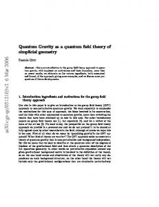
Figure 1: Sketch of sets of maps. a) The cone P of positive maps includes the cone CP of completely positive maps and its subcone CP containing the superpositive maps, dual to P. Trace preserving maps belong to the cross–section of the cones with an affine plane of dimension N 4 − N 2 (and of codimension N 2 ), representing the condition TrB D = IA . b) The sets of trace preserving maps in another perspective. This is a complete picture for N = 2 since some of the cones coincide, namely P = D and T = SP . For N ≥ 3, the complete picture is more complicated, see Figure 3. To clarify the duality relations (13), (14) and the structure of the cone SP, we recall that Φ is positive iff DΦ is block positive, which – by definition – is equivalent to Φ(ρξ ) ≥ 0 for every matrix of the form ρξ := |ξihξ|, that is, for every rank one positive semi-definite matrix. In other words, for any ξ ∈ HA and for any η ∈ HB , 0 ≤ hΦ(|ξihξ|)η, ηiHS = Tr Φ(|ξihξ|) |ηihη| = Tr DΦ (ρξ ⊗ ρη ) = hDΦ , ρξ ⊗ ρη iHS where the first tracing takes place in HB (or MN ) and the other in HA ⊗ HB , or in MN 2 (and similarly for the two Hilbert-Schmidt scalar products). This is the same as saying that DΦ belongs to the cone of matrices that is dual to the separable cone (the cone generated by all ρξ ⊗ ρη = ρξ⊗η or, equivalently, by all products ρA ⊗ ρB of positive semi-definite matrices). By the bipolar theorem for cones, this is equivalent to the cone {DΦ : Φ ∈ SP} being exactly the separable cone. An alternative description of SP, which justifies the “entanglement breaking” terminology, is as follows: Φ is superpositive iff for every k the extended quantum map Φ ⊗ Ik maps positive semi-definitive matrices to (positive semi-definite) separable matrices, or states to separable states if Φ is trace preserving. 13

Sometimes (see, e.g., Appendix 6.2) it is useful to work with extended sets of maps such as the convex hulls of PNTP ∪ {0} or PNb ∪ {0}. For technical reasons, we find the latter one more useful; we will denote it by P E = PNE , and similarly for other cones. Here 0 denotes the “zero” map, which may be chosen as a reference point. Further, one may b b consider symmetrized sets such as CP sym = CP sym N , the convex hull of −CP ∪CP , where −CP b is the symmetric image of CP b with respect to 0. (Note that CP sym is also the convex hull of −CP E ∪ CP E , see Figure 2 below.) The advantage in using 0-symmetric sets is that, first, they often admit an interpretation as unit balls with respect to natural norms and, second, that symmetric convex bodies have been studied more extensively than general ones convex bodies.

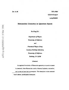
Figure 2: The set CP b of normalized quantum maps arises as a cross-section of the unbounded cone of CP maps with the hyperplane representing the condition Tr D = N. The set CP E of maps extended by the zero map is the convex hull of CP b ∪ {0}, while CP sym is the symmetrized set, the convex hull of −CP b ∪ CP b . CP sym may be identified with a ball in trace class norm, whose radius equals N. Analogous notation (and similar identifications) may be employed for other sets of maps including P, SP etc., or for abstract cones. We next introduce the auxiliary cone of completely co-positive (CcP) maps CcP = {Φ : T ◦ Φ ∈ CP},

where T : MN → MN is the transposition map (which is positive, but not completely positive for N > 1), and the cone T := CP ∩ CcP.

(15)

In terms of dynamical (Choi) matrices, DT ◦Φ is obtained from DΦ by transposing each block, i.e., by the partial transpose in the second system. This means that {DΦ : Φ ∈ T } is exactly PPT , the positive partial transpose cone (positive semi-definite matrices whose 14

partial transpose is also positive semi-definite). Since, as is easy to check, separable matrices are in PPT , it follows that SP ⊂ T ⊂ CP

(16)

For N = 2 the sets T and SP coincide, while for larger dimensions the inclusion SP ⊂ T is proper as shown in Figure 3.

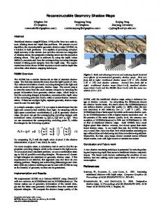
Figure 3: Sketch of sets of maps for N ≥ 3. a) The cone P of positive maps includes a sequence of nested subcones: the cone D of decomposable maps, CP of completely positive maps, T of maps which extended by identity impose positive partial transpose, and the cone SP of superpositive maps. b) The sequence of nested subsets of the compact set of positive trace preserving maps. Similarly to superpositive maps, there is an alternative description of T in the language of extended quantum maps: Φ ∈ T iff Φ ⊗ Ik is PPT inducing for any size k of the extension, i.e., for any state ρ acting on the bipartite system its image, ρ′ = Φ ⊗ I(ρ) ∈ PPT . [The necessity of the latter condition follows by noticing that the partial transpose of ρ′ equals (T ⊗ I)ρ′ = (T ◦ Φ ⊗ I)ρ, which is positive semidefinite due to T ◦ Φ being CP.] A quantum map Φ is called decomposable, if it may be expressed as a sum of a CP map Ψ1 and a another CP map Ψ2 composed with the transposition T , Φ = Ψ1 + T ◦ Ψ 2

(17)

or, equivalently, as a sum of a CP map and a CcP map. In other words, the cone D of decomposable maps is defined by D := CP + CcP (the Minkowski sum). Since the transposition preserves positivity, D ⊂ P. It is known [31, 32] that every one-qubit positive map is decomposable, so the sets P2 and D2 coincide. 15

However, already for N = 3 there exist positive, non–decomposable maps [33], so D3 forms a proper subset of P3 – see Figure 3. It follows from the identity (Φ, T ◦ Ψ) = (T ◦ Φ, Ψ) valid for all Φ, Ψ that CcP ∗ = CcP. Accordingly, the dual cone D ∗ verifies D ∗ = (CP + CcP)∗ = CP ∗ ∩ CcP ∗ = CP ∩ CcP = T

(18)

This is a special case of the identity (C1 + C2 )∗ = C1∗ ∩ C2∗ (the Minkowski sum) valid for any two convex cones C1 , C2 . It now follows by the bipolar theorem that D = T ∗.

(19)

As SP ⊂ T ⊂ CP by (16), it follows by duality that CP ⊂ D ⊂ P.

3.2

Bases of cones and duality; the inradii and the outradii. The symmetrized sets

We now return to the analysis of bases of cones of matrices, as defined in section 2.3. As was to be expected, natural set-theoretic and algebraic operations on cones induce analogous operations on bases of cones. Sometimes this is trivial as in (C1 ∩C2 )b = C1b ∩C2b , in other cases simple: (C1 + C2 )b = conv(C1b ∪ C2b ), where conv stands for the convex hull. What is more interesting and somewhat surprising is that also duality of cones carries over to precise duality of bases in the following sense. Lemma 1 Let V be a real Hilbert space, C ⊂ V a closed convex cone and let e ∈ V be a unit vector such that e ∈ C ∩ C ∗ . Set V b := {x ∈ V : hx, ei = 1} and let and C b = C ∩ V b and (C ∗ )b = C ∗ ∩ V b be the corresponding bases of C and C ∗ . Then (C ∗ )b := C ∗ ∩ V b = {y ∈ V b : ∀x ∈ C b h−(y − e), x − ei ≤ 1}.

(20)

In other words, if we think of V b as a vector space with the origin at e, and of C b and (C ∗ )b as subsets of that vector space, then (C ∗ )b = −(C b )◦ . Recall that for abstract cones C ⊂ V, the dual cone C ∗ is defined (cf. (11)) via C ∗ := {x ∈ V : ∀ y ∈ C hx, yi ≥ 0}. 16

This elementary Lemma seems to be a folklore result, but does not appear in standard references for convexity (the best source we were pointed to after consulting specialists was Exercise 6, §3.4 of [34]). However, once stated, the Lemma is straightforward to prove. If hx, ei = hy, ei = 1, then h−(y − e), x − ei = −hy, xi + 1 and so the condition from (20) can be restated as ∀x ∈ C b − hy, xi + 1 ≤ 1 ⇔ ∀x ∈ C b hy, xi ≥ 0. Since under our hypotheses C b generates C, the latter condition is equivalent to hy, xi ≥ 0 for all x ∈ C, i.e., to y ∈ C ∗ , as required. Let us now return to our more concrete setting of V = Msa d (endowed with the Hilbert-Schmidt scalar product) and e = Id /d1/2 . Even more specifically, we will consider V = Msa N 2 , identified via the Choi-Jamiolkowski isomorphism with the space of Hermicity preserving quantum maps on MN , and the cones that we defined in prior section. Note that the quantum map associated to e = IN 2 /N is the so-called “completely depolarising map,” which is usually denoted by Φ∗ and whose action is described by Φ∗ (M) = (N −1 Tr M) IN . The duality relations for cones (12), (13), (14) and (18), (19) combined with Lemma 1 imply now Corollary 2 We have the following duality relations for the bases of cones (CP b )◦ = −CP b , (SP b )◦ = −P b , (P b )◦ = −SP b (D b )◦ = −T b , (T b )◦ = −D b ,

(21)

where both the polarity and the negative signs refer to the vector structure in H b = {Φ : Tr DΦ = Tr Φ(IN ) = N} with Φ∗ as the origin. In other words, we have for example D b = {Φ ∈ H b : ∀Ψ ∈ T b (−(Φ − Φ∗ ), (Ψ − Φ∗ )) ≤ 1}. While the duality relations for cones described in the preceding subsection are rather well known, the duality for bases in the present generality appears to be a new observation. When combined with standard results from convex geometry, most notably Santal´o and inverse Santal´o inequalities [35, 36] (see below), and other tools of geometric functional analysis, it allows for relating volumes of bases of cones to those of the dual cones, and ultimately for asymptotically precise estimates of these volumes and of volumes of the corresponding sets of trace preserving maps. Let us also note here one immediate but interesting (and presumably known) consequence of the duality relations. 17

b Corollary 3 For each of the sets CP bN , SP bN , PNb , DN and TNb , the Euclidean (i.e., Hilbert2 −1/2 Schmidt) in-radius is (N − 1) and the Euclidean out-radius is (N 2 − 1)1/2 .

We observe first that, for each of the above sets, Φ∗ is the only element that is invariant under isometries of the set. Accordingly, it is enough to restrict attention to HilbertSchmidt balls centered at Φ∗ . For CP bN , the assertion is just a p reflection of the elementary fact that Mtot contains a Hilbert-Schmidt ball of radius 1/ d(d − 1) centered at the d p maximally mixed state ρ∗ , and that the distance from ρ∗ to pure states is 1 − 1/d. For sep SP bN , it is a consequence of equality of in-radii of Mtot N 2 and MN 2 (in the bivariate case) established in [13] (the out-radius of the latter is of course attained on pure separable states). It then follows that the in- and out-radii must be the same for the intermediate set TNb . Finally, since the out-radius of K ◦ is the reciprocal of the in-radius of K (and b vice versa), we deduce the assertion for PNb and DN via (21). It is curious to note that the statement about the out-radius of PNb is equivalent – via simple geometric arguments – to the following fact (which a posteriori is true) 2 2 If M = (Mjk )N j,k=1 is a block-positive matrix, then Tr (M ) ≤ (Tr M) .

It would be nice to have a simple direct proof of the above inequality, as it would yield (via Lemma 1 and (21)) an alternate derivation of the result from [13] concerning the in-radius of the set of separable states in the bivariate case. Similarly, the best (i.e., the smallest) constant R in the inclusion CP b − Φ∗ ⊂ R (SP b − Φ∗ ) is the same as the best constant in P b − Φ∗ ⊂ R (CP b − Φ∗ ). It has been shown in [13] that the optimal R satisfies N 2 /2 + 1 ≤ R ≤ N 2 − 1. [The upper bound follows just from the formulae for the inradius of SP b and the outradius of CP b (or, equivalently, Msep , Mtot ).] Again, there could be a more direct elementary argument. TP TP TP TP are Remark 4 The Euclidean inradii and outradii of CP TP N , SP N , PN , DN and TN b 2 −1/2 2 1/2 the same as for the larger C -type sets, i.e., (N − 1) and (N − 1) .

As pointed out in the arguments following the statement of Corollary 3, while the fact that the inradii and outradii of all sets in that Corollary are identical is nontrivial, there is no mystery about at least some of the maps (or directions) that witness them. In the language of the sets of states (i.e., matrices with trace one normalization) such witnesses are, for outradii pure states, and universal witnesses that work for all five sets 18

are pure separable states. By duality (i.e., Lemma 1), direction that witness inradii (for all sets) are obtained by reflecting a pure separable state with respect to the maximally mixed state ρ∗ . In the language of quantum maps purity (i.e., the Choi matrix being of rank one) corresponds to the map being of the form ρ → v † ρv (Kraus rank one), and the trace preserving condition is then equivalent to v being unitary. If that unitary is separable (i.e., a tensor product of two unitaries acting on the first and second system), the corresponding pure state will be separable. This means that universal witnesses of outradii of C b -type sets exist also in the smaller set by the trace preserving condition (5), i.e., inside the C TP -type sets. Since condition (5) defines an affine subspace, the “opposite” directions giving witnesses to the inradii also belong there. An alternative use of duality considerations involves symmetrized sets (cf. Figure 2). If C ⊂ V is a cone and C b its base, we define C sym := conv(−C b ∪ C b ); the minus sign referring now to the symmetric image with respect to 0. If, as earlier, e is the distinguished point of C ∩ C ∗ defining C b and (C ∗ )b , then (C sym )◦ = (e − C ∗ ) ∩ (−e + C ∗ ),

(22)

where the polarity has now the standard meaning (i.e., inside the entire space V and with respect to the origin). In other words, the polar of C sym is the order interval [−e, e], in the sense of the order induced by the cone C ∗ . The advantages of this approach is that we find ourselves in the category of centrally symmetric convex sets, which is better understood than that of general convex sets, and that frequently the object in question (C sym and its polar) have natural functional analysis interpretation as balls in natural normed spaces. One disadvantage is that in place of one very simple operation (symmetric image with respect to e) we have two elementary and manageable, but somewhat nontrivial operations (symmetrization and passing to order intervals). We postpone the discussion of (22) and related issues to the Appendix.

3.3

Volume radii and duality: Santal´ o and inverse Santal´ o inequalities

The classical Santal´o inequality [35] asserts that if K ⊂ Rm is a 0-symmetric convex body

2 and K ◦ its polar body, then vol(K) vol(K ◦ ) ≤ vol B2m or, in other words vrad(K) vrad(K◦ ) ≤ 1.

(23)

Moreover, the inequality holds also for not-necessarily-symmetric convex sets after an appropriate translation, in particular if the origin is the centroid of K or of K ◦ , a condition that will be satisfied for all sets we will consider in what follow. Even more interestingly, there is a converse inequality [36], usually called “the inverse Santal´o inequality,” vrad(K) vrad(K◦ ) ≥ c 19

(24)

for some universal numerical constant c > 0, independent of the convex body K (symmetric or not) and, most notably, of its dimension m. The inequalities (23), (24) together imply that, under some natural hypotheses (which are verified in most of cases of interest), the volume radii of a convex body and of its polar are approximately (i.e., up to a multiplicative universal numerical constant) reciprocal. By Lemma 1, the same is true for the base of a cone and that of the dual cone. This observation reduces, roughly by a factor of 2, the amount of work needed to determine the asymptotic behavior of volume radii of, say, sets from the third column of Table 1. We note, however, that since, at present, there are no good estimates for the constant c from (24) if K is not symmetric, it is often more efficient to revisit arguments from [14, 16] which allow to estimate volume radii of polar bodies without resorting to the inverse Santal´o inequality. (An argument yielding reasonable value of c for symmetric bodies was recently given in [37].)

20

4

Volume estimates: precise statements and approximate arguments

The results stated in section 3 allow us, in combination with known facts, to determine the asymptotic orders (as N → ∞) for the volume radii (and hence reasonable estimates for the volumes) of bases of all cones of quantum maps discussed up to this point. Our goal is slightly more ambitious; we want to find not just the asymptotic order of each quantity, but also establish inequalities valid in every fixed dimension and involving explicit fairly sharp numerical constants. Specifically, we will show the following Theorem 5 We have the following inequalities, valid for all N, and the following asymptotic relations

(i) 21 ≤ vrad CP bN ≤
1, limN →∞ vrad CP bN = e−1/4 ≈ 0.779 (ii) 14 N 1/2 ≤ vrad PNb ≤ 6N 1/2
b SP ≤ 4N −1/2 (iii) 16 N −1/2 ≤ vrad N

vrad TNb vrad TNb 1/4 1 e
≤ 1,
(iv) 4 ≤ ≤ lim inf N 2 vrad CP b vrad CP b N N

b b vrad DN vrad DN
≤ 8, lim supN
≤ 2e1/4 (v) 1 ≤ b b vrad CP N

vrad CP N

Remarks : (a) Estimates on volume radii listed in Table 2 are either identical to the corresponding inequalities stated above, or follow by the same argument. b (b) Since the asymptotic orders of the volume radii of the families CP bN , TNb and DN are the same, we chose – for greater transparence – to compare the volume radii of the two latter sets to that of CP bN in (iv) and (v), rather than give separate estimates for each of these quantities. (c) It is an interesting open problem α <
1

whether there exists a universal constantPPT b b such that vrad TN ≤ α vrad CP N for all N > 2 or, equivalently, “is vol MN 2 ≤
4 αN vol Mtot for some α < 1 and all N > 2?” Analogous question may be asked about 2 N

b comparing vrad DN and vrad CP bN . Inquiries to similar effect can be found in the literature [10, 38]. (d) It is likely that the asymptotic bound 2e1/4 in (v) holds actually all N. Indeed,
for −1/4 b there is a strong numerical evidence that the estimate vrad CP N ≥ e from (i) is valid for all N and not just in the limit. (In view of the explicit character of the formula (10) this issue shouldn’t be too difficult to resolve.) Should
that be the case, the next step b would be to carefully analyze the dependence of vrad DN on N given by the arguments presented in this paper. Since the bases of cones, whose volume radii are described by Theorem 5, are effectively homothetic images, with ratio N, of the corresponding sets of trace one matrices 21

(see Table 1 and the formulae that follow it), some of the inequalities/relations of Theorem 5 follow from known estimates for the volumes of various sets of states, particularly if we do not insist on obtaining “good” numerical constants that are included in the statements. For example, the estimates in statement (iii) are contained in Theorem 1 from [16]; one obtains the constants 16 and 4 by going over the proof of that Theorem specified to bilateral systems. Similarly, the statement (iv) is (essentially) a version of Theorem

PPT 4 from [16] which asserts that, in the present language, vrad MN 2 /vrad Mtot N 2 ≥ c0 for some constant c0 > 0 independent of the dimension N (the upper estimate with con−1/4 stant 1 is trivial). However, the argument from [16] yields only c0 = 81 and e 4 for the asymptotic lower bound. Next, the asymptotic relation in (i) follows from the explicit formula (10); see the comments following (10). Presumably, the estimates in (i) can also be derived from (10), but there are more elementary arguments. For a simple derivation of the lower bound from the classical Rogers-Shephard inequality [39] see [14], section II. And here is an apparently new proof of the upper bound: combine the duality results of the preceding section, specifically the identification (CP b )◦ = −CP b from (21), with the Santal´o inequality (23) to obtain




2 1 ≥ vrad CP b vrad (CP b )◦ = vrad CP b vrad − CP b = vrad CP b ,

as required. We recall that, in the context of (21), the operations ◦ and − take place in the space H b of quantum maps verifying Tr DΦ = N, with Φ∗ thought of as the origin; note that Φ∗ is the centroid of CP b and so (23) with K = CP b indeed does apply in that setting. Arguments parallel to the last one lead to versions of the remaining statements with some universal constants. For example, the identification (SP b )◦ = −P b combined with the Santal´o inequality (23) and its inverse (24) leads to

1 ≥ vrad SP b vrad P b ≥ c, where c is the (universal) constant
from (24). Combining the above
inequality
with (iii) we obtain 4c N 1/2 ≤ vrad PNb ≤ 6N 1/2 . Similarly, 1 ≥ vrad T b vrad D
b ≥ c vrad D b

N
≤ 32 combined with (the already shown version of) (iv) and with (i) implies vrad CP b N
b vrad DN
≤ 4e3/4 . As the constants in Theorem 5 are not meant to be and lim supN b

vrad CP N

optimal, we relegate the somewhat more involved (but still based on classical facts) arguments yielding them to Appendix 6.1.

The inequalities of Theorem 5 compare volumes of bases of cones, that is, sets of maps Φ normalized by the condition that the trace of DΦ , the corresponding Choi (or 22

dynamical) matrix, is N (or Tr Φ(IN ) = N). [Of course, any other normalization – most notably Tr DΦ = 1 leading to sets of states – would work just as well for comparing volumes provided we were consistent.] However, if we want to study quantum operations, i.e., trace-preserving quantum maps (or, similarly, unital maps), then – as explained in the previous sections – the corresponding constraints are stronger than just normalization by trace: in each case we are looking at an N 2 -codimensional section of the cone as opposed to the 1-codimensional base. However, in either case the codimension is much smaller than the dimension, which is N 4 − N 2 . The following technical result will imply that then, under relatively mild additional assumptions assuring that the base of the cone is reasonably balanced (which will be the case for all the cones we studied), the volume radius of the section will be very close to that of the entire base. Proposition 6 Let K be a convex body in an m-dimensional Euclidean space with centroid at a, and let H be a k-dimensional affine subspace passing through a. Let r = rK and R = RK be the in-radius and out-radius of K. Then 

vrad(K) R−

m−k m

b(m, k)

 mk

≤ vrad(K ∩ H) ≤

volm (B2m ) where b(m, k) := volk (B2k )volm−k (B2m−k ) 

 m1

vrad(K) r −

m−k m

  m1 ! mk m , b(m, k) k (25)

.

The proof of the Proposition is relegated to Appendix 6.3; now we explain its consequences. First, let us analyze the parameters that appear √ in (25). By Corallary 3, √ for all bases of cones that we consider here we have r = 1/ d − 1 and R = d − 1, where d = N 2 . Next, we have m = d2 − 1 = N 4 − 1, k = d2 − d = N 4 − N 2 and 1 m − k = d − 1 = N 2 − 1, in particular m = 1 + N12 = 1 + 1d and m−k = N 21+1 = d+1 . k m  m1  (related to the Beta function) Further, the quantity b(m, k) = Γ(k/2+1)Γ((m−k)/2+1) Γ(m/2+1) √ is easily shown to satisfy 1/ 2 < b(m, k) < 1 (for our values of m, k it is actually
1 m m N N )). Similarly, 1 ≤ ) for our values of ≤ 2 for all k, m and 1 + O( log 1 − O( log 2 N k N2 m, k. Consequently, if vrad(K) is subexponential in d (in our applications it is a low power of N, hence of d), then vrad(K ∩ H)/vrad(K) → 1 as N → ∞. This leads to Theorem 7 We have the following asymptotic relations
−1/4 (i) limN →∞ vrad CP TP N
= e
TP TP vrad PN vrad PN 1 (ii) 4 ≤ lim inf N N 1/2 ≤ lim supN N 1/2 ≤ 6 23

(iii)

1 6

(iv)

e1/4 2

(v)

≤ lim inf N

vrad SP TP N

≤ lim inf N

lim supN




≤ lim supN

N −1/2
vrad TNTP vrad CP b N

vrad SP TP N N −1/2




≤4






≤ 2e1/4 b

TP vrad DN

vrad CP N

Upper and lower bounds in the spirit of Theorem 5 (i.e., valid for all N) can be likewise obtained. The reader may wonder why we perform our initial analysis on bases of cones rather than working directly with the smaller sets of trace preserving maps. The reason for this is two-fold. First, the bases being homothetic to various sets of states, any information about them is at the same time more readily available and interesting by itself. Second, while we do have – as a consequence of Lemma 1 – nice duality relations between bases of cones, similar results for sets of trace preserving maps are just not true. As a demonstration of that phenomenon we show in Appendix 6.4 that, in contrast to the bases CP b , the sets CP TP are very far from being self-dual in the sense of (21).

5

Conclusions

We derived tight explicit bounds for the effective radius (in the sense of Hilbert-Schmidt volume), or volume radius, of the set of quantum operations acting on density matrices of size N, and for other convex sets of trace preserving maps acting such matrices such as positive, decomposable, PPT inducing or superpositive maps. The novelty of our approach depends on systematic use of duality to derive quantitative estimates, and on technical tools, some of which are not very familiar even in convex analysis. Since the volume radii of the sets of trace preserving maps that are positive display a different dependendce on the dimensionality than those of the smaller set of decomposable maps, the ratio of the volumes of the latter and the former set tends rapidly to 0 as the dimension increases. In other words, a generic positive trace preserving map is not decomposable and, a fortiori, not completely positive. Thus we were able to prove a stronger statement than the one advertised in the title of the paper. Similarly, a generic PPT inducing quantum operation (and, a fortiori, a generic quantum operation) is not superpositive. Analogous relations (some of which were known) exist between the sets of states related to those of maps via the Jamiolkowski isomorphism. Acknowledgements: We enjoyed inspiring discussions with I. Bengtsson, F. Benatti, V. Cappellini and H–J. Sommers. We acknowledge financial support from the Polish Ministry of Science and Information Technology under the grant DFG-SFB/38/2007, from

24

the National Science Foundation (U.S.A.), and from the European Research Projects SCALA and PHD.

25

6 6.1

Appendices Better constants in Theorem 5: mean width, Urysohn inequality and related tools

The arguments given in the preceding section did not yield the asserted values of the 1/4 constant 14 in part (ii), the constants e 2 and 14 in part (iv), and the constants 8 and 2e1/4 in part (v) of Theorem 5. We will now present the somewhat more involved line of reasoning that does yield these constants. The following concepts will be helpful in our analysis. If K ⊂ Rm is a convex body containing the origin in its interior, one defines the gauge of K via kxkK := inf{t ≥ 0 : x ∈ tK}. Roughly, kxkK is the norm, for which K is the unit ball, except that there is no symmetry requirement. Next, the mean width of K (or, more precisely, the mean half-width) is defined by Z Z w(K) :=

S m−1

kxkK ◦ dx =

maxhx, yidx

S m−1 y∈K

(integration with respect to the normalized Lebesgue measure on S m−1 ). A classical result known as Urysohn’s inequality (see, e.g., [41]) asserts then that vrad(K) ≤ w(K).

(26)

A companion inequality, which is even more elementary, is vrad(K) ≥ w(K ◦ )−1 .

(27)

The proof of (27) is based on expressing the volume as an integral in polar coordinates and R
1/m R then using twice H¨older inequality: vrad(K) = S m−1 kxk−m ≥ S m−1 kxk−1 K dx K dx ≥
−1 R kxkK dx = w(K ◦ )−1 . S m−1

b Applying (26) in our setting of the N 4 − 1-dimensional space H b and for K = DN , we obtain b b vrad(DN ) ≤ w(DN ) = w(conv(CP bN ∪ CcPNb )) ≤ w(CP bN + CcPNb ) = 2w(CP bN ) ≤ 4, (28)

because w(·) commutes with the Minkowski addition (of sets), and because w(CP bN ) = w(CcPNb ) ≤ 2. The latter is a consequence of similar estimates for the set of all states (which is equivalent to CP bN up to a homothety), see [14, 16]. (We note that while the limit relation w(CP bN ) → 2 as N → ∞ follows easily from well-known facts about random matrices, the estimate valid for all N requires finer arguments such as those presented in 26

appendices of [14]). Combining the above estimate with part (i) of Theorem 3 we obtain the upper estimate in part (v) with the asserted constant 8. b The same bound w(DN ) ≤ 4 combined with (27) (applied this time with K = TNb ) and with part (i) leads to the lower bound 14 in part (iv). To obtain the asymptotic bounds from part (iv) and (v) with the required constants e1/4 b and 2e1/4 we argue similarly, but instead of the universal estimate w(DN ) ≤ 4 we 2 b use a tighter asymptotic bound lim supN w(DN ) ≤ 2 This bound is a consequence of classical isoperimetric inequalities and the measure concentration phenomenon that they induce (see, e.g., [40]): a Lipschitz function on S m−1 is strongly R concentrated around its mean. In particular, if the out-radius of K is at most R, then S m−1 |kxkK ◦ − w(K)| dx = O(R/m1/2 ). If K = CP bN or CcPNb , then, by Corollary 3, R = (N 2 − 1)1/2 while m = N 4 − 1, hence R/m1/2 = (N 2 + 1)−1/2 < N −1 . It is then an elementary exercise to show that Z   b w(DN ) = max kxk(CP bN )◦ , kxk(CcPNb )◦ dx S m−1
≤ max w(CP bN ), w(CcPNb ) + O(N −1 ) ≤ 2 + O(N −1 ), b whence lim supN w(DN ) ≤ 2, as required. Universal (as opposed to asymptotic) upper b bounds on vrad(DN ) better than 4 obtained in (28) can also be derived this way, most efficiently by converting spherical integrals to Gaussian integrals and using the Gaussian isoperimetric inequality. (This would also improve somewhat the bounds 41 and 8 in parts (iv) and (v), but we will not pursue this direction here as the payoff doesn’t seem to justify the effort.) Finally, to obtain the lower bound on vrad(PNb ) from part (ii) of the Theorem, we note that the upper bound 4N −1/2 for vrad(SP bN ) (stated in part (iii)) was de facto (see [16]) deduced from the stronger estimate w(SP bN ) ≤ 4N −1/2 . It then remains to apply (27) and the duality between PNb and SP bN .

6.2

Symmetrized bodies and order intervals

We will now analyze the polar of the symmetrized body C sym . Recall the notation of section 3.2: V is a real Hilbert space, C ⊂ V a closed convex cone, C ∗ the dual cone. Next, e ∈ C ∩ C ∗ is a unit vector, V b := {x ∈ V : hx, ei = 1} is an affine subspace of V and C b = C ∩ V b is the base of the cone C. Finally, the symmetrized body is defined as C sym := conv(−C b ∪ C b ); the minus sign referring to the symmetric image with respect to 0. An important point, following from classical results [39, 44] and explained in Appendix C of [14], is that under mild assumptions which are satisfied for all the cones we consider, the volume radii of C b and of C sym differ by a factor smaller than 2. 27

Our main assertion (equation (22) in section 3.2) is that (C sym )◦ = (e − C ∗ ) ∩ (−e + C ∗ ), where the polarity has the standard meaning (i.e., inside the entire space V and with respect to the origin). That is, y ∈ (C sym )◦ iff both y + e and e − y are in C ∗ or, in other words, iff y belongs to [−e, e], the order interval in the sense of the order induced by
the ∗ b sym b b cone C . For example, if we want to investigate P and P = conv −P ∪ P , we may specify the framework above to C = P, obtaining

(P sym )◦ = − Φ∗ + SP ∩ Φ∗ − SP . To prove the assertion, denote V − := {x ∈ V : hx, ei ≤ 1} (one of the half-spaces determined by V b ) and C E = C ∩ V − (cf. Figure 2 in section 3). Then
C sym = conv(−C b ∪ C b ) = conv −C E ∪ C E .

Hence, using standard rules for polar operations (see, e.g., [41]),
◦
◦ (C sym )◦ = − C E ∩ C E .

Next,

CE


◦

= C ∩V−


◦


= conv (V − )◦ ∪ C ◦ = conv ((−∞, 1] · e ∪ −C ∗ ) = e − C ∗ ,

where the bar stands for the closure. Combining this with the preceding formula and again using the standard rules gives (C sym )◦ = (e − C ∗ ) ∩ (−e + C ∗ ) or the intersection of two cones with vertices at e and −e. Clearly this does not equal (C ∗ )sym except in dimension 1. However, the two bodies are closely related. For example, if e is the point of symmetry of C b , then (C ∗ )sym is a cylinder with the base (C ∗ )b and the axis [−e, e], while (C sym )◦ is a union of two cones whose common base is (C ∗ )b − e, the central section of the cylinder, and the vertices are −e and e. The two bodies only differ in one dimension; if thought of as unit balls with respect to the corresponding norms, the two norms coincide on the hyperspace V0 := {x ∈ V : hx, ei = 0} and on the complementary one-dimensional space Re, but on the entire space we have in the first case the direct sum in the ℓ∞ sense, while in the second case in the ℓ1 sense. If the base C b is non-symmetric, the situation is more complicated. For example, the section V0 ∩ (C sym )◦ is congruent to the intersection of (C ∗ )b with its symmetric image with respect to e, but (see [42]) the volume radii of the two bodies are comparable if, for example, e is the only point that is fixed under isometries of (C ∗ )b (as is the case in all our applications), or just the centroid of (C ∗ )b . 28

6.3

Proof of Proposition 2: for “balanced” cones, C b and C TP have comparable volume radius

We may assume that a = 0 (otherwise consider K − a). By hypothesis, we have then rB2m ⊂ K ⊂ RB2m ,

(29)

where B2m is the m-dimensional unit Euclidean ball. For a subspace E, denote by PE the orthogonal projection onto E. Then (see [42, 43]), volm (K) ≤ volk (K ∩ H) vols (PH ⊥ K),

(30)

where s = m − k and H ⊥ is the m − k-dimensional space orthogonal to the k-dimensional subspace H. Therefore volm (K) volk (K ∩ H) vols (PH ⊥ K) volk (B2k )vols (B2s ) ≤ volm (B2m ) vols (B2s ) volm (B2m ) volk (B2k ) Hence, using (29), vrad(K)m ≤ vrad(K ∩ H)k Rs

volk (B2k ) vols (B2s ) , volm (B2m )

which is the first inequality in (25). For the second inequality, we start with the even more classical result (see [44] or [45]; same notation as (30))  −1 m volk (K ∩ H) vols (PH ⊥ K), volm (K) ≥ k

(31)

which doesn’t even require that H passes through the centroid of K. As above, this can be rewritten in terms of volume radii as   volk (B2k ) vols (B2s ) m vrad(K)m ≥ vrad(K ∩ H)k r s , k vold (B2m ) which is the second inequality in (25).

6.4

“No duality” for CP TP N

The purpose of this Appendix is to show that, in contrast to the bases CP b , the sets CP TP are very far from being self-dual in the sense of (21), that is, that the polar of CP TP inside the space defined by the trace preserving condition (5) considered as a vector space with Φ∗ as the origin is quite different from the reflection of CP TP with respect to Φ∗ . 29

Generally, if K ⊂ Rm is a convex body containing the origin in its interior and H ⊂ Rm is a vector subspace, K ◦ ∩ H is always contained in the polar of K ∩ H inside H, and the discrepancy between the two (i.e., the smallest constant λ ≥ 1 such that the polar of K ∩ H is contained in λ(K ◦ ∩ H)) is the same as the discrepancy between K ∩ H and the orthogonal projection of K onto H. That discrepancy is also equal to the maximal ratio between maxhu, xi and max hu, yi (32) x∈K

y∈K∩H

over nonzero vectors u ∈ H. In our case K = CP bN and K ∩ H = CP TP N . As a vector space, H may be identified with maps whose dynamical matrix has partial trace equal to 0. We will argue in the language of dynamical (Choi) matrices considered as “flat” block matrices. In these terms, membership in H is equivalent to each block being of trace 0. We will choose as u the block matrix whose 11-th block is U = E11 − N −1 IN and the remaining blocks are 0. Further, we will choose as x the matrix whose 11-th block is X = NE11 and the remaining blocks are 0; then the scalar product corresponding to hu, xi is tr(UX) = N − 1. On the other hand, if Y is the 11-th block of the Choi matrix of any element of CP TP N , then Y is a state and so the scalar product corresponding to hu, yi is tr(UY ) = tr(E11 Y ) −N −1 trY ≤ trY − N −1 trY = 1 − N −1 . Accordingly, the discrepancy between the two maxima in (32) is at least (N − 1)/(1 − N −1 ) = N.

6.5

Volume radius of the set of trace non increasing maps

We want to determine the asymptotic order of the volume radius of the set of all completely postive, trace non increasing maps Φ : MN → MN i.e. the set := {Φ ∈ CP N : Tr Φ(ρ) ≤ Tr ρ for all ρ ≥ 0}. CP TNI N As pointed out earlier, an exact formula for that volume was very recently found (independently from this work and by a different method) in [30]. However, an argument using the approach of this paper is conceptually very simple and so we include it. We have Proposition 8 We have, for all N, eN


2 5/2 −N

≤

vol

CP TP N




vol CP TNI N




× vol {M ∈ MN : 0 ≤ M ≤ IN }


≤ N −N

2 /2

(33)


To derive estimates on vol CP TNI from the Proposition, one needs to use the readily N available information on the two factors in the denominator of the middle term of (33). First, the asymptotic order of the volume radius of CP TP N was determined in Theorem 30

7(i). Next, the set A := {M ∈ MN : 0 ≤ M ≤ IN } is a ball of radius 1/2 (in the operator norm) centered at IN /2, √ given by √ and so its volume radius admits easy bounds the in- and outradius: 1/2 and N /2 (actually a much tighter lower bound N /4 can be obtained via a slight modification of the argument from Theorem 5(i), see Appendix 6.1, but for our purposes the trivial bounds suffice). A straighforward calculation leads then to Corollary 9
lim vrad CP TNI = e−1/4 . N

N →∞

The key point is that in order to calculate the volume radius we need to raise the volume 2 to the power 1/N 4 . Thus the factors such as (e N 5/2 )−N on the left hand side of (33) N are inconsequential since it leads to an expression of the form 1 − O( log ). For the N2 same reason, the effects of vol(A) and of the b(m, k)-type factor, which also enters the calculation (cf. Proposition 6 and the comments following it), tend to 0 as N → ∞.

For the proof of Proposition 8 we note first that CP TNI is canonically isometric to the N set of subunital maps CP SU N := {Φ ∈ CP : Φ(IN ) ≤ IN }.

In what follows we will work with the latter set. The isometry, which assigns to Φ : MN → MN the dual (in the linear algebra, or Banach space sense) map Φ∗ , sends CP TP N SU to the set of unital maps CP U := {Φ ∈ CP : Φ(I ) = I }. The set CP admits a N N N N N natural fibration: with every M ∈ A, we may associate FM = {Φ ∈ CP : Φ(IN ) = M};

(34)

in particular FIN = CP U N . In the language P of Choi (dynamical) matrices the equality from (34) translates to trB DΦ = M, or to j Djj = M if we think of DΦ as a block matrix
DΦ = (Djk ) = PΦ(Ejk ) . Since all fibers FM are parallel to the subspace N defined by trB DΦ = 0 (or j Djj = 0), one can express the volume as an integral vol

CP TNI N




= vol 2

CP SU N




=N

−N 2 /2

Z

A


vol FM dM

(35)

The reason for the factor N −N /2 is that while the fibration is naturally parametrized by the elements of A, the projection of FM onto N ⊥ is actually the map ρ → N −1 tr(ρ)M, whose Choi matrix is N −1 IN ⊗ M (or a block matrix whose all diagonal blocks are M/N and off-diagonal blocks are 0). Now, the Hilbert-Schmidt norm of N −1 IN is N −1/2 , and ⊥ is isometric to N −1/2 A. so the projection of CP SU N onto N The second
inequality in
consequence of (35) and the
(33) is now
an immediate TP U bound vol FM ≤ vol FIN = vol CP N = vol CP N , valid for all M ∈ A, which 31

in turn follows, e.g., from FM being the image of FIN under the contraction gM : Φ(·) → 1 1 M 2 Φ(·)M
2 . (On the level of dynamical matrices, the action of gM is given by DΦ → 1 1 1
1 2 2 IN ⊗M DΦ IN ⊗M
or, in the language of block matrices, by (Djk ) → (M 2 Djk M 2 ).) The fact that gM FIN ⊂ FM is obvious from the definition; surjectivity for invertible −1 M’s follows by considering the inverse gM = gM −1 , and for singular M’s by looking at invertible approximants. For the first inequality in (33) we may use (31) with K = CP SU N and the section K ∩ U −1/2 H = CP N . As pointed out earlier, the set P
H K = P A, and
N ⊥ is thens isometric to N m m it remains to use the elementary bound k = s ≤ (em/s) . A alternative argument is to restrict the integration in (35) to {M : tIN ≤ M ≤ IN }, which is a ball in the −1 operator norm of radius (1 − t)/2, then use the fact that for such M the function cgM is a contraction, and finally optimize over t ∈ (0, 1). This approach allows in fact to express the Jacobian of gM in terms of eigenvalues of M and, subsequently, to express the ratio under consideration as a multiple integral over [0, 1]N , but we will not pursue this path further.

References [1] M. Adelman, J. V. Corbett and C. A. Hurst, The geometry of state space. Found. Phys. 23, 211 (1993). [2] M. Horodecki, P. Horodecki and R. Horodecki, Separability of mixed states: necessary and sufficient conditions. Phys. Lett. A 223, 1 (1996). [3] Arvind, K. S. Mallesh and N. Mukunda, A generalized Pancharatnam geometric phase formula for three-level quantum systems. J. Phys. A 30, 2417 (1997). [4] D. C. Brody and L. P. Hughston, Geometric quantum mechanics, J. Geom. Phys., 38, 19 (2001). [5] E. Ercolessi, G. Marmo, G. Morandi, and N. Mukunda, Geometry of mixed states and degeneracy structure of geometric phases for multi–level quantum systems. Int. J. Mod. Phys. A 16, 5007 (2001). ˙ [6] K. Zyczkowski and H.-J. Sommers, Hilbert-Schmidt volume of the set of mixed quantum states. J. Phys. A 36, 10115 (2003). [7] J. Grabowski, G. Marmo and M. Ku´s, Geometry of quantum systems: density states and entanglement. J. Phys. A 38, 10217-10244 (2005). [8] R. F. Werner, Quantum states with Einstein-Podolsky-Rosen correlations admitting a hidden-variable model. Phys. Rev. A 40, 4277 (1989).

32

[9] M. A. Nielsen and I. L. Chuang, Quantum Computation and Quantum Information, Cambridge University Press, Cambridge, 2000. ˙ [10] K. Zyczkowski, P. Horodecki, A. Sanpera and M. Lewenstein, Volume of the set of separable states. Phys. Rev. A 58, 883 (1998). [11] S. L. Braunstein, C. M. Caves, R. Jozsa, N. Linden, S. Popescu, and R. Schack, Separability of very noisy mixed states and implications for NMR quantum computing. Phys. Rev. Lett. 83, 1054 (1999). ˙ [12] K. Zyczkowski, Volume of the set of separable states II. Phys. Rev. A 60, 3496 (1999). [13] L. Gurvits and H. Barnum, Largest separable balls around the maximally mixed bipartite quantum state. Phys. Rev. A 66, 062311 (2002). [14] S. Szarek, Volume of separable states is super-doubly-exponentially small in the number of qubits. Phys. Rev. A 72 032304 (2005); arXiv.org e-print quant-ph/0310061. [15] P. B. Slater, Silver mean conjectures for 15–d volumes and 14–d hyperareas of the separable two–qubit systems. J. Geom. Phys. 53, 74 (2005). [16] G. Aubrun and S. J. Szarek, Tensor products of convex sets and the volume of separable states on N qudits. Phys. Rev. A 73, 022109 (2006); arXiv.org e-print quant-ph/0503221 [17] R. Hildebrand, Entangled states close to the maximally mixed state, Phys. Rev. A 75 062330 (2007) [18] M. Lewenstein and A. Sanpera, Separability and entanglement of composite quantum systems. Phys. Rev. Lett., 80, 2261 (1998). [19] A. Sanpera, R. Tarrach, and G. Vidal, Local description of quantum inseparability. Phys. Rev. A 58, 826 (1998). ˙ [20] M. Ku´s and K Zyczkowski, Geometry of entangled states. Phys. Rev. A 63, 032307 (2001). ˙ [21] S. Szarek, I. Bengtsson and K. Zyczkowski, On the structure of the body of states with positive partial transpose. J. Phys. A 39 L119-L126 (2006). [22] R. Clifton and H. Halvorson, Bipartite mixed states of infinite–dimensional systems are generically nonseparable, Phys. Rev. A 61, 012108 (2000). [23] A. Jamiolkowski, Linear transformations which preserve trace and positive semidefiniteness of operators. Rep. Math. Phys. 3, 275 (1972). ˙ [24] K. Zyczkowski and I. Bengtsson, On duality between quantum states and quantum maps. Open Syst. Inf. Dyn. 11, 3-42 (2004)

33

[25] M. B. Ruskai and S. Szarek and E. Werner, An Analysis of completely–positive trace– preserving maps on 2 × 2 Matrices. Linear Algebra Appl., 347, 159 (2002). ˙ [26] I. Bengtsson and K. Zyczkowski, Geometry of Quantum States, Cambridge University Press, Cambridge, 2006. [27] T. Ando, Cones and norms in the tensor product of matrix spaces. Linear Algebra Appl. 379, 3 (2004). [28] E. C. G. Sudarshan, P. M. Mathews and J. Rau, Stochastic dynamics of quantum– mechanical systems. Phys. Rev. 121, 920 (1961). [29] M.-D. Choi, Completely positive linear maps on complex matrices. Linear Alg. Appl. 10, 285 (1975). ˙ [30] V. Cappellini, H.-J. Sommers and K. Zyczkowski Subnormalized states and tracenonincreasing maps. J. Math. Phys. 48, 052110 (2007). [31] E. Størmer, Positive linear maps of operator algebras. Acta Math. 110, 233 (1962). [32] S. L. Woronowicz, Nonextendible positive maps. Commun. Math. Phys. 51, 243 (1976). [33] M.-D. Choi, Positive semidefinite biquadratic forms. Linear Alg. Appl. 12, 95 (1975). [34] Branko Gr¨ unbaum, Convex polytopes. Second edition. Prepared and with a preface by Volker Kaibel, Victor Klee and G¨ unter M. Ziegler. Graduate Texts in Mathematics, 221. Springer-Verlag, New York, 2003. [35] L. A. Santal´ o, An affine invariant for convex bodies of n-dimensional space. (Spanish) Portugaliae Math. 8, 155 (1949). [36] J. Bourgain and V. Milman, New volume ratio properties for convex symmetric bodies in Rn . Invent. Math. 88, 319 (1987). [37] G. Kuperberg, From the Mahler conjecture to Gauss linking integrals; arxiv.org e-print math/0610904 [38] M. Horodecki, P. Horodecki and R. Horodecki, Mixed-State Entanglement and Quantum Communication. In Quantum Information, Springer Tracts in Modern Physics 173, 151 Springer Verlag, Berlin-Heidelberg 2001. [39] C. A. Rogers and G. C. Shephard, The difference body of a convex body. Arch. Math. 8, 220 (1957). [40] V. D. Milman and G. Schechtman, Asymptotic theory of finite dimensional normed spaces. With an appendix by M. Gromov. Lecture Notes Math. 1200, Springer Verlag, Berlin-New York, 1986.

34

[41] R. Schneider Convex bodies: The Brunn-Minkowski Theory. Cambridge University Press, 1993. [42] J. E. Spingarn, An inequality for sections and projections of a convex set. Proc. Amer. Math. Soc. 118, 1219 (1993). [43] V. D. Milman and A. Pajor, Entropy and asymptotic geometry of non-symmetric convex bodies. Adv. Math. 152, 314 (2000). [44] C. A. Rogers and G. C. Shephard, Convex bodies associated with a given convex body. J. London Math. Soc. 33, 270 (1958). [45] G. D. Chakerian, Inequalities for the Difference Body of a Convex Body. Proc. Amer. Math. Soc. 18 No. 5, 879 (1967).

35