research to provide a comprehensive and easily understood analysis ofgeostatistics' manner of modeling and methods. The traditional geostatistical tool, the ...
Ecological .\lonographs 62(2). 1992. pp. 277-314 6 1992 by the Ecological Society of America
GEOSTATISTICAL TOOLS FOR MODELING AND INTERPRETING ECOLOGICAL SPATIAL DEPENDENCE1 RICHARD E. ROSSI Department of Applied Earth Sciences, Stanford C’niversity, Stanford, California 94305-2225 C’SA
DAVIDJ. MULLA Department of Agronomy and Soils, Washington State C’niversity, Pullman, Washington 99164-6420 USA
A N D R G. ~ . JOURNEL Department of Applied Earth Sciences, Stanford University, Stanford, California 94305-2225 USA
ELDONH. FRANZ Program in Environmental Science and Regional Planning, Washington State University, Pullman, Washington 99164-4430 C’SA
Abstract. Geostatistics brings to ecology novel tools for the interpretation of spatial patterns of organisms, of the numerous environmental components with which they interact, and of the joint spatial dependence between organisms and their environment. The purpose of this paper is to use data from the ecological literature as well as from original research to provide a comprehensive and easily understood analysis ofgeostatistics’ manner of modeling and methods. The traditional geostatistical tool, the variogram, a tool that is beginning to be used in ecology, is shown to provide an incomplete and misleading summary of spatial pattern when local means and variances change. Use of the non-ergodic covariance and correlogram provides a more effective description of lag-to-lag spatial dependence because the changing local means and variances are accounted for. Indicator transformations capture the spatial patterns of nominal ecological variables like gene frequencies and the presence/absence of an organism and of subgroups of a population like large or small individuals. Robust variogram measures are shown to be useful in data sets that contain many data outliers. Appropriate removal of outliers reveals latent spatial dependence and patterns. Cross-variograms, cross-covariances, and cross-correlograms define the joint spatial dependence between co-occurring organisms. The results of all of these analyses bring new insights into the spatial relations of organisms in their environment. Key words: Balanus; Diabrotica; Dyschirius; geostatistical modeling theory and methods: h-scattergram: indicator variogram: Mus; non-ergodic correlogram and cross-correlogram: non-ergodic covariance and cross-covariance; Pterostichus; spatial dependence of organisms in environment; spatial outlier: spatial pattern: variogram and cross-variogram.
INTRODUCTION What is geostatistics and why use it? Statistical procedures are often used to organize and summarize data so that meaningful inferences can be made about phenomena ofinterest. Commonly in ecology the foundation of such an inference is a statistical test like a t , F, and x2 test or a procedure like an analysis of variance (ANOVA). These tools are convenient and easy to implement, but they generally assume that any one datum is independent of all other data and that the data are distributed identically. Are these assumptions tenable for most ecological investigations? We submit that assuming spatial dependence is more practical and realistic, since what we identify as ecological phenomena involves a recognition of correlation.
’ Manuscript received 10 September 1990; revised 25 May 1991; accepted 28 May 1991.
Spatial and temporal dependence or continuity should be readily apparent to the ecologist: vegetation species and densities are generally different on north-facing vs. south-facing slopes; grasshoppers (Orthoptera) are more dense during hot, dry periods; and in greenhouse experiments plants are routinely rotated to eliminate microclimatic and microenvironmental (space-time) effects. Ecological analysis normally includes investigations of the dispersion and patterns in association between different species at different places and at different times (Pielou 1977)-patterns that reflect spatial dependence, not independence. Indeed, the very definitions of ecology, like “the study of the natural environment, particularly the interrelationships between organisms and thir surroundings” (Ricklefs 1973) and “the scientific study of the relationships between organisms and their environments” (McNaughton and Wolf 1973), or of key concepts, such as levels of or-
RICHARD E. ROSS1 ET AL.
278
ji,
Ecological Monographs Vol. 62. No. 2
trayed in Figs. 1 and 2. One class of statistical tools concentrates on the statistical modeling of spatial dependence and is known as “geostatistics.” Geostatistics is a branch of applied statistics that focuses on the detection, modeling, and estimation of spatial patterns. Although the mainstay of developments in this field have come from geology and mining, as will be seen shortly (The tools of geostatistics applied. . . : The variogram: a bivariate, statistical model, below), the development and use of one key technique has an old, if largely forgotten, history in forestry (cf. MatCrn 1960).
There is more to geostatistics than the variogram and kriging FIG. 1. Perspective plot of Hengeveld’s (1979) summer collection of the carabid Dyschirius globosus on a reclaimed polder. Separation distance between intersection points on the sampling grid is 40 m.
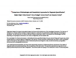
ganization (Odum 1975), presuppose spatial and temporal dependence. Spatial dependence is particularly important in an analysis of spatially varying organism distributions and environmental variables, yet many traditional statistical measures tend to ignore it. Consider Hengeveld’s (1979) report of the spatial distribution of a carabid beetle, Dyschirius globosus, on an 800 x 400 m reclaimed Netherland polder. Five pitfall traps were arranged in a hexagon and centered at each node of a 2 1 x 12 sampling grid spaced 40 m apart, and the numbers of D. globosus caught during the months AprilAugust were reported. A perspective plot (Fig. 1) of the data reveals a marked concentration of the organism around the center of the sampling space. In addition, two areas near the center of this concentration display particularly large values. Overall, the value at any one location is similar to the values at neighboring locations. Consider another very different distribution, one distributed over a sampling space of equivalent dimensions to Hengeveld’s design (Fig. 2). Unlike the spatially continuous D. globosus distribution, this new pattern contains disjoint large, medium, and small concentrations throughout the sampling space, with no readily apparent pattern. Nevertheless, because this new grid is merely a randomized version of the D. globosus data, both grids contain precisely the same sample size and values. Thus, each has exactly the same frequency distribution and univariate statistics (Fig. 3). A statistical analysis or test based solely on measures such as mean, variance, coefficient of variation, or frequency distribution cannot capture their obvious differences. A different organizing and summarizing tool is needed- one that characterizes the degree of spatial dependence, or lack thereof, between sampling locations. There are many techniques that can distinguish between the obviously different spatial distributions por-
Recently ecologists have begun to implement two geostatistical techniques: variography, which is one way to model spatial dependence, and kriging, which provides estimates for unrecorded locations. Philips (1 985) uses variograms and their fractal representation to monitor shoreline erosion rates in New Jersey’s Delaware Bay to test the hypothesis that a common reed accelerated the erosion. Robertson (1 987) provides two examples of geostatistical applications: ( 1) temporal variability of the density of cell counts for a Rhodomonas sp. in a lake epilimnion and (2) spatial variability of soil mineral nitrogen in a Michigan old-field. Kemp et al. (1989) use statewide grasshopper (Orthoptera: Acrididae) counts in three regions of Montana to create, with kriging, region-specific macroscale hazard maps of grasshopper densities. Schotzko and O’Keeffe (1989) model the spatial variability of the Lygus bug Lygus hesperus in an agricultural field and then use kriging to map that organism’s density. These studies point to increased interest in geostatistical methods in ecology, but they leave important considerations, explanations, a n d caveats unaddressed. One missing feature is a description of the underlying theory and assumptions of geostatistics.
FIG. 2. Perspective plot of Hengeveld’s (1979) carabid beetle data, which were presented in Fig. 1; here they have been rearranged randomly over the same sampling space.
June 1992
GEOSTATISTICAL TOOLS FOR ECOLOGY
These foundations must be appreciated in order that the transfer of the techniques be accomplished effectively and correctly. Moreover, the mainstay of geostatistical literature can present an often-daunting array of jargon and mathematical and statistical formulas. Our goal is to present a primarily intuitive appreciation of these foundations-one that contains a minimum of mathematical and statistical nomenclature, but one that is rich in ecological examples and yet theoretically rigorous. More importantly, ecology stands to benefit greatly by a presentation of modeling and estimation techniques not utilized in the aforementioned papers. As we show below, unusually large and small data (i.e., outliers) can greatly affect the interpretation of spatial dependence when using the variogram. It is critical, therefore, to be aware of methods for their identification and to have an understanding of the circumstances in which their removal is valid. Additionally, we provide examples of a type of variogram, known as an “indicator variogram,” that can be used to model the spatial dependence between nominal ecological variables such as gene frequencies. We also show how indicator variograms can be used to model the spatial dependence of a particular size class of the organism’s total sample set. This provides a potent new dimension to the traditional variogram because it permits identification of the spatial patterns of ecologically meaningful subgroups within a population, like the youngest or smallest individuals vs. the oldest or largest ones. Other very powerful modeling tools for ecological analysis, ones absent from the above-mentioned papers, model the joint spatial dependence between two co-occurring species or between an organism and a known or suspected influential component of its environment. These techniques strike at the heart ofwhat is ecology. Finally, and most importantly, using ecological examples we demonstrate that the variogram modeling tool used in the above papers may actually provide an incomplete image of spatial pattern. This is because the variogram is affected strongly by small-scale or local mean and variance differences. Alternative spatial modeling tools are described and illustrated, ones that are more resistant to small-scale data effects. These alternative tools not only uncover spatial dependence more accurately, they can also uncover spatial patterns undetected by the variogram. We use data from the botanical and zoological literature to describe and illustrate new geostatistical methods. Using already-published data is helpful because a comparison between the findings and the results of geostatistical and conventional analyses can hasten comprehension of new terms and analytic procedures and improve interpretations. In this paper we describe the underlying rationale and procedures of geostatistics, develop its analytical tools, and delve into some allied techniques that are
279
\UTl3€’
Mean S t a i d a f d Deviarion CoefficieTt of Variation Skewress Uin,mum Medial Maximum humbe. of 0 ’ s
252 28.54 58.04 2.03 2,87 0
2 334
a1
0
shown to be particularly helpful in ecological analysis. The emphasis is on how the analytical tools can be used to interpret plant and animal spatial patterns, regardless of whether the models are ever used in a kriging procedure to estimate values for unrecorded locations. Readers interested in a fully developed, introductory text on geostatistical theory and practice are strongly encouraged to see Isaaks and Srivastava’s ( 1 989) recent work. For its clarity, rigor, and rich illustrations, there is no finer one. Concise introductory works that use examples from soil science and agronomy are Vieira et al. (1 983), Burgess and Webster ( 1 980), and Webster (1985). More complete texts by Journel and Huijbregts (1978), David (1977, 1988), and Rendu(l981) require a working knowledge of matrix algebra as well as integral calculus, and use mining examples exclusively. Recent short lessons (40 pages) by Journel(l989) provide an updated review of modem geostatistics, but do not present any case studies. Ecology has produced a large and long-lived literature on spatial patterns and their interpretation. It is not our intention to review these works since they are most likely already familiar to most ecologists and excellent reviews are readily available. Our purpose is to develop the geostatistical approach, an approach that is probably less familiar and one that, until recently, has been used sparingly. Prominent among the many extant ecological works are Greig-Smith’s (1983) excellent treatment of botanical spatial patterns and Taylor’s (1984) review of methods for diagnosing insect distributions. Pielou’s (1 977) text offers a developed assessment of frequently used spatial analysis tools. Cliff and Ord (1 973), Ripley (1 98 1, 1988), and Diggle’s (1983) books are important sources of methods for
RICHARD E. ROSS1 ET AL.
280
D. g l o b o s u s
1,
,
lo[ ,
:,
8
- Summer , 1,O , 1: , l p , 1,6 ,
1,8 ,
7 10 8
c 8
6
.D
4
x
’!
2
2
OO
A
_u
2
4
6
8
10
12
14
16
18
28
P. coerulescens - Summer 2
0
4
6
8
12
10
14
16
18
20
Ecological Monographs Vol. 62. No. 2
shaw and Ford (1 984) can be consulted for interesting applications. Both geostatistics and time series utilize the covariance function (defined below-see Eq. l), but time series focuses on Fourier transforms of the data, and thus calculations are performed in frequency domain. This transformation places practical restrictions on the input data and on subsequent interpretations. In the time-series method input data are usually continuous (i.e., rather than categorical) and are arrayed on a regular grid. Sparse or irregularly spaced data do not present a problem for geostatistics. The time-series approach is designed to recognize periodic components of the spatial phenomenon. Geostatistics is capable of uncovering the periodic as well as the often non-periodic nature of ecological parameters. On a practical level, because time-series’ calculations are performed in frequency domain and then back-transformed, calculations can often be complex and tedious. Geostatistical operations are performed in the original data domain and are therefore easier to both calculate and interpret. GEOSTATISTICAL PROCEDURE IN ECOLOGICAL ANALYSIS
P. coerulescens
1
,
:,
8
,
1,O
,
1,2
- Fall
,
1,4 , 1 , 6 c , 2C, 10
,
f
X dimension
FIG.4. Contour plots ofbeetle counts in Hengeveld’s (1 979) summer collections of Dyschirius globosus and Pterostichus cnerulescens and the fall collection of P. coerulescens. Grid spacing is 40 m. as in Fig. 1.
sampling and analysis of spatial point patterns in ecology. Patil et al. (1 97 1a, 6, c), Cormack et al. (1 979), Cormack and Ord (1 979), Grassle et al. (1 979), Ord et al. (1979), and Orloci et al. (1979) provide comprehensive references and numerous examples of applications. An approach that is related to geostatistics, one that has been applied in ecology, is that of time series as applied to spatial patterns. Platt and Denman (1975) offer a clear review of the use of this technique in ecology, Shugart (1978) provides a good collection of papers on the topic, and Ford (1976), Ripley (1978), Ford and Renshaw (1 984), Renshaw (1 984), and Ren-
The fundamental m a x i m of geostatistics. -Before delving into examples, it is important to emphasize a fundamental precept of geostatistical analysis: geostatistics is never a replacement for sound ecological reasoning. This precept is true for any statistical procedure and may seem self evident, yet in practice it is frequently overlooked. No matter how compelling the result, to be credible a statistical or geostatistical finding must receive support from the data or, at a minimum, from ecological theory. All statistics corroborate or contradict; they cannot prove or disprove. Exploratory data analysis before geostatistics. -The first task in all geostatistical investigations is not at all geostatistics. Before computing any of the spatial statistics customarily associated with geostatistics, an exhaustive exploratory data analysis (or EDA) should be performed (Tukey 1977). An EDA involves computing traditional univariate and bivariate statistics, histograms, regression plots, and scattergrams. With multivariate data, an EDA may also include cluster analysis, principal component analysis, and an analysis of variance. Only after this initial foundation has been established should spatial statistics be entertained, because the results obtained from each step guide the kinds of analyses capable of producing meaningful results in the following steps. As an introduction, we now present the EDA highlights of four ecological data sets. These works will be used to demonstrate geostatistical methods. Data set 1: carabid beetle densities on a reclaimed polder Hengeveld’s (1 979) report of the distribution of Dyschirius globosus on a reclaimed polder has already been
28 1
GEOSTATISTICAL TOOLS FOR ECOLOGY
June 1992
partially introduced (see Introduction: What is geostatistics . . . above). Hengeveld also provides counts of another carabid species, Pterostichus coerulescens, captured during the same summer (April-August) period and for the following fall (September-October) period as well. Isarithmic maps of the counts reveal the summer areal distribution of P. coerulescens to be different from that of D. glcbosus (Fig. 4). The pattern of the distribution of P. coerulescens changes little between seasons, though there are many more beetles in the fall. P. coerulescens’ distribution displays a pronounced trend, one that is stronger and confined to a smaller portion of the whole sampling grid during the fall. Perspective and isarithmic plots of data permit quick appraisal of spatial features and trends, but they are not very efficient summaries. Moreover, given the nature or arrangement of the data, it may not always be practical or possible to compute such plots. In those instances, univariate and bivariate statistics and plots help to uncover important spatial features of the data. A useful univariate summary of data is a frequency table and its corresponding graph, the histogram. Frequency distributions are useful because they provide a description of the probability or likelihood associated with a given value. For example, in the histograms for both D. globosus (Fig. 3 ) and P. coerulescens (Figs. 5 and 6), the largest proportion of sampling locations contains the smallest number of beetles while the largest concentrations occur with the smallest frequency. These important features can be described by a summary statistic like “skewness.” Skewness refers to a histogram’s symmetry about the mean; the predominance of small or large data make a histogram asymmetric. The positive skew evident in the carabid beetle samples attest to their frequency distributions’ drawn-
kurroer Uean
252 270.36 271.61 Coef’icient o f V a r i c t i o n 1 .01 Skewpess 1.14 L1i n ’ r r L r r 0 L1e c i a -, 217 Ucximum 1414 \Lrn>er of 0 ’ s 6
St a -, c c r c 2ev i c :i o P
I
-
-
A-
3
530
1033
r r 1500
I
2330
’
2530
Beetles/Slte
FIG.5 . Frequency histogram and some summary statistics for Hengeveld’s (1 979) summer collection of the carabid
Pterostichus coerulescens.
I
r
40
4
kLm3er
Wean S t a - , d a r c Deviation Coefficient of Variation Skew-ess Minirrum Median W3XirrLrr
\urroer
of 0 s
252 401.72 509.14 1.27 1.34 0 140 2518 18
FIG.6. Frequency histogram and some summary statistics for Hengeveld’s (1979) fall collection of the carabid Pterostr-
chus coerulescens.
out lengths and asymmetric shapes about their means. Another useful statistic that expresses a histogram’s overall spread around its mean is the “coefficient of variation.” The coefficient of variation is simply the ratio of the sample standard deviation to its mean. Another constructive way to describe the carabid distributions is to analyze their bivariate distributions. Because bivariate statistics and plots characterize the relationships and dependencies between any two variables, they can yield a richer summary of the data than a univariate description can. Consider some bivariate scatter plots for D. globosus (Fig. 7). The top two graphs plot the sample numbers as a function of their X (long grid side) and Y (short grid side) locations, and the bottom left graph plots the beetle’s density as a function of the sum of the X and Y directions. These particular directions are chosen for demonstrative purposes only. Any linear combination of directions (i.e., a X b Y ) may be plotted in an attempt to reveal directional trends or discontinuities. When there are many data, or when samples are distributed in spatially distinct regions, quick visual appraisal of the raw data may not be possible. In such circumstances the researcher may have to plot multiple linear combinations in search of prominent trends and discontinuities. As is evident in the shape of the scatter of points in Fig. 7 , D. globosus’ distribution is clumped in the center of the X direction and favors the smaller-valued portion of the Y direction. Plot D compares the sample values between the two species and shows that areas of large concentrations of D. globosus correspond to areas where P. coerulescens densities are around 300 individuals/site. The linear strength of these bivariate relations is summarized using covariance and correlation coeffi-
+
400
A
3
Ecological Monographs Vol. 6 2 , No. 2
RICHARD E. ROSS1 ET AL.
282
x
2
300
-
B
300-
0 9 u
u
03
03
s'
200-
L
0 L
X
Y
dimension
??
300i 9 03
L
300\
All Data ( N =252):
t E
I
u
4001D
Ln
dimension
Covariance = 1673.8 = 0.107 P R =~ 0.621 ~ ~
300
Non-Zero Data ( N =171):
m
xn
Covariance =
p^ = -0.076
200
/5R0"k
u
2oo;
- 1310.03
= 0.138
03
s' E
100 L
a
Z
n E Z
0
5
10
15
20
25
30
35
X+Y dimension
0 0
400
800
1200
Number of P. coerulescens - Summer
FIG.7. Bivariate scatterplots that plot the number of Dyschirius globosus against their X direction value, their Y direction value, the sum of the X and Y direction values, and the number of Pterostichus coerulescens found at the same location and time of collection (data from Hengeveld 1979).
cients. The estimated covariance, 6,,, between two variables, u and v, is the average product of the differences between each variable and their respective means, m,, and m,:
where N is the total number of pairs of sample values (u,, v,). Eq. (1) may appear a bit peculiar when compared to the more traditional formulation of this statistic. Typically N - 1 is used as a denominator rather than simply N. The denominator N - 1 is theoretically justified when the data are independent- indepen-
dence across the u,, v, pairs. Geostatistics does not use this justification because it starts from the assumption of data correlation, correlation between pairs of spatially arrayed data. Also, formulae in most geostatistical references frequently do not distinguish between the parameter estimates and the true statistical parameters. To the practiced geostatistician, the context of the discussion is usually sufficient to differentiate the two. However, in keeping with the traditional convention, the present paper will denote estimates with a symbol. A covariance value depends on the units of measurement of both variables u and v. A unit-free or dimensionless measure is obtained by standardizing the covariance by the product of the two standard de''h"
GEOSTATISTICAL TOOLS FOR ECOLOGY
June 1992 AIi D a t a
N
3330,
-
Eovar o r c e
F,
~
O+Vk
0
Yor-Zero
Data
252 121,773
233 122,573
0 887 3 932
0 883 0 916
I
LL
2330
4
I
1230
Nu-nber
o4
P coerulescens
-
1600
Su-n-ne.
FIG. 8. Bivariate scatterplot that plots the numbers of Pterostichus coerulescens found dunng the fall collection vs. the number found during the summer collection (data from Hengeveld 1979).
viations. The resulting statistic is known as the estimated Pearson product-moment or the linear correlation coefficient:
The Pearson correlation coefficient measures how well one variable can be represented as a linear function of the other. This statistic can range from - 1 to + 1 depending on whether the variables are related linearly in a negative or positive manner; a score of - 1 corresponds to perfect negative linear correlation and + 1 to perfect positive linear correlation. A +0.107 correlation between the two beetles suggests a very low positive linear relationship exists between their densities (see Fig. 7). Nevertheless, the two variables u and v could be highly dependent without being linearly related, a classic example being: u = v2. A measure of monotonic dependence, whether linear or not, is the "Spearman rank correlation" (Davis 1986). The Spearman rank correlation is none other than the linear correlation coefficient of the data's ranks. For instance, sample u, has rank R,,,and is equal to 1 if it is the smallest value and N if it is the largest value of u. Similarly, the corresponding sample v, has rank R,!. The Spearman rank correlation coefficient is thus defined as:
u and v values, and sR,, and sR, are the standard deviations of the ranks of the u and v values. Notice that when comparing D. globosus and P. coerulescens densities, the Spearman correlation coefficient is different from the Pearson correlation coefficient. The small Pearson but large Spearman statistics suggest that the relationship between D. globosus and the co-occurring P. coerulescens beetle could be nonlinear. However, this comparison pairs locations where no beetles are present for one species with those where the other species does exist. Namelq, there are 8 1 D. globosus locations and 6 P. coerulescens locations where no beetles of the other species were present. Another way to analyze the data is to compare only those locations that actually contain both beetles. When these latter locations are analyzed, the Pearson statistic becomes -0.076 and the Spearman statistic an inconsequential 0.138. Thus, the relationship between the two co-occurring beetles is apparently neither linear nor monotonic. Consider the bivariate scatterplot and summary statistics for P. coerulescens between the summer and fall collections (Fig. 8). Even when the non-zero data locations are considered, there is a strong, positive, and linear relationship between the numbers of P. coerulescens in the summer and in the fall.
Data set 2: acorn barnacles, Balanus balanoides, on the side of a ship Kooijman ( 1 976) provides another example of an organism's spatial distribution using a grid count. A 10 x 10 grid, 0.75 x 0.75 m, was superimposed on the hull of a cutter docked in Scheveningen, Holland, and the acorn barnacles, Balanus balanoides, in each cell were counted. In all, 166 barnacles were counted in the sampling grid. A plot of the cell counts reveals four distinct areas of large density and no overali directional preferences (Fig. 9). As can be seen in the
' ;Ron&
=
N
283
0
1
2
3
4
5
5
7
5
9
(3) S R ~ R ,
where mRuand mR,are the means of the ranks of the
FIG. 9. Diagram of Kooijman's (1976) acorn barnacle (Balanus balanoides) grid-count data. Grid cells were ~ 7 . 5 x 7.5 cm.
RICHARD E. ROSS1 ET AL.
284 43 -
- 100 1.66
?.lo Me-icn Mc x , m J T, Num>e, 0'
'24 -1
, n
~
1
,
2
l 3
3 s
! 4
.27 1.59 0 1 9 35
l 5
6
I
7
,
9
I
I
9
'
3 0 ~ 1 o ce s / C e l l
FIG. 10. Frequency histogram and some summary statistics for Kooijman's (1976) data presented in Fig. 9.
histogram for these data (Fig. lo), > 60 of the 100 cells contain either one or no barnacles while two of the cells are populated with the largest (8 and 9) densities of barnacles. The large proportion of small or no barnacles is reflected in the distribution's strong positive skew. In a later work Kooijman (1979) sketches the outlines of all 166 barnacles within the sampling space, showing their relative size (Fig. 11). This new perspective on the data reveals that four distinct clusters are actually composed of mostly smaller barnacles. Alternatively, one can observe that the larger barnacles are distributed apparently more or less uniformly throughout the sampling area. To evaluate the potential significance of barnacle size and spatial pattern, these data were digitized using an ellipse as a model shape, and relative estimates were made of the barnacles' size (here, surface area). The histogram of barnacle size indicates that a large proportion of the total number are small barnacles, there is a nearly equal frequency of medium-sized individiials, and the largest barnacles comprise the smallest proportion of the total (Fig. 12). Barnacle size is, however, less variable overall than the cell counts (coefficients of variation, slm, are 0.78 for size vs. 1.27 for counts). As is readily seen in the raw data plot (Fig. 1 l), the distribution of various-sized barnacles does not appear to contain any strong, overall directional preference. The two renditions of the same acorn barnacle data underscore an important facet of ecological data analysis: the way the data are presented or summarized largely determines the resulting interpretation that can be made of that data. When just the barnacle cell numbers or densities are considered, four clusters are clearly evident (see Fig. 9), but there is no indication that the clusters are composed of primarily smaller, and pre-
Ecological Monographs Vol. 62, No. 2
sumably younger, barnacles. That observation is obvious when an actual sketch of the barnacles is considered (see Fig. 11). To the ecologist seeking an explanation for the spatial patterns of acorn barnacles, these age-size differences can be critical. When examining the spatial relations of ecological variables, other important considerations are the size, shape, and orientation of samples. In geostatistics these sample features are known as the "support" of the data. Support plays a major role in determining the kinds of statistical inferences that can be made toward understanding the phenomena of interest. For example, consider some summary statistics for the barnacles when the same sampling area is redefined as a 5 x 5, 15 x 15, 20 x 20, or a 25 x 25 grid of cells (Table 1). As the subareas over which the data are averaged decrease, the mean and variance also decrease, while skewness increases. As will be seen below (see The tools of geostatistics applied. . . :The multi-scaled spatial arrangement of B. balanoides . . . :The spatial dependence. . .), when geostatistical procedures are implemented to investigate the barnacle spatial patterns considering their size, diagnosis of spatial dependence is itself heavily dependent on the data support. While the raw data posting of barnacles is an explicit visual description, often it is important to know something of how variable a region is in relation to another and what the mean pattern or trends are. "Movingwindow" statistics help to provide this additional information. As the name implies, summary statistics are computed for successive and possibly overlapping subregions throughout the sampling space. Changes in window mean and variance as a function of location provide information about the patterns of local variability and the average size of the barnacles (Fig. 13). Notice how, overall, the cell means and variances tend to track one another. This tendency for the local means to be proportional to the local variances
0 c3
0 25
0.5c
3.75
FIG. 1 1. Plot showing the relative size and location of the surface areas occupied by Kooijman's (1 976) 166 acorn barnacles (after Kooijman 1979).
GEOSTATISTICAL TOOLS FOR ECOLOGY
June 1992
285
instance, consider the distribution of genotypes in a population; one can speak of the proportion of individuals in the population that contain a certain genotype, but normally there is no intrinsically meaningful continuous variable that can be associated with the presence of one genotype or another. One useful example is Selander’s (1 970) description of small-scale genetic variability of the house mouse, Mus musculus. Although genetic theory is concerned usually with genetic differences at the scale of continents, Selander showed distinct genetic variability at the scale of a few metres. Selander laid out a square grid ( ~ 0 . m 5 spacing) of
U nbe r 166 MecE 78 7.63 Stc-dard DevatioC 75 C o e f f ’ c ’ e n t o f V a r i a t oq Skew-ess 79 M ninJn 04 Med c n 7 22 N c x rrrn 2E 98 8”
;
3c
S;’-P-
Arec C c e - p l e d
i ” c
by 3 a r I o c es (TI-‘:
FIG. 12. Frequency histogram and some summary statistics for the estimated surface ares occupied by the individual acorn barnacles (data from Kooijman 1979). 65.13
can be appreciated quickly when the cell standard deviations are plotted as a function of their means (Fig. 14). In geostatistics, when the local means and standard deviations share a predictable relationship, the data are said to contain a “proportional effect.” Linear proportional effects, like the one depicted in Fig. 14, are common in lognormally distributed data (Isaaks and Srivastava 1989). As will be seen below ( T h e tools of geostatistics applied . . . : The multi-scaled spatial arrangement of B. balanoides . . . : The spatial dependence . . .), the presence of a proportional effect influences substantially the interpretations that can be made using a spatial dependence tool like the variogram.
Data set 3: small-scale genetic variability of house mice, Mus musculus, in a Texas chicken barn Ecologists frequently study phenomena that can only be characterized or are best described using names or nominal variables rather than numerical measures. For
10.29
0
?
2
3
4
5
6
7
8
9
FIG. 13. Moving-window statistics for estimates of the surface areas occupied by Kooijman’s (1 979) 166 barnacles, shown in Fig. 1 1, using the original support (a 10 x 10 array of cells each 7.5 cm on a side). The top number is the total number of barnacles, the middle number is the mean, and the bottom number is the variance of the estimated surface areas occupied by the barnacles in each cell. Blank cells contain 5 2 barnacles.
TABLE1. Summary statistics for Kooijman’s (1976, 1979) acorn barnacle counts after changing the data support (here, the resolution of the sampling scheme). Note that the actual area and the number of barnacles are the same; only the grid size changes. Number of cells _________~
~
Statistic
5 x 5
Mean Variance Standard deviation Coefficient of variation Skewness Minimum Median Maximum Cell size fm)
6.64 32.79 5.73 0.86 0.68 1 3.50 19
1.66 4.43 2.10 1.27 1.59 0 2 9
0.74 1.30 1.14 1.54 1.84 0 0
5
5
0.27 0.29 0.54 2.05 2.06 0 0 3
0.15
0.075
0.05
0.0375
0.03
10 x 10
15 x 15
20 x 20 0.42 0.57 0.76 1.82 2.33 0 0
25 x 25
286
RICHARD E. ROSS1 ET AL. '21r:ercep: = 1 48 S c z e = 3 46
5
i
=
3.57
-
I
I
1.,1 e c f I
"
"
'5
12
FIG.14. Plot ofthe cell standard deviationsvs. their means for the grid depicted in Fig, 13 showing evidence of a proportional effect. Note: only cells containing 2 3 barnacles are presented. Original data from Kooijman ( 1 979).
mouse traps in a 57 x 15 array in a chicken barn at Austin, Texas. In one night's trapping, 378 house mice were captured, and each was then tested for a common mammalian blood enzyme, esterase-3. The mice exhibited one of three traits or genotypes corresponding to the particular genetic makeup of the individual: homozygous medium, heterozygous, and homozygous slow (see Fig. 15). The designations "medium" and "slow" refer to the speed of the protein migration in the electrophoretic gel used to characterize the three different esterase-3 genotypes. In all, there were 51 homozygous medium (1 3.5% of total), 164 heterozy-
Ecological Monographs Vol. 62. No. 2
gous (43.4% of total), and 163 homozygous slow mice (43.1% of total). Selander plotted the distribution of mouse genotypes and drew contours by hand corresponding to major genotype zones (Fig. 15 presents Selander's raw data only). He explained the demonstrable heterogeneity as a result of mouse tribal behavior. Typically, one male dominates several females and several subordinate males. This social behavior, coupled with mouse territoriality and inbreeding, were suggested as mechanisms for the resulting small-scale genotype distribution. A few years after this original study, Sokal and Oden (1 978a, b) analyzed these data using a nearest-neighbor autocorrelation technique. They investigated three chess-like "moves" or combinations of directions, rook's, bishop's, and queen's, for contiguous sampling sites. They found significant positive autocorrelation between contiguous pairs Of mice with the homozygous medium gene and a significant negative autocorrelation between mice containing the two homozygous genotypes. Although they concede that their analysis displays no evidence for significant heterozygote-heterozygote pairings (i.e., pockets of homozygotes separated by heterozygotes), they suggest that such an arrangement might be expected theoretically.
Data set 4: adult northern corn rootworm, Diabrotica barberi, density and corn, Zea mays, root damage Our final data set is based on original field research by Jon Tollefson (personal communication) at Iowa State University concerning the interrelationship between the northern corn rootworm and Zea mays plants. Rootworm larvae feed exclusively on corn roots and
.....
00000
ooooo
H o m o z y g o J s MediJrn Heterozygous H o m o z y g o u s Slow
0
6-
-
0
Y
.-m n
o
80 0
o
88 08
0
0. 88
0 09: 0 88
8....8
0
0
. 0
8 8 . 088.0
808. 0 8 008
0
80
0
.0.
0 0 0 0 0 0 . 8 8 . 0 0 . . 0000 0 0 0
08
0 0
0
O . .
0 0.
0. 0 0 880.888 0 0 8 0 0 . . 08 0.. 0 0 0 0 8 .8.8 ...0.
88. 0.. 08 0 ..0. 088.0 0 0 00008 0 88 00008 08.8 0 0 0 88 80.808.. 88 3 2 .8.8 0. 80. 00 .0.008 0 0 80 0. 888. 0 0 8.808 0 0 .88. 888.8 0 0.. 808 0 0 0 0.... 0 0 0. 0. . 8 . 8 . 8 . . . . . 0 0 800.0. 80 0. 0 0 88.888 0. ....O 0 088.8. 8.8. 0 0 0 08 8 8 0 88.... 0 0. ..88 0. 0 0 - 00.8 8 8 88..8808088. 0 088.0 0 0 0. 0 0. 008 0 8 8 0 . 0 0 0 0. 8 8 0 0-
0.
0
....
-
-6
00 0
-3
-0
Distance (m) FIG. 15. Diagram of locations of the three esterase-3genotypes of captured Mus musculus individuals in a Texas chicken barn (after Selander 1970).
GEOSTATISTICAL TOOLS FOR ECOLOGY
June 1992
TABLE2. Summary statistics for J. Tollefson’s (personal communication) corn rootworm data. (Diabrotrca barberi larvae feed on Zea mays roots.) Number of beetleslplant
Number of locations
Percentage of total sites
0
13 113 48 55 43 272
4.8 41.5 17.7 20.2 15.8 100.0
1
2 3 24
can cause substantial economic loss (Chiang 1973). Surveying rootworm damage, however, requires that corn plants be extirpated, a labor-intensive, destructive procedure that also creates gaps in the crop canopy, which can hasten lodging. During the summer of 1988, Tollefson tested the unproven hypothesis that root damage is positively related to the density of recently matured beetles. Nine northwest Iowa counties were chosen randomly and, in all, 272 total corn fields were surveyed. At each sampling location the number of adult beetles and the severity of root damage were estimated. As a measure of rootworm density, an index was assigned to a location according to the number of beetles counted. A summary of beetle indices and their proportions is provided in Table 2. Similarly, a root-rating index was assigned to each location based upon the extent and severity of root damage. Descriptions of the root indices and the summary proportions are itemized in Table 3. A bivariate scatter plot of these two variables would not be very illuminating since both variables are indices, and thus there are only five possible values for the beetle rating and four for the root rating (one of which contains only one value). Given these circumstances, more revealing statistics are “conditional” statistics: histograms of beetle indices graphed for each root-index category (Fig. 16). Of the 50 sites having a root index of zero, 98% also have a beetle index of eiiher zero or one while only 2% score a beetle index of two. For the 190 sites having a root-rating index of one, 40.53% have a beetle rating of either zero or one, 24.2 1% scored a two, and 25.26% scored either a three
287
or four. At the 31 locations with a root index of two, none scored a beetle rating of zero or one, only 3.23% had a score of two, and the vast majority (96.77%) scored a three or four. Only one location manifested the largest root rating of three, but it also scored the largest beetle index of four. Apparently, there is a positive relationship between the root and beetle indices. The conditional histograms depicted in Fig. 16 make explicit the tendency for locations to have positively correlated beetle and root indices. Some summary statistics can mask this result. For instance, relating root rating to the beetle rating results in only a moderate 0.63 Pearson correlation coefficient. But the Spearman rank correlation coefficient is a much stronger 0.89. One explanation for the incongruous Pearson and Spearman correlation coefficients is that the relationship between beetle numbers and the severity of root damage is nonlinear, yet it is monotonic. Another possible reason for the discrepancy is that outliers (i.e., large values in one data set paired with small values in the other, or the converse) drastically reduces the point-to-point Pearson correlation between the two sets. This large-small or small-large data pairing is mitigated once the data’s ranks are considered. THETOOLSOF GEOSTATISTICS APPLIEDTO ECOLOGICAL PHENOMENA Now that the four ecological data sets have been introduced and a flavor for their spatial relations has been provided by plots and univariate and bivariate statistical analyses, we are ready to analyze their spatial continuity with more-advanced tools. Although univariate and bivariate measures provide useful summaries, they do not describe all the spatial features of data. Features such as the locations of extreme values, trends, or degree of continuity can be of major importance in understanding the ecology of an organism, but they cannot be derived completely from the tools and techniques utilized thus far. Spatial continuity measures quantify the relationship between the value of a variable at one location and the value of the same variable or another one at other locations. The basic idea of spatial continuity is simple and self-evident: on average, the closer two sampling points are to each other, the more likely it is that their values will be similar.
TABLE3. Root indices and summary proportions for J. Tollefson’s (personal communication) corn rootworm data. (Diabrotica barberi larvae feed on Zea mays roots.) Root index
0 1 2 3
Root condition No damage Visible feeding scars Minor loss of root structure Major loss of root structure
Number of locations
Percentage of total sites
Mean no. of beetledplant
50 190 31
18.4 69.8 11.4 0.4 100.0
0.86 2.02 3.71 4
1
272
288
RICHARD E. ROSS1 ET AL
Root Index
=
Ecological Monographs Vol. 62, No. 2
0
(N=50)
7-
-
J
m 220011 1I I r h ,
I
-
,
1
0
i
i
j
i
- 0
O- 1 - 1 00
B e e t l e Index
1 2 3 B e e t e Index
4
4 4
5
Rgot Index = 3 ( N =1)
lO0l
O - 1 0
1 2 3 1 2 3 B e e t l e Index
6
i
e
i
7
5
B e e t e Index
FIG.16. Conditional histograms of adult Diabrotica barberi density indices for the four Zea mays root-rating categories (data from J. Tollefson, personal communication).
There is a wide and flexible variety of spatial continuity tools in geostatistics, among which the most useful are h-scatterplots, variograms, correlograms, and covariance measures. Using the four ecological data sets, we now explore how these tools quantify an organism attribute or environmental variable’s spatial patterns. Additionally, we see how the patterns of the interaction between an attribute of an organism and some component of its environment can also be quantified and interpreted. h-scatterplots. -In geostatistics the bold letter h is generally taken to represent some separation vector in space, one that has a direction and distance to it. When temporal phenomena are the focus of interest, h refers to a time interval. Often, however, the lag distance may refer to a scalar distance, an average over all directions, in which case we will use “h” rather than “h.” One way to portray the degree of spatial continuity at some lag distance h is to compute an h-scatterplot. An h-scatterplot is simply a plot of the pairs of all data values separated by a common lag. Consider four h-scatterplots for Hengeveld’s summer collection of the carabid beetle Pterostichus coerulescens (Fig. 17). Since the raw data are so strongly skewed, they were first uniform-rank transformed. A uniform-rank transform is performed easily by ranking
the data in ascending order and then dividing each rank by the total sample size. This new variable, u(x),has the advantage that it is distributed in the interval [0, 11, and each increment is constant. Consequently, in the resulting h-scattergram, neither the preponderating small values nor the small number of large ones are privileged visually. The four plots of Fig. 17 show all possible pairings of the 2 5 2 data separated by a lag of one, two, three, and four units, independently of direction, where each unit is the minimum sample spacing of 40 m. These plots depict all transformed values at all locations x, u(x),against all other values a distance h away, u(x + h). If two data separated by h are identical, then they would fall somewhere on the h-scatterplot’s 45” line. Since this is rarely the case, the plotted points instead define a scatter or “cloud” of points around the 45” line. Notice that the cloud of h = 1 scatterplot points is the narrowest of the four. With increasing distance the cloud becomes wider and more diffuse. This result is to be expected since the general idea of spatial continuity is that proximate data are, on average, more similar than those that are farther apart. In the h-scatterplot for lag distance one, note how one point [i.e., u ( x + h ) 2: 0.731 falls quite far from the 45” line when paired with smaller data. This means
GEOSTATISTICAL TOOLS FOR ECOLOGY
June 1992
'.O
1 1
289
....
Susoected
.. H 3
W
1 ---T-
0.2
0.4
0.'6
0.8
1.0
FIG.17. Omnidirectional h-scattergrams for lags one through four of Hengeveld's ( 1 979) summer collection of Pterostichus coerulescens. Carabid density counts were first uniform rank-transformed to eliminate the bias of the strongly skewed raw data.
that of all the h = 1 comparisons, this datum is most mlike its contiguous neighbors. This point corresponds to a location where 465 beetles were captured, but its eight contiguous neighboring data are 16, 80, 100, 264, 291, 297, 332, and 345 beetles. One may suspect, therefore, that this value is an outlier, a value so large as to be distinguished rightfully from its neighbors. If there are sound physical or ecological reasons (e.g., the number of carabid beetles at that location was incorrectly counted, an unusually large concentration of the beetle's favorite food occurred at this location, etc.), then the researcher is justified in removing the datum so as not to let this one uncharacteristic value influence the statistical interpretations that can be made of the carabid beetle's spatial continuity. Alternatively, thanks to the h-scatterplot, we now know that the 465 datum is more unlike its closest data than any other
datum. Determining the reasons for this large concentration could be a valuable aid toward understanding the ecology of P. coerulescens. It is important to recognize that although the count of 465 is most unlike its neighboring values at h = 1, and hence might be an outlier, at other lags it may be neither the most dissimilar nor an outlier. At h = 4, for instance, other data plot as far or farther from the 45" line. Therefore, whether or not a value is an outlier cannot be determined with reference to only one specific lag. Besides their ability to indicate possible outliers or misrecorded values, h-scatterplots may also signal the presence of distinct populations. Different populations with different spatial continuities will usually plot as distinct clouds or scatters of points. Such distinct modes may or may not appear on the raw histogram. If dis-
RICHARD E. ROSS1 ET AL.
290
Summary statistics for Pterostichus coerulescens’ TABLE 4. four h-scatterplots shown in Fig. 17.
h
Lag covanance (no. of beetles)2
Correlation coefficient
(no./cell)2
1 2 3 4
59 757 52 307 46 647 40 466
0.862 0.796 0.728 0.656
9817 15 175 21 083 27 413
6ooc
Moment
Ecological Monographs Vol. 6 2 . No. 2
1 I
of inertia
@’
-I Crete populations are suspected, the researcher should, data permitting, separate the distinct populations and analyze them separately for spatial continuity. Otherwise, an analysis on the mixture of populations may provide a misleading (i.e., merely average) portrait of the extant spatial relations. Another advantage of h-scatterplots is that their asymmetry about the 45” line can signal trends or differences in the local means and variance. In the graphs in Fig. 17, for example, note how the small u(x)values plot disproportionately more often on the u(x + h) side of the 45” line. This asymmetry corresponds to comparisons between locations with small densities and those having larger densities of beetles. We have already seen that P. coerulescens’ density reflects a strong trend (see Fig. 4), so this feature is reflected in the h-scatterplot. h-scatterplots are useful tools, but they fail to summarize precisely and succinctly spatial continuity. The degree of scatter or the size of the cloud in an h-scatterplot can be summarized using the covariance (Eq. 1) or the correlation coefficient (Eq. 2) measures. The first two columns of Table 4 itemize the covariance and correlation coefficients for each of the four lag distances for P. coerulescens. Both the covariance and the degree of correlation decrease with increasing lag distance, and thus, as suspected, the data are more dissimilar the farther apart they are. Another measure of spatial continuity, the “variogram,” is a traditional geostatistical tool. Its formulation is related to both spatial covariance and correlation functions, and it is also an effective summary of an h-scatterplot. Before delving into these relations, however, let us first explore an intuitive description of the variogram. The variogram: a bivariate, statistical model. -Consider again the carabid beetle distribution that shows a clear pattern (Fig. 1) and the same data rearranged in a random pattern (Fig. 2). The variogram is one method for distinguishing the obvious differences between these two spatial distributions. Like the spatial covariance and correlation functions, the variogram models the average degree of similarity between the values as a function of their separation distance. Journel (1 984b) describes an insightful method for understanding the variogram. His approach recognizes
1000-
o
ooooo P a t t e r r e d 3 a t a M+E R a n d o m 3 a t a
0
I
C
~
,
2
,
,
I
’
4
,
#
,
6
1
I
i0
8
12
Lcg 3’stcnce (40m J i ‘ t s )
FIG. 18. Omnidirectional variograms for the patterned spatial distribution shown as a perspective plot in Fig. 1 and the random spatial distribution shown similarly in Fig. 2. i.( h )is the estimated variogram value; the horizontal dashed line depicts the overall sample variance of both data sets. Original data from Hengeveld (1979); the grid spacing in the original data collection was 4 0 m.
the variogram as an effective summary of an h-scatterplot: each variogram value summarizes one h-scattergram. Half the average squared distance between all h-scatterplot points and the 45” line can be seen as the moment of inertia of the points about that line. That is, if x, and y, are the coordinates of one of the h-scatterplot points, then the moment of inertia for all N points is defined: Moment of inertia
=
.I
\
-
2N
(x,
-
yJ2.
(4)
!=,
The values for the moments of inertia for the four P. coerulescens h-scatterplots presented in Fig. 17 are itemized in Table 4 (third column), and are the variogram values for all directional combinations of pairs of points separated by exactly 1 , 2, 3, and 4 lags. A variogram function summarizes all h-scattergrams for all possible pairings of data:
where +(h) is the estimated semivariance value for lag h and N(h) is the number of pairs of points separated by h. Put another way, this new expression for the variance between a pair of points is the half- or semivariance, or as it is simply referred to in the geostatistical literature: the “variogram.” Variograms can be computed as either an average over all directions, in which case the lag measure is scalar, or specific to a particular direction, in which case the lag measure is a vector. Variograms computed from the data displayed in
June 1992
GEOSTATISTICAL TOOLS FOR ECOLOGY
Fig. 1 and Fig. 2 for all possible pairs of points over the sampling space are distinctly different (Fig. 18). For the random data all values are essentially the same, and thus the variogram appears nearly horizontal. The patterned data, on the other hand, produce a variogram that has small values for short lags, then increases with increasing distance, but levels off and even decreases after about lag nine. These features reflect the degree of spatial variability or, conversely, continuity in the data. Constant variogram values mean that, on average, the variance between values does not change with distance. Small variogram values at short lags correspond to data that are closer together and more alike or more spatially continuous. Conversely, large variogram values reflect data that are farther apart and more dissimilar or spatially discontinuous. Notice that the random pattern’s vanogram remains near the sample variance of 3369. A plot of these raw data demonstrated no detectable spatial continuity (see Fig. 2 ) , and this characteristic is reflected in the fairly constant variogram, one nearly equivalent to the overall sample variance. In this instance the sample variance suffices to summarize the spatial continuity at all lags. In contrast, the patterned data set’s variogram values summarize the degree of spatial variability evident at each particular lag distance. It should be pointed out that a variogram is a special type of model. Although a model is typically defined as a deterministic paradigm that explains or predicts, a variogram is a statistical model. It summarizes the samples’ two-point or bivariate relations, i.e., the average squared difference between samples aligned in a particular direction and separated by some common lag. This observed or experimental variogram is a descriptive statistical model for the particular realization of the phenomenon under study. Because our sampling is limited, we assume, therefore, that our experimental variogram is representative of the true variogram had our sampling been exhaustive. We have said that the variogram is a statistical model of spatial dependence. Traditionally, there are two types of spatial dependence: “structural” and “stochastic.” Structural spatial dependence refers to large-scale data trends and involves jointly several data locations. Stochastic spatial dependence refers to small scale correlation structures usually at distances smaller than the separation distance between two data locations. Although the distinction between the two types is scale dependent, the variogram models structural spatial dependence. Credit is usually given to Matheron (1963, 1965), Journel and Huijbregts (1978), and David (1977) among many others in the field of mining geology for demonstrating the variogram’s practical use. To be sure, their works have advanced the use of the variogram as a spatial-continuity measure. Nevertheless, some years before mining geologists took note of the advantages of the variogram, biomathematicians Matern
29 1
(1947) and Jowett ( 1 955) used a “serial variation function” identical to the variogram. Their application involved quantification of local or short-distance vs. longdistance variation and its effect on the proper design of sampling regimes. Matern (1 947) applied spatial correlation measures to the distribution of Swedish forests. Whittle’s (1 954, 1956, 1963) works, especially his 1963 text, foreshadowed much of the geostatistics that was later developed by Matheron and his associates in Fontainebleau, France. Some of the same can be said for Wold (1938), Kolmogorov (1941), Wiener (1949), Yaglom (1 957), Goldberger (1 962), and Gandin (1 963). But even these works were not among the oldest. Matern (1 960) relates that the Swedish forester Langsaeter used what is essentially the variogram to express variation in forest surveys as early as 1926. Now that the idea of a variogram and a bit of its biological heritage has been developed, let us re-examine this old tool using the four ecological data sets. In addition, we also explore some other related, but often more revealing and dependable, spatial-continuity tools. Most of the spatial-continuity tools will be presented using Hengeveld’s (1979) carabid beetle data. These data are best suited to introduce the tools because the spatial patterns of the carabids are readily apparent in the raw data plots (Fig. 4), so interpretation using these new tools is more quickly grasped. This will be a distinct advantage later when the spatial patterns of other organisms are investigated-organisms whose spatial patterns are not as visually obvious.
The spatial and temporal interrelationships of Dyschirius globosus and Pterostichus coerulescens Variography: the calculation and interpretation of variograms. -In Fig. 18 we saw how a variogram distinguishes between a patterned and a randomly distributed carabid beetle’s spatial distributions. Those quantifications of pattern were computed by considering all possible pairs of the 252 available data on D. globosus. In geostatistics such variograms are often called “omnidirectional” variograms since they are an average over all pairs of data no matter their orientation or direction from each other. We may inquire whether spatial continuity changes with direction or location over the sampling space. After all, the plots of both beetles’ distributions (Fig. 4) reveal different patterns in different regions and changes with direction. How can the variogram account for such obvious differences? Variograms can be computed for subregions of the sampling grid so long as there are a sufficient number of data. A geostatistical “rule of thumb” is that each lag class must be represented by at least 30-50 pairs of points (Journel and Huijbregts 1978). However, the greater the number of pairs of points, the greater the statistical reliability in each distance class. Directional variograms. -Variograms may also be calculated for specific directions. Assume that what we
292
RICHARD E. ROSS1 ET AL.
0:; 3
,
, i
,
I
,
4
Lcg ?'s:crce
I
,
,
a
13
( 4 3 r Jr'tsj
FIG. 19. Standardized directional variograms, with 22.5" increments and ? 1 1.25" tolerances. for the summer collection of Dyschirius globosus. Original data from Hengeveld (1 979).
have taken to be the X axis or long side of the carabid sampling space corresponds to the 0" direction (a standard to which we henceforth adhere). Since the carabid beetle data were collected on a regular square grid, computing pure 0" and 90" variograms is easy: only pairs of points that fall on the same row or column need be considered, and then all rows or columns are averaged. Likewise, pure 45"- and 135"-directional variograms could be computed by pairing data points that lie precisely in those directions. This scheme works well for data sampled on regular, square grids, but it would be difficult, and perhaps impossible, to implement precisely with irregularly spaced data. Moreover, even if the data were on a regular, square grid, limiting the pairing of data values to only those that align exactly along the same direction is unnecessarily restrictive. For example, say a value at location ( 0 , 0) i s paired with the one at location (10, 1). These two points are separated by a distance of only 10.05 which is very close to 10. However, they do not bclong to either the same row or column, nor do they fall along a common 45" or 135" diagonal. Still, the angle separating them is only 5.7". Clearly, if we compare values that fall within a specific tolerance around the required direction and distance, then points like ( 0 , 0) and (10, 1) can be paired legitimately without a loss of variogram specificity. In this way we may designate the spatial dependence for any combination of direction and tolerance for any sampling regime. Directional variograms for D. globosus, computed in 22.5" increments with a k 11.25" (non-overlapping) tolerance, reveal small differences in spatial continuity with direction (Fig. 19). Before we consider their subtle differences, however, two features of these plots need to be explained: (1) some directions have fewer points plotted than others, and (2) all of the variograms' val-
Ecological Monographs Vol. 62, No. 2
ues are standardized by dividing each by the total sample variance. Like the 30-50 pairs minimum rule of thumb, only half the total distance measured in any direction over the sampling space may be represented legitimately in a variogram. This restriction assures that all lag classes are truly representative of the sampling space, because lags larger than half the maximum distance compare only the edge points of a sampling region. Thus, the O",22.5", and 157.5" variograms contain values out to "lag 10 while the 67.5", 90°, and 112.5" variograms contain values out to only -lag six. Accordingly, subregion variograms for the carabid data would not be very meaningful since they would contain an insufficient number of points. Standardized variograms. -Since a variogram is a plot of half the average squared difference between data separated by about the same distance and oriented in about the same direction, different data will have different variograms. If the overall variability in values is large, then the variogram values will also be large. It would be useful to compare the spatial variability between the summer collections of P. coerulescens and D. globosus, but the sample variance for the P. coerulescens is nearly 22 times larger than that for D. globosus. Consequently, their variograms will be difficult to compare. One way to standardize their variograms is to divide each variogram value by the overall sample variance. This standardizes each plot so that a unit variogram value is equivalent to the sample variance. Standardizing their variograms allows meaningful spatial-dependence comparisons to be made between data with disparate measurement units and/or levels of spatial variability. Returning to Fig. 19, we can see that the slopes of the variograms for directions 45", 67.5", and 90" are less than for the other directions. This means that the rate of change in the density of D. globosus in these directions is smaller than for the other directions. This interpretation can be observed readily in the exhaustive map ofthe species (see Fig. 4): the isarithms extend farther into the sample space in the 45" to 90" directions. Conversely, this beetle's density reflects a faster rate of change in the other directions, a feature which corresponds to steeper slopes in the other directional variograms. Differences in spatial continuity with direction is known as "anisotropy," while similar spatial continuity with direction is known as "isotropy." The summer collection of P. coerulescens manifests distinct and dramatic anisotropy (Fig. 20). Most of the directional variograms are linear, but some, like the 135" and 157.5" directions, show a definite parabolic behavior. The rate of change in beetle density (i.e, the spatial continuity) is much greater in these latter directions than for the directions that appear linear. Notice that although the total number and variance of P. coerulescens beetles captured far exceeds that for D. globosus (see Fig. 6 ) , and that they predominate in
different regions of the sampling space, a comparison of their directional variograms shows that the rate of change in spatial continuity between the two carabid beetles is, aside from a few directions, comparable with direction. That is, excepting, for example, the 0" and 90" directions, those directions demonstrating the greatest and smallest change in spatial continuity for one beetle also correspond to those for the other. This could signal an environmental or other influence that is shaping similarly the spatial patterns of these two species, species that are quite dissimilar morphologically (Thiele 1977). Once scaled by their respective sample variances, the directional variograms for P. coerulescens during the fall (Fig. 21) are nearly identical to those of the summer (Fig. 20). Again, the variograms are strongly anisotropic, and they are either linear or parabolic. A combination of such linear and parabolic variograms indicates that the data display a directional trend. This feature is evident in the isarithmic plots (see Fig. 4). The 45" to 112.5" variograms for D. globosus (Fig. 19) appear linear due to the limited number of significant lag classes in those directions. We would expect that, if the sampling space were large enough, then the 45" to 1 12.5" variograms would also begin to level off as they do in the other directions because the borders ofthe beetle concentration would be defined. The trend exhibited in the P. coerulescens data (Figs. 20 and 2 1) is similar. These data show a trend over the whole sampling space. "Trend" can be thought of as a pattern whose dimensions are larger than the sampling space and/or the significant lag classes. Because of the trends, the local mean and variance will be different with location and direction. However, the spatial continuity
N
s
\
1 l
293
GEOSTATISTICAL TOOLS FOR ECOLOGY
June 1992
N
4
1 g: 1 0