Abstract â We are using parallel geostatistical codes to study spatial relationships among biospheric resources in the Cerro. Grande Wildfire Site, Los Alamos, ...
High Performance Geostatistical Modeling of Biospheric Resources in the Cerro Grande Wildfire Site, Los Alamos, New Mexico and Rocky Mountain National Park, Colorado J.A. Pedelty, J.T. Morisette, J.L. Schnase, & J.A. Smith NASA Goddard Space Flight Center, Code 930 Greenbelt, MD 20771 USA
T. J. Stohlgren & M.A. Kahlkan USGS National Institute of Invasive Species Science Fort Collins, CO 80523 USA
Abstract – We are using parallel geostatistical codes to study spatial relationships among biospheric resources in the Cerro Grande Wildfire Site, Los Alamos, New Mexico, and Rocky Mountain National Park, Colorado. For example, spatial statistical models based on large- and small-scale variability have been used to predict species richness of both native and exotic plants (hot spots of diversity) and patterns of exotic plant invasion. However, broader use of geostastics in natural resource modeling, especially at landscape and regional scales, has been limited due to the large computing requirements of these applications. To address this problem, we implemented an MPI version of kriging on a Beowulf cluster that shows nearly linear scaling and a 31x speedup on 32 processors. These techniques are proving effective and provide the basis for a national decision support capability for invasive species management that is being jointly developed by NASA and the US Geological Survey.
I. INTRODUCTION The NASA Office of Earth Science and the US Geological Survey (USGS) are developing a National Invasive Species Forecasting System (ISFS) for the management and control of invasive species on Department of Interior and adjacent lands [1]. The project is using early detection and monitoring protocols and predictive models developed at the US Geological Survey Fort Collins Science Center to process NASA and commercial data and create on-demand, regional-scale assessments of invasive species patterns and vulnerable habitats. As part of this effort, we are developing parallel geostatistical codes that improve the accuracy and efficiency of geospatial models that map a variety of biospheric resources such as plant species richness, natural plant diversity, and invasive species richness. Here, we report preliminary results from these activities on two project studies sites: the Cerro Grande Wildfire Site in Los Alamos, New Mexico, and Rocky Mountain National Park in Colorado.
II. INVASIVE SPECIES During the past century, non-indigenous plants, animals, and pathogens have been introduced at increasing rates into all US ecosystems. A growing number of these species are becoming invasive, and contribute to declines in native species diversity, changes in ecosystem function, and cumulative direct economic impacts currently estimated at more than $137 billion annually. An “invasive species” is defined as a non-native species whose introduction causes or is likely to cause harm to the economy, environment, or human health [2]. The cost of infestations of leafy spurge alone to agricultural producers and taxpayers is $144 million/year in the Dakotas, Montana, and Wyoming. Aggressive invasive fishes in the Great Lakes threaten a commercial fishery valued at $4.5 billion which supports 81,000 jobs. Invasive Norway rats cause up to $19 billion/year in environmental and economic damage. Non-native livestock diseases cost $9 billion/year. In the coming decades, increasing human travel and trade and changing types and patterns of environmental disturbance are expected to exacerbate these impacts. Because of its high diversity of environmental conditions and habitats, the US is particularly vulnerable to invasions. In the United States, the US Geological Survey has a lead role in delivering invasive species science information on Federal lands. USGS technical and scientific capabilities directly support management of Department of Interior lands and waters by documenting, monitoring, and predicting the establishment and spread of invasive species. USGS studies the ecology of invading species and vulnerable habitats to support prevention, early detection, assessment, containment, and where possible eradication of new invaders and investigates the physical properties, composition, and hydrology of geologic substrates to identify lands vulnerable to invasion of exotic plants.
Figure 1. Diagram showing USGS geostatistical process for creating predictive spatial models for exotic plant species, uncertainty, forest parameters, soil variables, and other biotic and abiotic factors. The process relies on the creation of trend surface maps using regression, kriging, and co-kriging.
All of these efforts recognize the central role of spacebased sensors and advanced computational, modeling, and information technologies. Both the potential for movements of invasive species, and the susceptibility of sensitive habitats to new invaders are known to be strongly influenced by climate warming, changes in rainfall, soil moisture, and runoff, and are increasingly driven by extreme events. Many invasive species also greatly alter the water relations, carbon storage, fire cycle, and reflectance properties of landscapes, and may be an important feedback link to climate. III. TECHNOLOGY CHALLENGES High resolution mapping of biological resources is central to confronting the invasive species threat. Figure 1 shows the USGS process for creating predictive spatial models. Basically, the process accepts as input a collection of ecological attributes, such as topographic data, species data, soil characteristics, ETM+ -derived vegetation indices, etc. These attributes are examined for statistically viable relationships between predictor variables and response variables. Trend surface analyses are performed, and residuals from the trend surface analyses are further analyzed for spatial structure using kriging and co-kriging. The results are brought together to produce a refined spatial
prediction that is accompanied by an estimate of uncertainty. It is important to emphasize that the process’s ability to produce both predictive maps and a maps of uncertainty significantly increases its value for decision support, since useful predictions are ultimately dependent upon a quantifiable understanding of error. A. Parallel Kriging The kriging step is a major computational bottleneck that we needed to overcome in order to adapt this process to large applications [3]. Kriging is a spatial interpolator that determines the best linear unbiased estimate of the value at any given pixel in an output surface or image using a weighted sum of the values measured at arbitrary sample locations. It determines the weights and the spatial continuity of the data as measured by the variogram. The scalar kriging algorithm is a double loop over all rows and for each pixel within the row. At each pixel we determine the n nearest neighbor sample points and compute the (n x n) distance matrix containing the Euclidean distance between each sample points, and also compute the (n x 1) distance vector from the pixel to each of the sample points. The Euclidean distances are converted to statistical distances by applying the variogram model to create a covariance matrix and vector. We obtain the kriging
weights by multiplying the inverse of the covariance matrix by the covariance vector. The computationally expensive part of kriging is the inversion of the covariance matrix, which is done at each pixel since the nearest neighbor sample points can vary across the kriged surface. The steps to estimate the value at each pixel are independent of all other pixels. The algorithm is therefore ‘elegantly parallel’ and highly amenable to parallel implementation via domain decomposition; we simply assign to each processor a section of the output kriged surface or image. We chose to decompose the domain along the rows only, i.e. each processor works with full rows of the output surface. This means we can leave unaltered the inner loop over columns. We could decompose into contiguous rows, effectively giving each processor a strip of the output image. Instead, we chose to assign consecutive rows to separate processors. Thus, for a kriging 512 x 512 image using 32 processors, the first processor would be assigned rows 1, 33, 65, …, 449 and 481, while the last processor would calculate rows 32, 64, 96, …, 480 and 512. Both domain decompositions are equally load balanced if the number of sample points used in the covariance matrix is always the same at each pixel. This is the case now, but soon we plan to implement an adaptive scheme that will use more points in densely sampled regions and fewer points in sparsely sampled areas. Significant load imbalance would result if we assigned sparsely sampled rows to one processor while assigning densely sampled rows to another processor. We have implemented parallel kriging in FORTRAN using MPI, the Message Passing Interface. Our code employs a ‘node 0’ controller process and a collection of worker nodes. Prior to execution we copy to each node an input data file containing the dimensions and cell spacing of the output kriged surface, the variogram parameters that describe the spatial structure, and the series of plant diversity measurements (UTM X and Y coordinates and the number of plant species at each location). Each node reads this input data file, computes the kriged estimates for its assigned rows, and then sends each row to node 0. Node 0 only receives the data from the worker nodes, assembles the kriged surface in memory, and writes the final kriged estimates to its local disk. We overlap the computation with the communication to increase parallel efficiency. When the first row has been calculated, we issue an asynchronous send (MPI_ISEND) of this row to node 0. Since this is a non-blocking send, the processor proceeds to calculate the second row. At the end of this row, we issue a wait (MPI_WAIT) to insure that the first row has been received by node 0 before proceeding. For the smallest kriged surface we tested (512 x 512) the compute time for each row is over 4 seconds – thus the first row has more than sufficient time to be received and the wait call should also return ‘immediately’ (in reality, the latency time MPI’s
implementation of the MPI_ISEND and MPI_WAIT calls). Meanwhile, node 0 posts a serial set of asynchronous receive calls (MPI_IRECV) for each row sent by the worker nodes, followed by a series of waits (MPI_WAITS). When the waits are finished, each row of data is copied into the appropriate location within the output kriged array on node 0. We have tested our parallel implementation on the Medusa cluster at NASA Goddard Space Flight Center. Medusa is a 64-node, 128-processor, 1.2 GHz AMD Athlon cluster with 1 GB of memory per node and 2.3 TB of total disk storage. Each node is connected to the others with dual-port Myrianet. Node 0 is a Linux PC with a single 1.2 GHz AMD Athlon processor and 1.5GB memory, which resides on one of our desks and is connected to the Medusa cluster via fiber Gigabit Ethernet. We typically only log into Node 0, and to the user it appears that all calculations are done on Node 0. B. Results We ran four test problems to evaluate the efficiency of the parallel implantation. We held the number of input data points constant at 79 (the size of the field sample data set for Cerro Grande), while the output kriged image size varied from 5122, 7682, 10242, to 20482. Table 1 shows the results of our preliminary timing study. The processing times shown are elapsed wall-clock time in seconds. As expected, the kriging time increases in direct proportion to the area of the output kriged surface (e.g. the 20482 problem ran 16x longer than the 5122 case). The processing times decreased nearly linearly as the number of processors was increased, as shown in Figure 2. We define the scaling efficiency for N processors as the ratio of the 1-processor to N-processor wall-clock times divided by N. The efficiencies we obtained were excellent, shown in Table 2, ranging from 96-98% when using 32 processors and over 99% when using 16 or fewer processors. The scaling efficiencies dropped slightly for the 64 processor tests, but were still greater than 97% for the 20482 problem. Figure 3 shows an example output map produced by the modeling process. Table 1. Timing Results (Elapsed Wall-Clock Seconds) Number of Processors
Size of Kriged Image 2
2
2048
1024
64
583.9
32
1150.4
16
2
2
768
512
147.5
84.0
38.4
289.8
163.8
73.8
2285.1
573.89
324.0
144.7
8
4558.4
1142.0
642.8
287.2
4
9083.9
2277.4
1281.3
571.5
2
18190.4
4556.3
2562.0
1140.9
1
36252.7
9079.6
5107.0
2269.1
Table 2. Scaling Efficiencies Number of Processors
Size of Kriged Image 2
2
2
2
2048
1024
768
512
64
97.0%
96.2%
95.0%
92.3%
32
98.5%
97.9%
97.4%
96.0%
16
99.2%
98.9%
98.5%
98.0%
8
99.4%
99.4%
99.3%
98.8%
4
99.8%
99.7%
99.6%
99.3%
2
99.6%
99.6%
99.7%
99.4%
1
100.0%
100.0%
100.0%
100.0%
Figure 3. Predicted exotic species richness on the Cerro Grande Wildfire Site, Los Alamos, NM. This is an example of the type of predictive spatial map used by USGS in invasive species decision support.
ACKNOWLEDGMENTS
Figure 2. Scaling curves showing how processing times decrease linearly as the number of processors increase.
IV. CONCLUSION AND FUTURE WORK Dealing with the invasive species problem will require a new class of hybrid predictive models — models that combine temporal, spatial, mechanistic, stochastic, and scenario-based approaches. These models also must be scalable and able to accommodate the vast range of spatiotemporal events that influence biospheric phenomena. This work represents first steps toward the development of advanced capabilities in this domain.
We thank our colleagues on the invasive species project and others who have contributed to many useful discussions on this topic, including: R.J. Birk, E. Sheffner, W. Turner, R. Reich, J. Dorband, C. Tilmes, J. Le Moigne, R. Baker, D. Kendig, N. Pell, R. Simmon, and D. Obler.
REFERENCES [1] Schnase, J.L., Stohlgren, T.J., & Smith, J.A. 2002. The National Invasive Species Forecasting System: A strategic NASA/USGS partnership to manage biological invasions. NASA Earth Science Enterprise Applications Division Special Issue. Earth Observing Magazine, August, pp. 46-49. [2] National Invasive Species Council. 2001. Meeting the Invasive Species Challenge: The National Invasive Species Management Plan, Washington, DC, 80 pp. [3] See http://bp.gsfc.nasa.gov for additional information.