Gibbs sampling for conditional spatial disaggregation of rain fields

Gibbs sampling for conditional spatial disaggregation of rain fields (1,2)

Hubert Onibon

, Thierry Lebel(1), Abel Afouda(2), Gilles Guillot(3)

1 - LTHE - 1025 BP 53 Domaine Universitaire - 38041 Grenoble Cedex 9 France 2 - Université Nationale du Bénin - BP 526 Cotonou Bénin 3 - INRA, Unité de Biométrie Domaine Saint Paul 84914 Avignon Cedex 9 France

Submitted for publication in Water Resources Research

Reviewed Version – April 2004

Corresponding author address: Dr Thierry Lebel, LTHE, BP 53, F-38041 Grenoble cedex 9, France E-mail: [email protected]

Gibbs sampling for conditional spatial disaggregation of rain fields Hubert Onibon, Thierry Lebel, Abel Afouda, Gilles Guillot

Abstract Gibbs sampling is used to simulate Sahelian rainfields conditional to an areal estimate provided either as the output of an atmospheric model or by a satellite rainfall algorithm. Whereas various methods are widely used to generate simulated rainfields conditioned on point observations there are much less simulation algorithms able to produce a spatially disaggregated rain field of known averaged value. The theoretical and practical aspects of Gibbs sampling for the purpose of conditional rainfield simulation are explored in the first part of the paper. It is proposed to used a so-called acceptation-rejection algorithm to ensure convergence of the conditional simulation. On a Sahelian case study, it is then showed that Gibbs sampling performs similarly to the well known turning band method in an unconditional mode. A preliminary validation of the method in conditional mode is presented. Several rainfields are simulated conditionally on an observed rainfield, whose only the spatial average over a 100*100 km² area is supposed to be known. These conditional simulations are compared to the observed rainfield and to other rainfields of similar magnitude. For a given class of events, the conditional rainfields have a distribution of point values similar to the distribution of observed point values. At the same time the model is producing a wide range of spatial patterns corresponding to a single area average, giving an idea on the variety of possible fields of equal areal value. GAP index terms: 1869 Stochastic processes. 1854 Precipitation ; 3309 Climatology ; 3210 Modeling KEY Words. Disaggregation, Rainfall, West Africa, Gibbs, Conditional simulation

1. Introduction Assessing the regional impacts of climate variability is an increasing concern of global change science. This is especially true in the semi-arid tropical regions of the world, where water resources are scarce and will become increasingly so in the future due to the growing demand of water due to anthropic pressure. The prospect of possible lasting rainfall deficits in these regions, as a result of climate change, might further deepen the gap between needs and resources of fresh water. West Africa for instance suffered from a continuous drought in the 70’s and 80’s and rain is still lower than was observed in the 50’s and 60’s. Le Barbé et al. [2002] have shown that the West African drought was associated to certain modifications of the rainfall regime which had specific impacts on the agriculture of the region. Assessing the impacts of regional climate scenarios on the hydrologic cycle is thus extremely important for the future of regions which depend heavily on water resources and agriculture. Deriving water resources and food supply scenarios from climate scenarios requires to use climate model outputs to force hydrological and crop models. One difficulty in doing so comes from the scale gap existing between the coarse resolution of climate models, whether global or regional, and the fine resolution needed to correctly represent the basic hydrologic processes (such as infiltration and runoff production) in a water cycle model [Sivapalan and Woods, 1995]. Whereas disaggregation has long been a subject of interest in hydrology, research in this area was first motivated by the need for generating synthetic streamflow sequences [see e.g. Harms and Campbell, 1967; Mejia and Rousselle, 1976; Stedinger et al., 1985]. At the end of the 80’s, disaggregation became an important issue for climate research, whether in a perspective of purely atmospheric downscaling [see e.g. Wigley et al., 1990; Karl et al., 1990; Grotch and MacCracken, 1991] or in order to predict the sensitivity of the hydrological systems to climate change [see e.g. Gleick, 1987; Rind et al., 1992]. In this second category of

Gibbs sampling for conditional spatial disaggregation of rain fields -3-

Version : 26/04/04

preoccupation the disaggregation of rainfields soon appeared as a key issue. The continuing problem of discordant scales identified by Hostetler [1994] is especially challenging when it comes to producing a realistic representation of a rainfall regime at a resolution of, say, 1*1 km², from climate simulations produced at a resolution of 1°*1° or larger. One major difficulty lies in the necessity of producing long series of simulated rainfall in order to correctly represent the various components of a rainfall regime. This is still not feasible by nesting atmospheric models of increasing resolution mainly due to computing limitations and the amplification of the initial biases of large scale models [see e.g. Wilby et al., 1999; Lebel et al., 2000]. This explains why several stochastic methods were proposed over the past ten years, following the work of Wilson et al. [1991] and Bardossy and Plate [1992]. One central requirement of rainfall downscaling is the capacity of the disaggregated fields to be generated preserving some given space-integral value. Despite the early work of Wilks [1989], conditional simulation of hydrometeorological variables did not receive a wide attention until Perica and Foufoula-Georgiou [1996] introduced a spatial rainfall downscaling algorithm which operates in a conditional mode. The model is based on the scaling properties displayed by instantaneous rainfields over a range of space scales. Another example of model based on the analysis of the multiscale properties of rainfall coverage is given in Onof et al. [1998]. This kind of model requires spatially continuous data to be calibrated. When, on the other hand, only point rainfall measurements are available, the statistical properties of the point rainfall process has to be used as the basis for the disaggreration scheme. The focus of this paper is on the conditional simulation of rain fields known from point measurements, specifically when their spatial structure is that of a gaussian transformed field (but the technique is applicable to other types of stochastic fields, albeit some mathematical complexity).

Gibbs sampling for conditional spatial disaggregation of rain fields -4-

Version : 26/04/04

Even though there do exist numerically efficient and well known techniques to simulate gaussian random functions –such as the turning band method initially proposed by Matheron [1973]– conditioning such simulations by a spatially averaged value is not straightforward. The conditioning kriging Turning Band Method (TBM) for instance is able to perform simulations conditioned on point observations but not on a spatial average [Lantuéjoul, 1994]. This paper is devoted to presenting an approach that makes it possible to overcome this limitation by resorting to iterations of Markov chains whose limiting distribution is the target conditional distribution (the Gibbs sampling). The theoretical basis of the method is presented in section 2 and its practical implementation in section 3. The results produced by Gibbs sampling in an unconditional mode are analyzed in section 4, while section 5 provides an evaluation of the behavior of the model when used in conditional mode –that is to produce a spatially disaggregated rain field of known averaged value.

2. Gibbs theory and its use for simulating a transformed gaussian function 2.1. Notations Following the work of Guillot [1999], the rain fields of interest are assumed to be characterized by a stationary random function Y of the form : L

Y ≡ Φ( X )

(1)

where X is a stationary gaussian random function and Φ a strictly monotonic and nondecreasing function referred hereafter as anamorphosis. Under these conditions, the random function Y is said to be gaussian transformed and its distribution is characterized by the anamorphosis function Φ , the expectation µ X and the covariance C X of the gaussian function X . Suppose that G is the gaussian probability function of X and F the probability function of Y, then: G ( X ) = F [Φ ( X )]; Φ ( X ) = Y Gibbs sampling for conditional spatial disaggregation of rain fields -5-

(2)

Version : 26/04/04

A detailed mathematical description of the gaussian transformed model may be found in

Freulon [1992] and Guillot [1999]. The simulation of such random fields requires the determination of the point process marginal distribution and of its covariance function. The Turning Band Method (TBM) was shown in many applications to be an efficient simulation tool of gaussian random functions, with the possibility of conditioning by observed values at given locations [Matheron, 1973;

Freulon, 1992; Allard, 1993; Lantuéjoul, 1997]. However, there is no direct statistically consistent way of conditioning a TBM simulation with an areal value, such as a satellite estimate or an atmospheric model output in the case of rain field simulation. This limitation is overcome here by resorting to Gibbs sampling. 2.2. The Gibbs sampler The Gibbs sampler was given its name by Geman and Geman [1984], who used it for analyzing Gibbs distribution in the context of degraded images restoration. To date, most statistical applications of Markov Chain Monte Carlo (MCMC) are based on the Gibbs sampling. Gelfand and Smith [1990] showed its applicability to general bayesian computations. Freulon [1992] and Allard [1993] developed the first geostatistical applications while Perrault et al. [2000] applied it to bayesian change-point analysis of hydrometeorological time-series. The general objective of the Gibbs sampler is to sample from a multivariate ndimensional

probability

density

f (x)

for

an

n-dimensional

random

vector x = ( x1 , x 2 ,....., x n ) ∈ IR n , when no practical algorithm is available for doing so directly. Let

Ω = {ω = ( x1 , x 2 ,....., x n )}

be

the

set

of

all

possible

configurations

and

x −i = ( x1 , x 2 ,...., xi −1 , xi +1 ,....., x n ) the vector comprising all x except xi . Suppose that the conditional distribution f (xi x −i ) is known and let x 0 = ( x10 , x 20 ,...., x n0 ) be an arbitrary vector.

Gibbs sampling for conditional spatial disaggregation of rain fields -6-

Version : 26/04/04

In the standard form of the Gibbs sampler, the components of the vector x are updated successively using the conditional density of one component given the others. For example, at j , the i th

iteration

(x

j 1

component is updated given all the remaining components

(

)

)

,..., xij−1 , xij+−11 ,..., x nj −1 with the conditional density f xij x −ji . When the vector x is multigaussian, the conditional distribution of any of its

components is gaussian. Its conditional expectation is given by computing a simple kriging estimate : n

x i x −ji = ∑ α k x kj = xiSK j

(3)

k =1 k ≠i

and its standard deviation is the kriging standard deviation, noted here σ iSK [Galli and Gao, 2001]. Thus we have: g ( xi x −i ) =

1

σ

SK i

 x − x SK g u  i SKi  σi

   

(4)

where g is a gaussian pdf and g u the normalized gaussian pdf. 2.3. Application to the conditional simulation of gaussian transformed functions

Let z denotes the spatial average of a realization of the gaussian transformed function and y =( y i )i∈N the random vector representing the values of the process at the nodes of a regular grid. The purpose here is to implement the gaussian transformed model (briefly presented in the previous section), for generating the vector y conditioned by the spatial average value z over a domain A . When estimating z from the set of observations

y =( y i )i∈N , the kriging estimate is :

(5)

Gibbs sampling for conditional spatial disaggregation of rain fields -7-

Version : 26/04/04

where λi are the weighting factors computed by solving a classical kriging matrix [Journel and Huijbregts, 1978]. The variance of the estimation error is then : (6.a) where :

γ ( yi , A) = ∫ γ ( yi , yt )dt A

(6.b)

γ ( A, A) = ∫ γ (yt , yt )dtdt ' A

'

with γ the variogram and t being a point in the 2-D domain. This is equivalent to write : (7) where ε is a Gaussian residual of mean zero and standard deviation k. While it is likely that ε is not strictly speaking Gaussian, it is the result of the model validation that will tell whether this is an acceptable approximation. The probability density function (pdf) of ε is thus:  1  ε 2  gε = exp −     2K   K 2π  

1

(8)

Combining equations (5) and (7), we obtain : n

z = ∑ λi Φ ( x i ) + ε

(9)

i =1

In term of probability density function, equation 9 involves: n   f ( z x ) = g ε  z − ∑ λi Φ ( x i )  , i =1  

Gibbs sampling for conditional spatial disaggregation of rain fields -8-

(10)

Version : 26/04/04

n

which is equivalent to the pdf of Z being different from

∑ λ Φ( x ) by a value ε. The i

i

i =1

problem we are interested in is not the simulation of z conditioned by x , but rather x conditioned by z . The conditional density function f (x z ) is not known and an iterative approach is sought by computing successively all the components xi of the vector x . To do so, we should in principle be able to determine the conditional density function f (xi x −i , z ) . In general this is not possible, but it will be shown below that a probability density function proportional to f (xi x −i , z ) may be computed based on bayesian considerations. First, according to the Bayes formula: f ( x z ) f ( z ) = f ( z x) g ( x)

(11)

Secondly, since in our problem, z is a constant and the analytical expression of f (z ) is unknown, equation (11) can be replaced by : f ( x z) ∝

f ( z x) g ( x)

(12)

n   f ( x z ) ∝ g ε  z − ∑ λi Φ ( xi )  g ( x) i =1  

(13)

On the other hand, on can write: f ( x z ) = f ( x i , x −i z ) =

f ( x i , x −i z ) =

f ( xi , x −i z ) =

f ( xi , x −i , z ) f ( z)

(14)

f ( x i x −i , z ) f ( x −i , z )

(15)

f ( z) f ( x i x −i , z ) f ( x −i z ) f ( z )

(16)

f ( z)

f ( x i , x −i z ) = f ( x i x −i , z ) f ( x −i z )

(17)

Since x is gaussian, all pdf involving x only are gaussian and we also have: Gibbs sampling for conditional spatial disaggregation of rain fields -9-

Version : 26/04/04

g ( x ) = g ( xi x −i ) g ( x −i )

(18)

Considering equations 13, 14, 17 and 18, it comes: n   f ( xi x−i , z ) f ( x−i z ) ∝ g ε  z − ∑ λi Φ ( xi )  g ( xi x−i ) g ( x−i ) i =1  

(19)

When the component xi only is updated, x −i is constant and so are g ( x −i ) and f ( x −i z ) . Consequently, equation 19 becomes: n   f ( xi x−i , z ) ∝ g ε  z − ∑ λi Φ ( xi )  g ( xi x−i ) i =1  

(20)

In the same way, one has: 2 n n  11       g ε  z − ∑ λi Φ ( xi )  ∝ exp −   z − ∑ λi Φ ( xi )    2 κ  i =1 i =1      

(21)

Finally, the pdf f (xi x −i , z ) is proportional to another pdf which is easy to calculate combining equations 20 and 21 : f ( x i x − i , z ) ∝ h x− i , z ( x i )

(22)

with: 2 n  11       hx−i , z ( xi ) = exp −   z − ∑ λi Φ ( xi )   g ( xi x−i )  2 κ  i =1    

(23)

The probability density function of xi conditional on ( x −i , z ) is thus expressed as a function of the product of two known distributions, except for an unknown multiplicative constant. From a practical point of view, the difficulty is to find a way for generating a random noise that will allow to simulate f (xi x −i , z ) respecting equations 22 and 23.

3. Implementation of the conditional simulation algorithm

Gibbs sampling for conditional spatial disaggregation of rain fields -10-

Version : 26/04/04

3.1. The acceptation rejection algorithm

(

The probability density function hx− i , z

)

to simulate is totally defined except for a

multiplicative constant. Von Neuman [1951] has proposed a method for carrying out this kind of simulation (see Freulon [1992], for a complete mathematical description). The method consists in majoring a pdf f totally defined up to a multiplicative constant by a pdf q that is easy to simulate. This method is known as the "acceptation-rejection" algorithm. This algorithm is classically presented as follows: a- sample a variable x with a density q and an uniform random variable w , b- if wq ( x) ≤ f ( x) accept x . Else, go to the previous step. If q is a gaussian pdf such as q ( x) = g ( xi x −i ) , then: 2 n  11      hx−i , z ( xi ) = exp −   z − ∑ λi Φ ( xi )   q( x)  2 κ  i =1    

(24)

2 n  11     Insofar as exp −   z − ∑ λi Φ ( xi )   ≤ 1 , one has systematically:  2 κ  i =1    

hx − i , z ( x i ) q ( x)

2 n  11     = exp −   z − ∑ λi Φ ( xi )   ≤ 1  2 κ  i =1    

(25)

Thereby, the gaussian pdf q ( x) = g ( xi x −i ) is a majoring function of hx− i , z ( xi ) . Since g ( xi x −i ) is a gaussian pdf of known mean and variance (equations 3 and 4), its simulation is

straightforward and can serve as a basis for the simulation of hx− i , z ( xi ) using the acceptationrejection algorithm. Finally, the method proposed here for the simulation of a gaussian transformed variable conditional on the knowledge of an areal value z for a given realization is the coupling of i) the Gibbs sampler (conditional simulation of the component xi of a

Gibbs sampling for conditional spatial disaggregation of rain fields -11-

Version : 26/04/04

gaussian vector x using equations 22 and 23), and ii) the acceptation-rejection algorithm in order to simulate hx− i , z ( xi ) in equation 23 by using the majoring equation 25. 3.2. Gibbs conditional simulation of a gaussian transformed field

The successive steps of the proposed algorithm are as follows :

•

Build an initial gaussian vector x 0 ,

•

At the j th iteration, and for the i th component, 1. calculate the simple kriging estimate xiSK and its standard deviation σ iSK (equation 3), 2. generate a standard zero-mean normal random variable u , 3. replace the component xij −1 by xij = xiSK + σ iSK u ,

4. calculate

hx − i , z ( x i ) q( x)

2 n  11      = exp −   z − ∑ λi Φ ( xi )   ,  2 κ  i =1    

5. generate a uniform random variable w , 6. if w ≤

•

hx− i , z ( xi ) q ( x)

, then accept xij . Else, go to 2.

Stop the iterations.

( )

When the mean of the initial gaussian transformed vector y 0 = Φ x 0 is too different from the mean value z which conditions the simulation, the percentage of rejection can be high. Consequently, in order to diminish the calculation time, an initial vector y 0 with mean close to z , must be built by using the Gibbs algorithm in its standard form [Onibon, 2001]. To solve the key problem of convergence of the Gibbs algorithm, a few statistical methods were developed [Ritter and Tamer, 1992; Roberts, 1992; Galli and Gao, 2001]. The weakness of these theoretical methods lies in the fact that it is difficult to develop an appropriate numerical algorithm for their implementation. For this reason, the automatic Gibbs sampling for conditional spatial disaggregation of rain fields -12-

Version : 26/04/04

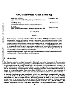
convergence monitoring should be avoided. The Markov nature of the Gibbs algorithm means that at convergence, the components of the simulated vector will generally be correlated to each other. Freulon [1992] showed on an experimental basis that i) the convergence towards the variogram is concomitant with the convergence towards the variance of the field to be simulated, and ii) when this latest condition is satisfied, the histogram is well reproduced. For this reason, the knowledge of the experimental variance of the field to be simulated allows one to easily control the number of iterations (it amount’s to comparing the experimental variance to the variance of the simulated field after each iteration). When the experimental variance is not known, one can use an empirical relationship between the average and the standard deviation of rainfields. One example of such a relationship is given in Figure 1 for the data set used below in section 4. The variance to reach as criterion of convergence of the algorithm is deduced from the areal value used for conditioning the simulation, based on the average relation shown in Figure 1.

4. Application to the unconditional simulation of Sahelian rain fields The purpose of this section is to verify whether in unconditional mode, the Gibbs sampling produces results comparable to those obtain by the TBM algorithm, which is classically used for the simulation of gaussian or gaussian-transformed random processes. To this end, data collected y the EPSAT-Niger monitoring network were used. This network covers a 16,000 km² area in the region of Niamey (Niger). A set of 456 independent rain fields has been simulated on an experimental grid of 400 regularly spaced points covering 10,000 km². The statistical properties of the simulated fields are compared in detail to those of the 456 events rain field observed from 1990 to 2000. In order to perform meaningful quantile-quantile comparisons, the simulated fields are re-sampled on 30 points with a geometry comparable to that of the long term EPSAT-Niger network.

Gibbs sampling for conditional spatial disaggregation of rain fields -13-

Version : 26/04/04

The Gibbs simulation procedure proposed here requires a preliminary estimation of i-) the pdf of y =( y i )i∈N and, ii-) the variogram or the covariance model to reproduce the spatial structure. Guillot [1999] showed that the points rain depth pdf can be represented by a mixture of gamma distribution and an atom at zero with descriptive parameters identical to those established for the ensemble of stations (see Table 1). Note that the meta-Gaussian model is fully described by the cdf of the point process (atom at zero, plus a pdf gamma distribution) and the covariance function. Furthermore, analysing the empirical covariances, Guillot [1999] observed two well-distinctive spatial structures characterized by an anisotropy axis directed E-N-E. Hence, the author propose to describe the spatial structure of the rain events through the following covariance model (C ) : − h1

C ( h) = σ e 2 1

s1

−h

+σ e 2 2

2

s2

(26)

where : h h i = h +  N  ai 2 E

  

2

(27)

where (hE , hN ) are the coordinates of h expressed on the base of the anisotropy axis ( hE along the E-N-E axis, along the N-W-N axis); ai is the anisotropy ratio of the structure i ; si is the scale distance parameter; and σ i2 is the scale variance parameter. The values used here are : σ 1 = σ 2 = 100 mm , a1 = 2 / 3 , a2 = 1 / 3 , s1 = 30 km and s2 = 300 km . 4.1. Observed parameters

The first step of the validation in unconditional mode is to assess the ability of the model to reproduce as well as possible the well known statistical properties derived from observations. A first analysis of the EPSAT-Niger data set was carried out by Guillot and Lebel [1999a] using 258 rain events over the period 1990-1995. The statistics of the 258-event

Gibbs sampling for conditional spatial disaggregation of rain fields -14-

Version : 26/04/04

data set are compared to those of the 456-event data set in Table 1, showing a remarkable stability of the statistical parameters between the two periods.

Table 1: Statistical parameters of the EPSAT-Niger events and related parameters of the corresponding Gamma distribution. The gamma distribution is fitted to the observed distribution of the conditional values of Y (Y>0). Period

Number of events

Mean:

Standard deviation:

Frequency of zero values:

m (mm)

σ (mm)

F0 (%)

1990-1995

258

10.8

14.2

26.0

1990-2000

456

10.9

14.4

25.4

Conditional values 1990-2000 (Y> 0) Parameters of the Gamma distribution

456

14.6

14.95

0

Scale parameter: 15.3 mm Shape parameter: 0.95 Atom at zero: 0.254

4.2. Parameters of the simulated fields

The values of the first three moments : proportion of zero values (F0 ) , mean (m ) and

( )

variance σ 2 are compared in Table 2. Concerning the mean and the variance, it is seen that there is a good agreement between the model outputs and the observations. The proportion of zero values is slightly underestimated by the proposed numerical approach: 23% according to the simulated rain fields against 25.4% for the observations. These results are comparable to those obtained with the TBM method – recomputed for the 1990-2000 sample – except for F0 which is better estimated by the TBM. Table 2: Comparison of the observed and simulated statistical parameters

Observations

Mean (mm) Variance (mm²)

F0 (%)

10.9

25.4

207.2

Gibbs sampling for conditional spatial disaggregation of rain fields -15-

Version : 26/04/04

Simulations Gibbs

10.6

201.3

23.0

Simulations TBM

10.9

199.1

25.4

4.3. Cumulative distribution functions of point rainfall

In this section, we will compare the distributions of the observed and simulated point rain depths. Figure 2 presents the quantile-quantile plot of the two distributions for the 456 events. For values smaller than 70 mm, there is a good agreement between the two distributions. Beyond this threshold, undulations in the scatter plot are observed. In order to test whether this behavior is linked to the sampling or whether it is predominantly linked to the model properties, each set of 456 events are divided into two sub-samples of 228 events. Figure 3.a presents the quantile-quantile plot of the fist 228 observed events versus the last 228 observed events. Figure 3.b presents the quantile-quantile plot of the first 228 simulated events versus the last 228 simulated events (first and last refered here to the order of appearance, not to the magnitude of the events). Obviously, these two plots are much less scattered than the observed versus simulated plot. This leads to the conclusion that it is the simulation algorithm rather than the sampling that causes the undulations observed in Figure 2. In term of spatial average rainfall distribution, one can observe in Figure 4 that the proposed model reproduces correctly the general behavior of the distribution. However, significant oscillations are observed on both sides of the one-one line. Finally, as seen in Figure 5, there is an overall good agreement between the observed and simulated fields in term of spatial standard deviation. 4.4. Spatial correlation structure

Gibbs sampling for conditional spatial disaggregation of rain fields -16-

Version : 26/04/04

To further evaluate the efficiency of the Gibbs algorithm, the spatial correlation structure of the simulated rain fields is also analyzed by comparing the average variogram of the 456 simulated events with the model used for the simulation (Figure 6). One can notice that the spatial correlation structure of the sahelian rain fields is very well reproduced by the model. 4.5. Fraction of area over threshold: unspecified property of the model

Several studies have shown the existence of a relation between the areal event rainfall and the fractional area where it rains above a given threshold [e.g. Doneaud et al., 1981; Kedem et Pavlopoulos, 1991]. An important step of the model validation is thus to assess its ability to reproduce this important property which was not specified in the model formulation. To this end, five classes of points value above a given threshold were constituted. The scatter plots – mean areal rainfall versus fraction area above threshold – of Figure 7 show a similar behavior in the observations and in the simulations (for the simulations a periodicity is observed in the sampling on the fraction of area axis, linked to the regular simulation grid used). The synthetic statistics given in Table 3 also show a good agreement between observations and simulations. The results of the Gibbs sampler are comparable to those obtained with the TBM by Guillot and Lebel (1999b). The results of Tables 2 and 3 constitute a global validation of the whole simulation model (representation of the rain field by a metaGaussian model, plus simulation of the meta-Gaussian process with the Gibbs sampler). This includes several approximations that had to be made for practical and theoretical reasons, most notably assuming the normality of ε in Equation 8 and using the variogram of Y as an approximation of the variogram of X in the kriging interpolation of the field of X. The good reconstitution of the areas over threshold, for a series of thresholds, is a more meaningful criterion than the simple reconstitution of the mean, variance, atom at zero and covariance function that are all used to build the model. Gibbs sampling in an unconditional mode

Gibbs sampling for conditional spatial disaggregation of rain fields -17-

Version : 26/04/04

performs similarly to the TBM in that respect, indicating that the convergence criterion used is adequate. Table 3 : Relation between the spatial average rainfall and the fractional area above a given thershold. The coefficient (r) reffers to the correlation between the spatial average rainfall and the fractional area where it rains above a thershold (see scatter plots in Figure 7). Class

Mean area above

Correlation coefficient (r)

threshold (%) Observations Simulations

Observations Simulations

h > 0 mm

77.21

74.82

0.71

0.69

h > 5 mm

48.64

52.12

0.87

0.83

h > 10 mm

35.98

35.87

0.92

0.91

h > 20 mm

19.77

17.01

0.95

0.97

h > 30 mm

10.05

8.33

0.93

0.94

5. Spatial disaggregation with the Gibbs sampler In the previous section, the ability of the Gibbs sampling to reproduce the statistical properties of the Sahelian event rain fields in an unconditional mode was evaluated. In the following, some indications are given on its efficiency in conditional disaggregation mode. To this end, the proposed numerical approach is applied to the conditional simulation of observed events over the study area. Its behavior is tested by comparing the statistical properties of the observed rainfield to those of 50 simulated rainfields sampled at the same space frequency. 5.1. Cumulative distribution functions

Gibbs sampling for conditional spatial disaggregation of rain fields -18-

Version : 26/04/04

As a preliminary step, the realism of the spatial disagregation algorithm in terms of cumulative distribution functions (cdf) is studied. The three examples presented here concern the spatial disagregation of the events recorded on the 12/07/1990 and on the 18/07/90 which can be considered as mean events in term of spatial average rain depth and the event recorded on the 08/08/1990 which is typical of a heavy rain event (Table 4). The events were chosen in 1990 because that year (as well as in 1991 and 1992) a larger number of recording raingauges was in operation, thus allowing to document each event with at least 50 stations. In Figure 8, the cumulative distribution curves of the first 10 conditional simulations for each of the three selected events are plotted. This figure shows a large internal variability of the model. This result clearly illustrates an intrinsic property of the spatial disagregation model which is its capacity to generate a large range of distributions for a given spatial average. One can also see in Figure 8 that the observed distribution is included in the envelop of the simulations. The comparison of the observed and the simulated cumulative distribution functions leads to the following two conclusions: i) despite the internal variability of the spatial disagregation model, there are several simulations with a cdf close to the cdf of the observations (in Figure 9, the closest of the 50 cdfs is compared to the observed cdf), ii) the extreme values are in general overestimated by the model.

Table 4 : Statistical parameters of three events observed over the study area Date

Mean (mm)

Standard deviation (mm)

F0 (%)

12/07/90

15.5

12.85

0.00

18/07/90

10.8

7.76

11.1

08/08/90

27.6

11.97

0.00

Gibbs sampling for conditional spatial disaggregation of rain fields -19-

Version : 26/04/04

In order to further validate the model in conditional mode the following procedure was carried out. For each of the three rainfields of table 4, the 29 observed rainfields with the closest average value to the average value of the event under consideration were selected (for instance for the 12/07/90 event the 29 events having their average value closest to 15.5 mm were extracted from the data base). Then the first 30 simulated fields (out of a total of 50) were resampled on a 50-point grid similar to the grid of observation, thus providing a set of 1500 (30*50) point values to be compared to the set of 1500 point observations. The corresponding quantile-quantile plots are shown in Figure 10, showing that they remain close to the one-one line. 5.2. Spatial organization of the simulated rain fields

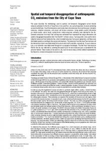
The 12/07/1990 event was chosen to illustrate the diversity of the spatial patterns that can correspond to a given areal rainfall. The observed spatial pattern is shown in Figure 11. The high values are located in the center of the study area. The first simulation shown in Figure 12 has an overall pattern very similar to that of the observations. This is only one example chosen in the series of 50 conditional simulations. On the other hand, since the spatial organization of event rain fields are characterized by a high degree of randomness, two events with equal spatial average and equal variance can display very different patterns. This is illustrated by the three others simulated fields shown in Figure 12 and demonstrates the skill of the model in producing a large range of spatial patterns associated to events of equal magnitude (spatial average) and equal dispersion (variance).

6. Conclusion A new method is proposed to perform conditional simulations of rainfields in the context of gaussian transformed functions. This method allows for the construction of various Gibbs sampling for conditional spatial disaggregation of rain fields -20-

Version : 26/04/04

scenarios of rainfields when only a spatially averaged estimate is known over a given area, whether this estimate comes from an atmospheric model or from a satellite sensor. The coupling of a Gibbs sampler to a so-called acceptation-rejection algorithm solves the limitation encountered when using turning band algorithms (TBM) which do not provide a consistent solution for simulation conditioned on known areal values. A comparison between TBM and Gibbs sampling in unconditional mode shows that the Gibbs sampler performs closely to the TBM, except for a slightly stronger unstability when looking at the distribution of point values. Spatial statistics are equally well reproduced by the Gibbs sampler and the TBM. From a theoretical point of view Gibbs and TBM should perform equally. Since the Gibbs sampling method presented here performs slightly worse than the TBM, there is likely room for improving the proposed algorithm, at least in unconditional mode. The real value of Gibbs sampling lies in its ability to carry out simulations conditioned on a known spatial value. Even though a complete validation of the model in conditional mode is not possible (it would require several dozen observed realizations with the same spatial average), it is possible to assess its realism by conditionally simulating several rainfields and comparing them to the observed rainfield and to other rainfields of similar magnitude. This comparison was carried out for three Sahelian rainfall events observed with the dense EPSAT-Niger network. For a given class of events, the conditional rainfields have a distribution of point values similar to the distribution of observed point values. At the same time the model is producing a wide range of spatial patterns corresponding to a single area average. This characteristic should allow to study a large spectrum of responses of the hydrological systems to the spatial pattern of rainfall in this region. Acknowledgements. Hubert Onibon gratefully acknowledged the Département Soutien

et Formation of IRD for a 3-year PhD funding. Abel Afouda also benefited from a funding Gibbs sampling for conditional spatial disaggregation of rain fields -21-

Version : 26/04/04

from DSF-IRD. The monitoring EPSAT-Niger network is operated in cooperation with Direction de la Météorologie Nationale of Niger. This research was carried out under a PNRH grant # 99-205.

References Allard, D., Connexité des ensembles aléatoires : application à la simulation de réservoirs pétroliers hétérogènes. Thèse de doctorat, Ecole Nationale Supérieure des Mines, Paris – France, 1993. Bardossy, A., and E. J. Plate, Space-time model of daily rainfall using atmospheric circulation patterns, Water Resour. Res., 28, 1247-1259, 1992. Doneaud, A., P.L. Smith, A.S. Dennis, and S. Sengupta, A simple method for estimating convective rain volume over an area, Water Resour. Res., 17, 1676-1682, 1981. Freulon, X., Conditionnement du modèle gaussien par des contraintes ou des randomisées, Thèse de doctorat, Ecole Nationale Supérieure des Mines, Paris – France, 1992. Galli, A., and H. Gao, Rate of convergence of the Gibbs sampler in the gaussian case, Mathematical Geol., 33(6), 653-677, 2001. Gelfand, A.E., and E.E.M. Smith, Sampling base approaches to calculating marginal densities, J. Am. Stat. Assoc., 85, 398-409, 1990. Geman, S., and D. Geman, Stochastic relaxation, Gibbs distribution and the bayesian restoration of images. IEEE Trans. Pattern Analysis and Machine Intelligence, 6, 721-741, 1984. Gleick, P. H., Regional hydrologic consequences of increases in atmospheric CO2 and other trace gases, Clim. Change, 10, 137-161, 1987. Grotch, S. L., and M. C. Mac Cracken, The use of general circulation models to predict regional climate change, J. Clim., 4, 286-303, 1991. Guillot, G., Approximation of Sahelian rainfall fields with meta-Gaussian random functions. Part 1: Model definition and methodology, Stoch. Env. Res. Risk Ass., 13, 100-112, 1999.

Gibbs sampling for conditional spatial disaggregation of rain fields -22-

Version : 26/04/04

Guillot, G., and Th. Lebel, Approximation of Sahelian rainfall fields with meta-Gaussian random functions. Part 2: Parameter estimation and comparison to data, Stoch. Env. Res. Risk Ass., 13, 113130, 1999a.

Guillot, G., and Th. Lebel, Disagregation of Sahelian meso-scale convective systems rains fields : further developments and validation, Journal of Geophysical Research, 104(D24), 31533-31551, 1999b. Harms and Campbell, An Extension to the Thomas-Fiering model for the sequential generation of streamflow, Water Resour. Res., 3(3), 653-661, 1967 Hostetler, S. W., Hydrologic and atmospheric models: The (continuing) problem of discordant scales, Clim. Change, 27, 345-350, 1994. Journel, A. G., and Ch. J. Huijbregts, Mining geostatistics, Academic Press, London New York San Francisco, 600p, 1978 Karl, T.R., W.C. Wang, M.E. Schlesinger, R.W. Knight, and D. Portman, A method of relating general circulation model simulated climate to the observed local climate, I, Seasonal statistics, J. Clim., 3, 1053-1079, 1990. Kedem, B., and H. Pavlopoulos, On the threshold method for rainfall estimation : choosing the optimal threshold level, J. Am. Stat. Assoc., 86(415), 626-633, 1991. Lantuéjoul, C., Non conditional simulation of stationary isotropic multigaussian random functions, in Geostatistical Simulations, edited by P.A. Dowd and M. Armstrong, pp 147-177, Kluwer Acad., Norwell, Mass, 1994. Lantuéjoul C., Iterative algorithms for conditional simulation, in Geostatistical Wollongong'96, vol. 1, edited by E. Y. Bafi and N. A. Schofield, pp 27-40, Dordrecht Kluwer, 1997. Le Barbé, L., T. Lebel, and D. Tapsoba, Rainfall variability in West Africa during the years 19501990, J. Clim., 15(2), 187-202, 2002. Lebel, Th., F. Delclaux, L. Le Barbé, and J. Polcher, From GCM scales to hydrological scales: Rainfall variability in West Africa, Stoch. Env. Res. Risk Ass., 14, 275-295, 2000.

Gibbs sampling for conditional spatial disaggregation of rain fields -23-

Version : 26/04/04

Matheron, G., The intrinsic random functions and their applications, Adv. Appl. Prob., 5, 211-222, 1973. Mejia, J.M., and J. Rousselle, Disaggregation models in hydrology revisited, Water Resour. Res., 12(2), 1856-186, 1976. Onibon, H., Simulation conditionnée des champs de pluie au Sahel : application de l'algorithme de Gibbs. Thèse de Doctorat, Institut National Polytechnique de Grenoble, Grenoble – France, 2001. Onof, C., N. G. Mackay, L. Oh, and H. S. Wheater, An improved rainfall disaggregation technique for GCMs, J. Geophys. Res., 103(D16), 19577-19586, 1998. Perrault, L., J. Bernier, B. Bobbée, and E. Parent, Bayesian change-point analysis in hydrometeorological time series. Part 1: The normal model revisited, J. Hydrol., 235, 221-241, 2000. Perica, S., and E. Foufoula-Georgiou, A model for multiscale disaggregation of spatial rainfall based on coupling meteorological and scaling descriptions, J. Geophys. Res., 101(D21), 26347-26361, 1996. Rind, D., C. Rosenzweig, and R. Goldberg, Modelling the hydrological cycle in assessments of climate change, Nature, 358, 119-122, 1992. Ritter, C., and M. A. Tanner, Facilitating the Gibbs sampler : the Gibbs stopper and the griddy Gibbs samplers, J. Am. Stat. Assoc., 87, 861-868, 1992. Roberts, G. O., Convergence diagnostic of the Gibbs sampler, In Bayesian statistics 4, edited by. J. M. Bernado, J. Berger, A. P. David, and A. F. M. Smith, pp 775-782, Oxford University Press, 1992. Sivapalan, M., and R.A. Woods, Evaluation of the effects of general circulation model’s subgrid variability and patchiness of rainfall and soil moisture on land surface water balance fluxes, in Scale Issues in Hydrological Modeling, edited by J.D. Kalma and M. Sivapalan, pp. 453-473, John Wiley, New York, 1995. Stedinger, J.R., D. Pei, and T.A.Cohn, A condensed disaggregation model for incorporating parameter uncertainty into monthly reservoir simulations, Water Resour. Res., 21(5), 665-675, 1985.

Gibbs sampling for conditional spatial disaggregation of rain fields -24-

Version : 26/04/04

Von Neuman, J., Various techniques used in connection with random digits, National bureau of standards Appl. Math. Ser., 2, 36-38, 1951. Wigley, T. M. L., P. D. Jones, K. R. Briffa, and G. Smith, Obtaining sub-grid scale information from coarse resolution general circulation model output, J. Geophys. Res., 95, 1943-1953, 1990. Wilby, R.-L., A comparison of downscaled and raw GCM output: implications for climate change scenarios in the San Juan River basin, Colorado, J. Hydrol., 225, 67-91, 1999. Wilks, D.-S., Conditioning stochastic daily precipitation models on total monthly precipitation, Water Resour. Res., 25, 1429-1439, 1989. Wilson, L.-L., D.-P. Lettenmaier, and E. F. Wood, Simulation of precipitation in the Pacific Northwest using a weather classification scheme, Survey Geophys., 12, 127-142, 1991.

Gibbs sampling for conditional spatial disaggregation of rain fields -25-

Version : 26/04/04

List of Figures Figure 1. Relationship between the areal rain depth and the standard deviation of point values for the 456 events of the EPSAT-Niger data set. Figure 2. Quantile-quantile plot of the observed and simulated point rainfall (456 observed events and 456 simulated events resampled on a set of 30 points with a configuration close to that of the observation network). Figure 3. Quantile-quantile plot of the first and last 228 rain depths: a. observations; b. simulations. Figure 4. Quantile-quantile plot of the observed and simulated spatial average rainfall (456 events). Figure 5. Quantile-quantile plot of the observed and simulated spatial standard deviation (456 events). Figure 6. Comparison of the theoretical variogram with the mean variogram of the simulated events. Figure 7. The relation between the fractional area where it rains above a given threshold and the mean areal rainfall. Comparison between observations (left) and simulations (right). Figure 8 : Cumulative distribution functions of the first ten conditional simulations (resampling on 50 points) compared to that of the observations (50 points). Figure 9 : Cumulative distribution function of the observations compared with the cumulative distribution function of one particular simulation. Figure 10. Quantile-quantile plot of point values from 30 simulations and 30 observed rainfields. The 30 observed rainfields were chose based on their average value being as close as possible of the average value of the event used for conditioning the simulations (see Table 4). The observed fields and simulations are sampled at 50 points. The total number of points in each plot is thus equal to 1500. Figure 11. Spatial distribution of the cumulatd values observed during the event of 12/07/90 Figure 12. Examples of the conditional simulations obtained for the event of 12/07/90

Gibbs sampling for conditional spatial disaggregation of rain fields -26-

Version : 26/04/04