RANDOLPH E. BANKy AND DONALD J. ROSEz. Abstract. We derive a class of globally .... de ned as follows: Ak gk + g0 kxk jjgkjj ;. (2.6) k. jjAkjj; and. Bk. R1.
GLOBAL APPROXIMATE NEWTON METHODS � RANDOLPH E. BANKy AND DONALD J. ROSEz
Abstract. We derive a class of globally convergent and quadratically converging algorithms for a system of nonlinear equations g(u) = 0, where g is a su�ciently smooth homeomorphism. Particular attention is directed to key parameters which control the iteration. Several examples are given that have successful in solving the coupled nonlinear PDEs which arise in semiconductor device modelling. AMS subject classi cations. 65H10
1. Introduction. In this paper we derive an algorithm for solving the nonlinear
system (1.1)
g(u) = 0
where g = (g1 ; g2 ; : : : ; gn )T is a su�ciently smooth homeomorphism from IRn to IRn . Recall that a homeomorphism is a bijection (1-1, onto) with both g and the inverse map, g?1 , continuous. Physically, a homeomorphism means that the process modelled by g has a unique solution x for any set of input conditions y, i.e., g(x) = y, and that the solution x varies continuously with input y. Sometimes this notion is referred to as a \well-posed" process g. Actually, the requirement that g be a homeomorphism is a special case of our assumptions, but we defer a more detailed and general discussion to Section 2. In its generic form the algorithm we propose is well known. Starting at some initial guess u0, we solve and n � n linear system (1.2)
Mk xk = ?g(uk ) � ?gk
and then set (1.3)
uk+1 = uk + tk xk :
We call the method an approximate Newton method because Mk will be chosen to be related to the Jacobian g0 (uk ) � gk0 , in such a manner that xk approximates the Newton step wk = ?fg(uk )0 g?1g(uk ), and because usually tk 6= 1. In many applications, (1.2) can be interpreted as an \inner" iterative method for solving the linear system (1.4)
gk0 wk = ?gk :
When g is a smooth homeomorphism, we will show how to choose the damping parameters tk and the approximate Newton steps xk such that the uk converge to u� with g(u�) = 0 quadratically for any initial u0 (see Section 2 for the notions of quadratic and more general higher order convergence). The choice of xk = wk in (1.4), the damped Newton method, in an important special case. In Section 2 we show that, for any choice of norm j �jj, the choice tk = (1+Kjjgk j )?1 for some sequence 0 � Kk � K0 produces the convergence mentioned above. More � Received by the editors September 17, 1980. y Department of Mathematics, University of California z Bell Laboratories, Murray Hill, New Jersey 07974.
1
at San Diego, La Jolla, California 92093.
precisely, for K0 su�ciently large, the sequence j gk j decreases monotonically and quadratically to zero. While it is possible in theory to take Kk = K0 for all k, such a strategy often leads to the quagmire of slow initial convergence and can prove disastrous in practice (see Sections 3-4). As we shall see, this rule for choosing tk is motivated by the requirement tk ! 1 such that 1 ? tk = O(j gk j ). By specifying a formula for picking tk , we attempt to avoid most of the searching common to other damping strategies. We also show in Section 2 how to choose the xk (or Mk ) in (1.2) such that the xk approximates wk of (1.4). In this setting our analysis continues and extends investigations of approximate Newton methods initiated by Dennis and Mor�e (see [5, 6]). Motivated by problems in optimization where it may be di�cult or undesirable to deal with the Jacobian, gk0 , they choose Mk , for example, such that (1.5) j fMk ? g(u�)g(uk+1 ? uk )j j uk+1 ? uk j ?1 ! 0 to obtain superlinear convergence. Equation (1.5) may not be immediately useful in contexts where Mk represents an iterative process for solving (1.4); contexts, for example, arising from nonlinear PDEs where it is often possible to evaluate gk0 but it may not be easy to solve (1.4) exactly. Sherman [12] discusses such Newton-iterative methods, showing that to obtain quadratic convergence it su�ces to take mk = O(2k ) inner iterations as k ! 1. Computationally, it is more convenient to measure the extent to which xk approximates wk by monitoring the quantity j gk0 xk + gk j , that is, checking the residual of (1.4) when xk replaces wk . To obtain quadratic convergence, for example, we choose xk such that 0 (1.6) � � j gk xk + gk j � cj g j ; k
j gk j
k
c > 0, with xk 6= 0, a suggestion also made by Dembo, Eisenstat and Steihaug [4].
The discussions by the above named researchers all deal with local convergence; that is, they examine convergence in a local region containing a root u� such that the choice tk = 1 is appropriate. We derive (1.6) within a global framework consistent with our choice of tk ; that is we require �k = O(j gk j ) to balance the quantity 1 ? tk = O(j gk j ). We also show that conditions such as (1.6) are equivalent to the original conditions imposed by Dennis and Mor�e. The whole key to our analysis is the judicious use of the Taylor expansion: (1.7) gk+1 = gk + gk0 fuk+1 ? uk g +
Z1
0
fg0 (uk + s(uk+1 ? uk )) ? gk0 gfuk+1 ? uk g ds
or, using (1.3) and the notation of Section 2 (1.8) gk+1 = (1 ? tk )gk + tk j gk j (gk0 xx + gk )j gk j ?1 +
Z1
0
G(s; uk+1 ; uk )tk xk ds:
Taking norms will lead to (1.9) j gk+1 j � j gk j f(1 ? tk ) + tk �k + t2k k j gk j g 2
under appropriate conditions on the smoothness of g and the sequence Mk?1 . Since k will be bounded, (1.9) shows it is possible to insure that the j gk j ! 0 monotonically and quadratically by forcing each term in braces to be O(j gk j ). Finally, note that (1.7) can be interpreted in a Banach space, and the extension of our results to such a setting is immediate (see [13], Section 12.1). Section 2 contains a detailed discussion of our assumptions and global convergence analysis. Section 3 encodes the analysis of Section 2 into a general algorithm. Section 4 presents a further algorithmic discussion and discusses several important examples. We conclude in Section 5 with some numerical results relevant to the solution of semiconductor device partial di�erential equations. The authors acknowledge discussions with S. Eisenstat, I. Sandberg (see [10, 11]), and W. Fichtner and appreciate the support and encouragement of J. McKenna. 2. Parameter Selection and Convergence. Given an arbitrary initial iteration u0 , we consider here the convergence of the iteration (1.2)-(1.3) where the parameters tk are chosen by the rule tk = 1 + K1 j g j : (2.1) k k We make the following assumptions on the mapping g(u) and the sequence Mk . Assumption A1: The closed level set (2.2)
S0 = fuj j g(u)j � j g0 j g
is bounded.
Assumption A2: g is di�erentiable?and the Jacobian g0 (u) is a continuous and 1 nonsingular on S0 , and the sequence j Mk j is uniformly bounded, i.e., (2.3) j Mk?1 j � k1 on S0 for all k � 0: We embed S0 in the closed convex ball (2.4)
�
�
S1 = uj j uj � sup j vj + k1 j g0 j : v2S0
Assumption A3: The Jacobian g0 is Lipshitz; i.e., (2.5) j g0 (u) ? g0 (v)j � k2 j u ? vj ; u; v 2 S1 : Without loss suppose gk = 6 0 for all k, and let the quantities Ak , �k , Bk , k be
de ned as follows: (2.6) and (2.7)
0
Ak � gk +j g gjk xk ; k �k � j A k j ; R1 0 0 Bk � 0 fg (uk +(stt kjxgk )j )?2 gk gtk xk ds k k k � j Bk j ; 3
for tk , uk , and xk as in (1.2)-(1.3). The parameters �k measure the extent to which the xk of (1.2) di�er from the Newton correction (�k � 0). For uk 2 S0 note that
�k � k1 j gk0 ? Mk j : Typically, given the sequence j gk j and �0 2 (0; 1), we will consider the convergence process when all �k � �0 and (2.9) �k � cj gk j p for p 2 (0; 1], c > 0: (2.8)
for example,
�
� �p �p j g j j g j k k �k � �0 j g j = �k?1 j g j : 0 k?1
(2.10)
For many Newton-like methods the �k can be easily computed, and �0 and p can be speci ed a priori. The parameters k re ect the size of higher (second) order terms which are ignored in the derivation of a Newton-like method. For uk+1 = uk + tk xk 2 S1 and uk 2 S0 , (1.2), (2.3), (2.5), and (2.7) imply
� �2 2 k j x j 2 k k � 2 j g j � k12k2 (2.11) k Suppose uk+1 2 S1 and uk 2 S0 . Taylor's Theorem ([9], Section 3.2) implies
gk+1 = gk + g0 fuk+1 ? uk g + k
(2.12)
Z1
fg0(uk + s(uk+1 ? uk )) ? gk0 g(uk+1 ? uk ) ds = (1 ? tk )gk + Ak tk j gk j + Bk t2k j gk j 2 ; 0
Ak and Bk as above. Equation (2.12) immediately yields the Taylor inequality � (2.13) j gk+1 j � j gk j (1 ? tk ) + �k tk + k t2k j gk j : We will show the sequence j gk j ! 0 by analyzing the term in braces. Proposition 2.1. Let � 2 (0; 1 ? �0), �0 2 (0; 1) and tk chosen as in (2.1) where (2.14) 0 � K k � K0 and
(2.15)
2
Kk � 2(1 ?k1�k2 ? �) ? j g1 j : k
k
Assume A1-A3 and all �k � �0 . Then (i) all uk 2 S0 , the sequence j gk j is strictly decreasing and j gk j ! 0; furthermore, (ii) j gk+1 j =j gk j ! 0 if and only if �k ! 0, and for any xed p 2 (0; 1],
(2.16)
j gk+1 j � c1 j gk j 1+p
if and only if
(2.17)
�k � c2 j gk j p 4
for positive constants c1 and c2 . Proof. To show (i), suppose uj 2 S0 and j gj j < j gj?1 j for 1 � j � k. Since uk+1 = uk + tk Mk?1gk , j uk+1 j � j uk j + k1 j gk j so uk+1 2 S1 . Thus (2.11) and (2.15) imply Kk � 1 ? � k ? � ? j g1 j (2.18) k k
Rearranging (2.18) and using (2.1) shows (2.19)
(1 ? tk ) + �k tk + k t2k j gk j � 1 ? �tk ;
hence (2.20)
j gk+1 j � (1 ? �tk )j gk j � (1 ? �t0 )j gk j
recalling (2.13). Equation (2.20) implies the conclusion (i). Part (ii) follows from the pair of inequalities
j gk+1 j � (K + k2 k =2)j g j + � k k k 1 2 j gk j
(2.21) and (2.22)
�k � (1 + Kk j gk j ) j gj kg+1j j + (Kk + k12 k2 =2)j gk j k
since j gk j ! 0. Recalling tk � 1, Equations (2.21)-(2.22) are immediate from (2.13) and the analogous inequality derived by transposing (2.12). Note that (2.15) is satis ed for the constant sequence
Kk = K0 for all k: Furthermore (2.15) allows the choice Kk = 0 when (2.24) j g j � 2(1 ? �k ? �) :
(2.23)
k
k12 k2
However, as noted in Section 1, (2.23) can be quite unsatisfactory, and we have chosen to force tk ! 1 by using (2.1) rather than using a test to determine whether the choice tk = 1 is satisfactory as eventually guaranteed by (2.24); see Sections 3-4. We will show later that the sequence uk converges to the root u� with g(u�) = 0. Recall that convergence is superlinear if
j uk+1 ? u�j � �k j uk ? u� j and �k ! 0; it is order Q ? (p + 1), (p 2 (0; 1]) if (2.26) j uk+1 ? u� j � cp j uk ? u� j p+1 cp > 0:
(2.25)
Convergence is R-linear if (2.27)
j uk+1 ? u� j � �k+1 5
and if
�k+1 � c�k ;
c 2 (0; 1): To examine the nature of the convergence of fuk g we consider the relationship between j gk j ! 0 and j uk ? u� j ! 0. Consider the Taylor expansion
(2.28)
0 = g(u� ) = gk + g0 fu� ? uk g + k
Z1
0
(2.29) = gk + gk0 tk xk + gk0 fu� ? uk+1 g +
fg0(uk + s(u� ? uk )) ? gk0 gfu� ? uk g ds Z1
0
fg0 (uk + s(u� ? uk )) ? gk0 gfu� ? uk g ds
Sine g0 is continuous and invertible on S0 , j (gk0 )?1 j � k3 ; rearranging the second inequality of (2.29) implies
j uk+1 ? u� j � k3 f(1 ? tk )j gk j + tk �k j gk j + (k2 =2)j uk ? u� j 2 g: Letting k5 = supu2S1 j g0 (u)j , note (2.31) j gk j � k5 j uk ? u� j ; (2.30)
hence,
j uk+1 ? u� j � j uk ? u�j k3 fk5 �k + (k52 K0 + k2 =2)j uk ? u�j g using (2.1) and tk � 1. Equation (2.32) shows that the convergence of fuk g to u� is superliner if �k ! 0 and is of order Q ? (p + 1) if �k � c2 j gk j p , again using (2.31). Suppose that in some set S � S0 (2.31) can be extended to (2.33) k4 j uk ? u�j � j gk j � k5 j uk ? u�j : (2.32)
Then under the conditions of Proposition 2.1, it is immediate from (2.20),, (2.21), and (2.33) that the convergence of fuk g tp u� is: (i) R-linear, and furthermore (ii) superlinear if and only if j gk+1 j =j gk j ! 0, and; (iii) order Q ? (p + 1) if and only if j gk+1 j � c1 j gk j p+1 , p 2 (0; 1]. In general (2.33) may not be valid on the entire set S0 . However (2.29) implies (2.33) for uk su�ciently close to u� as follows. The rst inequality in (2.29) leads to (2.34)
j uk ? u�j f1 ? (k2 k3 =2)j uk ? u�j g � k3 j gk j :
Thus for any � 2 (0; 1) (say � = 1=2), (2.34) and (2.31) imply (2.33) for S = S0 \ S� where � � 2(1 ? � ) � S = uj j u ? u j � (2.35) �
k2 k3
and k4 of (2.33) is k4 = �k3?1. Summarizing Proposition2.1 and the discussion involving (2.25)-(2.35) we have Theorem 2.2. Under the conditions of Proposition 2.1 (i) there exists a u� 2 S0 with u� = lim uk and g(u�) = 0; (ii) on S0 the convergence of fuk g to u� is superlinear or order O ? (p + 1) if �k ! 0 or �k � c2 j gk j p , respectively; 6
(iii) on any set S = S0 \ S� as in (2.35), the convergence of fuk g to u� is at least R-linear; it is superlinear or order Q ? (p + 1) if and only if �k ! 0 or �k � c2 j gk j p , respectively. Proof. It remains only to show (i), which we establish by showing that fuk g is a Cauchy sequence. But since
(2.36)
k+j ?1 X X j uk+j ? uk j = ti xi � k1 j gi j ; i i=k
and the j gk j ! 0 with j gk+1 j � cj gk j , c < 1, fuk g is clearly Cauchy with a limit u� in the closed set S0 . Continuity of g implies that g(u� ) = lim g(uk ) = 0. We now have the following global result. Theorem 2.3. Let G : IRn ! IRn be a homeomorphism. Suppose g0 is Lipschitz on closed bounded sets and A2 is satis ed. Then, given any u0 , the sequence uk of (1.2)-(1.3) with tk as in (2.1) and Kk as in (2.15) converges to u� as in Theorem 2.2. Proof. Since g0 is Lipschitz on closed bounded sets, g0 is continuous on IRn . Thus j g(u)j ! 1 as j uj ! 1 since g is a homeomorphism ([9], page 137). Hence S0 of (2.2) is bounded for any u0 and A1 and A3 are satis ed. The result now follows from Theorem 2.2. As mentioned in Section 1, early investigations by Dennis and Mor�e examined higher order convergence of approximate Newton methods. In our notation, they characterized convergence by studying the quantity j (Mk ? g0 (u� ))xk j =j xk j where they chose xk = uk+1 ? uk (tk = 1). Their results can be recast in the framework of Theorem 2.2 as the following Theorem 2.4. (cf. [6], pages 51-52). In addition to the conditions of Proposition2.1, let j Mk j � k6 . Then (i) on any set S = S0 \ S� , S� as in (2.35), convergence of fuk g to u� is superlinear if and only if j (Mk ? g0 (u� ))xk j ! 0 (2.37)
j xk j
while on S0 , (2.37) implies superlinear convergence; (ii) on S convergence is Q ? (p + 1) if and only if
(2.38)
j (Mk ? g0 (u� ))xk j � � j x j p ; p 2 (0; 1]: p k j xk j
Proof. The conclusion follows from the pair of inequalities 0 � � � k j (Mk ? g (u ))xk j + k k j u ? u� j ; (2.39) k
and (2.40)
1
1 2 k
j xk j
j (Mk ? g0 (u� ))xk j � � j gk j + k2 j g j ; k jx j k k j xk j k 4
which can be derived from the de nitions of �k and the constants ki . For example, to show the \only if" part of (ii), we rst note that Q ? (p + 1) convergence implies 7
(Theorem 2.2) that �k � c2 j gk j p � c2 k6p j xk j p . Hence by (2.40) j (Mk ? g0 (u� ))xk j � c kp+1 j x j p + k2 k6 j x j 2 6 k jx j k k k
� � p j xk j p :
4
The other conclusions follow similarly. We conclude this section with some remarks concerning the generality of the analysis presented here. Remark R1: If Holder continuity, i.e., (2.41) j g0 (u) ? g0 (v)j � ke j u ? vj e ; v; u 2 S1 ; e 2 (0; 1) replaces Lipschitz continuity in A3, the above analysis remains valid with minor modi cations including the restriction of the order exponent p to p 2 (0; e]. In fact, if g0 is only uniformly continuous on S1 (continuous in IRn ), then (2.42) j g0 (u) ? g0(v)j � w(j u ? vj ) where w(t) is the modulus of continuity for g0 on S1 (see [9], page 64). Again much of the analysis remains valid; however, it is now only possible to obtain superlinear convergence. The restriction on Kk analogous to (2.15) in this case is � � (2.43) w 1 +k1Kj gkj jg j � 1 ? �k k ? � ; k k 1 showing it is possible to choose 0 � Kk � K0 since w is an isotone continuous function with w(0) = 0. See Daniel ([3], Section 4.2, Chapter 8) and Sanberg [11] for discussions of the role of uniform continuity in similar contexts. Remark R2: Note that (1.2) and (1.3) can be replaced by any procedure for determining xk such that (2.44) 0 < j xk j � k1 j gk j : In all our applications, however, xk can be shown to derive from gk by a linear relationship of the form (1.2). Furthermore, the bound on j Mk?1 j usually follows from the continuity and invertibility of g0 on S0 in addition to convergence assumptions on the inner process which determines xk (see Section 4). In the spirit of R1, it is also possible to generalize (2.44) to (2.45) 0 < j xk j � k1 j gk j s ; s 2 (1=2; 1] for g0 Lipschitz on S1 . If g0 is less smooth, s must be suitably restricted. Remark R3: As we have seen in Theorems 2.2 and 2.4, the inability to extend (2.33), in general, to the entire set S0 leads to somewhat disquieting technicalities concerning the necessary conditions on the convergence to zero of the sequence f�k g. In the important special case that g(u) is uniformly monotine on S0 , i.e., (2.46) (g(u) ? g(v))T (u ? v) � k7 (u ? v)T (u ? v); the Cauchy-Schwarz inequality implies (in the 2-norm) that (2.47) k7 j u ? u� j 2 � j g(u)j 2 on S0 . Hence (2.33) is valid on S0 and the appropriate statements in Theorems 2.2 and 2.4 can be simpli ed. In an algorithmic setting, however, note that statements (i) and (ii) of Theorem 2.2 are the real content of the result. 8
3. Algorithm. We now turn to the computational aspects of the analysis described in Section 2. In particular, we consider the problem of determining the Kk of (2.1) such that (2.15), or more importantly (2.18), is satis ed. Note that inequality (2.20) can be rewritten as (3.1)
�
� j g j k +1 � � 1 ? j g j t1 : k k
Since the right-hand side of (3.1) is easily computed, and since we may choose � 2 (0; 1 ? �0 ), equation (3.1) is a convenient test. Failure to satisfy (3.1) implies Kk fails to satisfy (2.18). We then increase Kk and compute new values for tk and gk . These increases will eventually lead to Kk satisfying (2.15), (2.18), and (3.1), and this process leads to convergence as in Proposition 2.1. Consider the choice of K0 . Given a guess, say K0 = 0, each failure of the test (3.1) requires a function evaluation of g(u) to compute a new g1 . This aspect of the procedure has the avor of a line search, but with one important di�erence. Once a value of K0 has been accepted, one might reasonable expect to pass (3.1) for Kk = K0 on almost all subsequent iterations k. However, note that as j gk j decreases, the righthand side of (2.18) decreases, suggesting the possibility of taking Kk � Kk?1 . If the Kk decrease in a orderly manner (for example Kk = Kk?1 =10), we anticipate a process which uses only one function evaluation on most steps. In fact decreasing the Kk can be important; we have found than an excessively large value of K0 will cause the convergence of tk ! 1 to be much slower than necessary, delaying the onset of the observed superlinear convergence, and possibly resulting in many iterations. The above discussion motivates the following algorithm.
Algorithm Global (1) input u0 , � 2 (0; 1 ? �0 ) (2) K 0, k 0; compute g0 , j g0 j (3) compute xk (4) tk (1 + Kjjgk j )?1 (5) compute uk+1 , gk+1 , j gk+1 j (6) if (1 ? j gk+1 j =j gk j )t?k 1 < � (7) then fif K = 0, then K 1; else K 10Kg; GOTO (4) (8) else fK K=10; k k + 1g (9) if converge, then return; else GOTO (3)
In Global, failure to satisfy (3.1) causes K to be increased in line (7). Each failure requires on additional function evaluation on line (5). On line (8), we take K=10 as the initial estimate for Kk+1 . Alternatively, we have considered Kk+1 = Kk 4j?k?1 where j is the last index resulting in a failure of the test on line (6). In practice, we have found these methods for decreasing K to be a reasonable compromise between the (possibly) con icting goals of having tk ! 1 quickly and having (3.1) satis ed on the rst function evaluation for most steps. The procedure for increasing K is also important, and we have found a procedure other than the relatively simple one given on line (7) to be advantageous. In this scheme, one speci es a priori the maximum number of function evaluations to be allowed on a given step, say ` (typically ` = 10), The trial values of K denoted Kk;j , 9
1 � j � `, satisfy �
k?1 (3.2) Kk;j = j g1 j + K10 k
��
j xk j �((j?1)=(`?1)) ? 1 ; for j xk j > �: �j uk j j gk j j uk j 2
This corresponds to the easily implemented formulae (3.3)
tk;1 = (1 + Kjjgk j =10)?1 ; tk;j = tk;1 (�j uk j j xk j )((j?1)=(`?1))2 ;
2 � j � `:
We take � to be a constant on the order of the machine epsilon �103. For small values of j � 2, tk;j represents a modest decrease of tk;j?1 . As j increases, tk;j decreases more rapidly until tk;` j xk j = j uk j �tk;1 . If (3.1) fails for tk;` , the calculation is terminated and an error ag set. Equations (3.3) represent a compromise between the con icting goals of increasing K slowly (so as not to accept a value which is excessively large) and of nding an acceptable value in few function evaluations. On line (3) we have not detailed the computation involving (1.2). If Mk = gk0 in (1.2), Global is a damped Newton method and �k = 0 for all k (disregarding round o�). Alternatively, (1.2) may represent an iterative process for solving gk0 xk + gk = 0 terminated when �k satis es some tolerance such as (2.9)-(2.10). Such damped Newton methods and other approximate Newton methods are outlined in the following section. 4. Applications. In this section we present several applications for the results in the previous sections. In particular, we show how Newton-iterative methods, Newtonapproximate Jacobian methods, and other Newton-like methods t within our global approximate Newton framework. 4.1. Newton-Iterative Methods. Suppose that xk in line (3) of algorithm Global is computed by using an iterative method to solve the Newton equations
gk0 wk = ?gk :
(4.1)
For example, we might use a standard iterative method such as SOR or a NewtonRichardson method where gk0 in (4.1) is replaced by a previous Jacobian gk0 . The Newton-Richardson choice is useful when a (possibly sparse) LU factorization of the Jacobian is relatively expensive. Hence the Jacobian is factored infrequently, and in outer iterations where the factorization is not computed, we iterate to approximately solve (4.1) using the last computed factorization. (see [12]). In all such Newton-iterative methods ([9], Section 7.4), we suppose gk0 has a uniformly convergent splitting on S0 ; i.e., 0
gk0 = Ak ? Bk
(4.2) with j Hk j � �0 < 1 for all k, where (4.3)
Hk = Ak?1 Bk = I ? A?k 1 gk0 :
We then compute xk by computing the inner iteration (4.4)
Ak xk;m = Bk xk;m?1 ? gk 10
until m = mk , taking xk;0 = 0 and setting xk = xk;mk . Note that (4.4) can be rewritten as
Ak (xk;m ? xk;m?1 ) = ?(gk0 xk;m?1 + gk ): Using induction and (4.3), it can be shown that the xk;m in (4.4) satisfy (4.6) gk0 (I ? Hkm )?1 xk;m = ?gk ; m � 1: Hence we may identify Mk of (1.2) with Mk = gk0 (I ? Hkmk )?1 , and these Mk satisfy (2.3) since j (gk0 )?1 j is bounded on S0 and j I ? Hkmk j � 2. (4.5)
Notice that the right hand side of (4.5) contains the Newton residual which suggest de ning the quantities 0 � � j gk + gk xk;m j (4.7) k;m
j gk j
in analogy with (2.6) and the quantities xk;m . The �k;m are easily computed, certainly when the iteration proceeds as in (4.5) rather then (4.4). Since we have assumed that the Ak and Bk are a convergent splitting, �k;m ! 0 as m ! 1. Thus to obtain convergence as discussed in Section 2, we stop the inner iteration when �k;m attains the desired tolerance �k � �k;mk . For example, to obtain orer Q ? (p + 1) superlinear convergence, p 2 (0; 1], we stop after mk iterations where (4.8)
�p � �k;m � �0 jj ggk jj ; 0
�0 2 (0; 1);
as in (2.9)-(2.10). Note that (4.9)
0 xk;m = H^ m gk gk + gk;m k
where Hk = gk0 H^ k (gk0 )?1 ; this implies (4.10)
�k;m � j H^ k j m
Assuming (4.1) is an equality with j H^ k j < 1 and that equation (2.16)-(2.17) are equalities, we see that p mk = log c2 j^gk j : (4.11) log j Hk j Asymptotically (as k ! 1) we expect j H^ k+1 j � j H^ k j ; again assuming equality and using (2.16)-(2.17) and (4.11) shows (4.12)
mk+1 � (1 + p)mk :
Hence for k su�ciently large we can expect the number of inner iterations per outer iteration to approximately increase by a factor of (1 + p). In the preceding general analysis of Newton-iterative methods all �k = �k;m are possibly nonzero. For the special case of a Newton-Richardson method a decision is made at the beginning of the k-th outer iteration whether to factor gk0 thus doing an \exact" damped Newton iteration. Such a factorization implies �k = 0; otherwise the 11
inner iteration corresponds to a splitting with Ak = gk0 , k0 < k, where Ak has been previously factored. It is not di�cult to decide when to refactor: one should refactor when the total cost of inner iterations using the factored gk0 just surpasses the cost of a new factorization. For example, using nested dissection on an n � n mesh cost approximately 10n3 operations for a factorization and 5n2 log2 n operations for a backsolution. Thus approximately 2n= log2 n inner iterations compared with a new factorization. Note however that initially these 2n= log2 n inner iterations will be part of several outer iterations monitored by the �k;m ; each time a new such outer iteration is started, gk0 is computed (but not factored) for use in the right hand side of (4.5). The relative time T1 corresponding to 10n3 and T2 corresponding to 5n2 log2 n can often be timed dynamically using a \clock routine" and need not be known a priori. As a nal remark, note that superlinear convergence will require an increasing number of inner iterations, and ultimately, the inner iteration time will surpass the cost of a new factorization. However, in practice when only a modest overall accuracy is required Newton-Richardson methods can prove to be highly e�ective, and we have found such cases. 4.2. Newton-Approximate Jacobian Methods. When the partial derivatives required for the computation of gk0 are unavailable or expensive to compute, it is common to approximate gk0 , perhaps using nite di�erences ([6], page 49, [9], pages 185-186). We denote such an approximation to gk0 by g~k0 . We assume that the g~k0 satisfy 0
0
j gk0 ? g~k0 j � k�k
(4.13)
1
for �k < 1. Let Ak of (2.6) be written as
Ak = A~k + �k
(4.14) where (4.15)
0
0
0
g~k )xk �k = (gk ? jg j :
A~k = gk +j g g~jk xk ; k
k
Following (2.6), let �~k = j A~k j and note that j �k j � �k ; hence
�k � �~k + �k :
(4.16)
If xk is obtained by the linear system
g~k0 xk = ?gk ;
(4.17)
then �~k = 0, corresponding to Mk = g~k0 in (1.2). Alternatively (4.17) can be solved approximately, perhaps by a Newton-iterative method as in Section 4.1; then �~k 6= 0 in general. If all �~k = 0 the �k play the role of �k in Section2. For example, if all �~k = 0 and (4.18)
�p j g j k �k � �0 j g j ; p 2 (0; 1]; �0 < 1; 0 �
12
then the Newton-approximate Jacobian scheme will converge with order Q ? (p + 1). More generally, let �~k 6= 0 and �k satisfy (4.18) with (4.19)
�
�
�q � j g j k �~k � max �~0 j g j ; �k ; �~0 + �0 < 1: o
In a typical situation we might have p = 0, q = 1, and �0 small; i.e., we compute the approximation to gk0 to a xed accuracy and use an iterative method to solve (4.17) approximately. For the rst few outer iterations, relatively few inner iterations will be required. The inner iterations will increase until �k becomes the larger of the two terms on the right-hand side of (4.19). From this point onward, approximately a constant number of inner iterations will be used, and the asymptotic outer convergence will be R-linear (Theorem 2.2). It may not be easy to estimate or compute �k ; although, if we are computing g~k0 to a xed accuracy, we expect all �k to be approximately equal. Since �k enters the computation only through (4.19), we see that its main purpose is to prevent useless inner iterations. If nothing is known about �k , we can set all �k = � in (4.19), � a su�ciently small number. Convergence of the outer iteration can loosely be described as superlinear at the beginning and ultimately linear depending on the actual values of �k . The choice of � could have a signi cant e�ect on the total computation cost and may require some experimentation. 4.3. Two Parameter Damping. In an earlier investigation, [1], we studied the Newton-like method (4.20) (4.21)
(I=sk + gk0 )xk = ?gk ; uk+1 = uk + xk ;
motivating the method by considering Euler integration on the autonomous system of ODEs (4.22)
du + g(u) = 0; dt
u(0) = u0 :
Under appropriate conditions, including the uniform monotonicity of g(u) on IRn in the form (4.23)
xT g0 (u)x � k7 xT x;
we showed that it is possible to obtain global quadratic convergence by forcing sk j gk j to be a su�ciently small constant for all k. We used a norm reducing argument similar to the analysis of Section 2. Here we sketch a more general treatment using the results of Section 2. Consider the iteration (1.2)-(1.3) with tk as in (2.1), �k � 0, and (4.24)
Mk = �k j gk j I + gk0 :
We call such a method two parameter damping because the �k as well as the tk limit the change (uk+1 ? uk ). It is immediate from (4.24) that the �k of (2.6) satisfy
�k = �k j xj k : If the j Mk j are uniformly bounded (for all �k ) as in (2.3), then (4.26) �k � k 1 �k j g j k : (4.25)
13
This shows that the �k can be chosen such that �0 < 1 and �k � �0 as in Proposition 2.1. Furthermore, the Q-quadratic convergence (2.16) is also a consequence of (4.26). The above discussion can be made more precise by seeking a relation between the uniform bound k1 and �k . Suppose that g(u) is uniformly monotone as in (4.23) on S0 . Then, in the 2-norm, (4.27)
j Mk?1 j 2 � (�k j gk j 2 + k7 )?1
and
j 2 < min(1; k?1 � j g j ): �k = �k j xk j � � j�gk jjgk+ 7 k k2 k k 2 k7 Consider the sequence of �k with 0 � �k � �0 . Note that the �k are easily computable and all �k < 1, although it may not be the case that all �k � �0 . This requires a minor modi cation in Proposition 2.1. We will assume that for each k � 0, � 2 (0; 1 ? �^k ) where �^k = maxj�k �j . Note the sup �^k < 1 by (4.28) and the induction argument leading to (2.20). Since we do not know �^k a priori, we may be required to change (decrease) � dynamically as the iteration proceeds; that is, if for some �k , � � 1 ? �k . Such decreases in � cause no convergence problems since (3.1) continues to hold if � (4.28)
is decreased in subsequent iterations. It is possible to show that for �k = �0 , k � 0, with �0 su�ciently large, tk can be chosen as tk = 1 for all k. One starts with (2.13) and uses (4.28) and k � (k2 =2)(�0 j gk j 2 + k7 )?2 as in [1], Section 3. However, such an analysis (without the explicit damping parameter tk ) is more existential than the two parameter analysis sketched above, mainly since the su�cient decrease parameter analogues to � of (2.20) depends on the usually unknown constant k7 . In practice, there seems to be no advantage in using only � damping, whereas two parameter damping may be advantageous when the gk0 themselves are numerically ill-conditioned. 5. Numerical Remarks. The methods described in this work and our earlier presentation [1], are part of a larger study aimed at solving e�ectively the coupled partial di�erential equations arising in semiconductor device modelling. These equations often take the form
?�u + eu?v ? ew?u = k(x; y) ?r � (�n eu?v rv) = 0 ?r � (�p ew?urw) = 0 Here u, v, and w are functions of (x; y) 2 D � IR2 , as are the known functions �n , �p
(5.1) (5.2) (5.3)
and k(x; y), and D is a union of rectangles. The function k(x; y) is the doping pro le of the device; (5.1) is a nonlinear Poisson equation and (5.2)-(5.3) are continuity equations. Equations (5.1)-(5.3) have be attacked numerically on two discretization fronts. Finite di�erences are used in W. Fichtner's simulation package; the now routine solution of the coupled equations is reported in [8, 7]. In this package, Newton-Richardson and Newton-block SOR methods (as in Section 4) have proved to be particularly effective. The device equations, especially (5.1), have also been attacked by a nonlinear multilevel iteration package using piecewise linear elements on triangles. This package has been designed concurrently with developing analysis presented in this paper and 14
is an extension of the linear package described in [2]. The package presently solves a single nonlinear PDE of the form (5.4)
?r � (a(x; y)ru) + f (u; ux; uy ) = 0
on a connected region in IR2 with standard elliptic boundary conditions; the formal generalization to the case (5.5)
?r � (a(x; y; u; ux; uy )ru) + f (u; ux; uy ) = 0
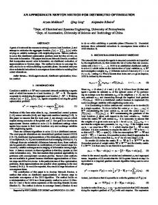
is straightforward. A special Newton-multilevel iterative method, along the lines discussed in Section 4, is used to solve the discrete equations. Details will be presented elsewhere. To illustrate the use of the Newton-multilevel iteration package and Algorithm Global, consider, as in [1], Section 4, the p ? n junction problem of the form (5.1) above. The functions v, w, and k are given, and the domain and boundary conditions are shown in Figure 5.1. Recall that the doping pro le k(x; y), and the solution gradient, ru(x; y), vary over several orders of magnitude in a small region near the junction, and there is a notable singularity due to the change in boundary conditions along the upper boundary.
u = �0
�
un = 0
Junction
un = 0
un = 0
u = �1
Fig. 5.1. p ? n junction problem with boundary conditions
We consider only the level-one nonuniform grid with n = 25 vertices (unknowns) and a (very poor) initial guess, u0 = 0. (The higher levels are less interesting.) We use Algorithm Global as in Section 4 with the modi cation (3.2)-(3.3) in line (7). The xk are computed by a sparse LU factorization of gk0 . The convergence trace is presented in Table 5.1. The relatively large number of iterations necessary in this experiment compared with the experiments reported in [1], Section 4, is a direct consequence of taking u0 = 0 rather than attempting to even roughly interpolate the boundary values �0 and �1 as we did before. This also leads to more searching (evals) than might otherwise be expected. As a cautionary remark, we report that failing to dynamically change K (i.e., taking Kk = K0 for all k) led to time overrun termination after k = 320, tk = 1:106(?4) and j gk j = 4:57(6) in the same experiment. REFERENCES [1] R. E. Bank and D. J. Rose, Parameter selection for Newton-like methods applicable to nonlinear partial di�erential equations, SIAM J. Numer. Anal., 17 (1980), pp. 806{822. 15
j g0 j = 4:738 � 106; evals � evaluations of g(u) k tk j gk j j uu ? uk?1 j =j uk j Evals
1 1.07(-4) 4.73(6) 2 7.30(-4) 4.70(6) 3 7.31(-3) 4.56(6) 4 7.05(-2) 3.41(6) 5 2.81(-2) 3.31(6) 6 2.30(-1) 2.21(6) 7 2.44(-1) 5.27(5) 8 9.31(-1) 5.88(4) 9 6.15(-2) 3.64(4) 10 1.52(-1) 3.11(4) 11 6.78(-1) 1.29(4) 12 9.81(-1) 5.73(3) 13 9.99(-1) 4.08(3) 14 7.39(-2) 3.79(3) 15 3.48(-1) 3.00(3) 16 8.71(-1) 1.75(3) 17 3.18(-1) 9.51(2) 18 8.95(-1) 5.18(2) 19 7.73(-1) 3.58(2) 20 7.66(-1) 1.03(2) 21 9.83(-1) 1.37(1) 22 1.a 1.44 23 1.a 1.57(-1) 24 1.a 7.67(-6) 25 1.a 4.27(-7) a 3 place rounding
9.28(3) 8.11(2) 9.16(1) 1.12(1) 1.33(1) 6.26(-1) 1.33 4.37(-1) 2.33 1.56 1.41 1.39(-1) 1.28(-1) 4.39(-1) 2.67(-1) 1.36(-1) 2.83(-1) 3.49(-2) 1.98(-2) 1.41(-2) 3.26(-3) 2.24(-4) 2.36(-5) 2.90(-6) 1.40(-10)
6 2 1 1 4 1 3 1 4 3 1 1 1 4 2 1 3 1 2 2 1 1 1 1 1
Table 5.1
[2] R. E. Bank and A. H. Sherman, PLTMG user's guide, Tech. Rep. CNA-152, Center for Numerical Analysis, University of Texas at Austin, 1979. [3] J. W. Daniel, The Approximate Minimization of Functionals, Prentice-Hall, Englewood Cli�s, NJ, 1971. [4] R. S. Dembo, S. C. Eisenstat, and T. Steihaug, Inexact-Newton methods, Tech. Rep. SOM Working Paper Series number 47, Yale University, 1981. [5] J. E. Dennis and J. J. Mor�e, A characterization of superlinear convergence and its application to quasi-Newton methods, Math. Comp., 28 (1974), pp. 549{560. , Quasi-Newton methods: motivation and theory, SIAM Rev., 19 (1977), pp. 46{89. [6] [7] W. Fichtner and D. J. Rose, On the numerical solution of nonlinear PDEs arising from semiconductor device modelling, in Elliptic Problem Solvers, (M. H. Schultz, ed.), Academic Press, New York, 1980. [8] , Numerical semiconductor device simulation, Tech. Rep. Technical memo, Bell Laboratories, 1981. [9] J. M. Ortega and W. C. Rheinboldt, Iterative Solution on Nonlinear Equations in Several Variables, Academic Press, New York, 1970. [10] I. W. Sandberg, One Newton-direction algorithms and di�eomorphisms, Tech. Rep. Technical memo, Bell Laboratories, 1980. [11] , Di�eomorphisms and Newton-direction algorithms, Bell Sys. Tech. J., (1981). [12] A. H. Sherman, On Newton-iterative methods for the solution of systems of nonlinear equations, SIAM J. Numer. Anal., 15 (1978), pp. 755{771. [13] A. Wouk, A Course of Applied Functional Analysis, J. Wiley and Sons, New York, 1979. 16