GLOBAL CONVERGENCE OF FILTER METHODS ... - Semantic Scholar

GLOBAL CONVERGENCE OF FILTER METHODS FOR NONLINEAR PROGRAMMING ´ ADEMIR A. RIBEIRO§ , ELIZABETH W. KARAS§ , AND CLOVIS C. GONZAGA¶ Abstract. We present a general filter algorithm that allows a great deal of freedom in the step computation. Each iteration of the algorithm consists basically in computing a point which is not forbidden by the filter, from the current point. We prove its global convergence, assuming that the step must be efficient, in the sense that, near a feasible non-stationary point, the reduction of the objective function is “large”. We show that this condition is reasonable, by presenting two classical ways of performing the step which satisfy it. In the first one, the step is obtained by the inexact restoration method of Mart´ınez and Pilotta. In the second, the step is computed by sequential quadratic programming. Key words. Filter methods, nonlinear programming, global convergence AMS subject classifications. 49M37, 65K05, 90C30

1. Introduction. We shall study the nonlinear programming problem minimize subject to

(P )

f0 (x) fE (x) = 0 fI (x) ≤ 0,

where the index sets E and I refer to the equality and inequality constraints respectively. Let the cardinality of E ∪ I be m, and assume that the functions fi : IRn → IR, i = 0, 1, . . . , m, are continuously differentiable. A nonlinear programming algorithm must deal with two different (and possibly conflicting) criteria, related respectively to optimality and to feasibility. Optimality is measured by the objective function f0 ; feasibility is typically measured by penalization of constraint violation, for instance, by the function h : IRn → IR+ , given by ° ° h(x) = °f + (x)° , (1.1) where k · k is an arbitrary norm and f + : IRn → IRm is defined by ½ fi+ (x) =

fi (x) max{0, fi (x)}

if i ∈ E if i ∈ I.

Both criteria must be optimized and the algorithm should follow a certain balance between them at every step of the iterative process. Several algorithms for nonlinear programming have been designed in which a merit function is a tool to guarantee global convergence [3, 10, 11, 19, 25]. As an alternative to merit function, Fletcher and Leyffer [7] introduced the so-called filter to globalize sequential quadratic programming type methods. Filter methods are based on the concept of dominance, borrowed from multi-criteria optimization. § Department of Mathematics, Federal University of Paran´ a, Cx. Postal 19081, 81531-980, Curitiba, PR, Brazil; e-mail :[email protected], [email protected]. ¶ Department of Mathematics, Federal University of Santa Catarina, Cx. Postal 5210, 88040-970, Florian´ opolis, SC, Brazil; e-mail : [email protected]. This author is supported by CNPq.

1

2

A. A. RIBEIRO, E. W. KARAS AND C. C. GONZAGA

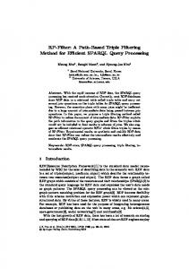
A filter algorithm defines a forbidden region, by memorizing pairs (f0 (xj ), h(xj )), chosen conveniently from former iterations and then avoids points dominated by these by the Pareto domination rule: y is dominated by x if, and only if, f0 (y) ≥ f0 (x) and h(y) ≥ h(x). Figure 1.1 shows a filter with four pairs, where we have simplified the notation by using x to represent the pair (f0 (x), h(x)). The point y is in the forbidden region and z is not.

h y j

x

z

f0 Fig. 1.1. A filter with four pairs.

The filter methods were also applied to sequential linear programming (SLP). The works of Chin and Fletcher [5] and Fletcher, Leyffer and Toint [8] present global convergence proofs of the method. For SQP-filter methods, global convergence has been proved by Fletcher, Leyffer and Toint [9], assuming that the quadratic subproblems are solved globally. Without this requirement, that is, allowing approximate solutions of the subproblems, Fletcher, Gould, Leyffer, Toint and Wächter [6] have also proved convergence to first-order critical points. Their approach uses a compositestep SQP method similar in spirit to the ones pioneered by Byrd [2] and Omojokun [21]. Another SQP-filter algorithm, using line search, was proposed by Wächter and Biegler [26], where global convergence was obtained. In the context of interior points, Ulbrich, Ulbrich and Vicente [23] have proposed a globally convergent primal-dual interior-point filter method. However, the filter entries have components that take into account the centrality and complementarity measures arising from interior-point techniques. The filter was also studied by Gonzaga, Karas and Vanti [12], in an algorithm that resembles the inexact restoration method of Mart´ınez and Pilotta [18, 19]. By suitable rules for building the filter they prove stationarity of all qualified accumulation points. The good performance of these methods [7, 15, 16] has motivated their use in other problems, like nonlinear systems of equations [13], unconstrained optimization [14] and nonsmooth convex constrained optimization [17]. This last work, by Karas, Ribeiro, Sagastizábal and Solodov, combines the ideas of the proximal bundle methods [22] with the filter strategy. Although we know that filter methods may suffer from the Maratos effect, we shall not discuss local convergence issues in this work. Some strategies can be found in [4, 24, 27] to ensure fast rate of convergence.

GLOBAL CONVERGENCE OF FILTER METHODS

3

In this paper, we propose a general filter algorithm that does not depend on the particular method used for the step computation. The only requirement is that the points generated must be acceptable for the filter and that near a feasible non-stationary point, the reduction of the objective function be large. This efficiency condition, stated ahead as Hypothesis H3, is the main tool of the global convergence analysis. It is a weaker version of the one introduced by Gonzaga, Karas and Vanti [12] in their inexact restoration filter method. Under this hypothesis, we prove that every sequence generated by the algorithm has at least one stationary accumulation point. Furthermore, we show how to compute the step in order to fulfill this hypothesis. One way to do this is by inexact restoration, for which H3 has proven in [12]. Another way for computing the step is by a sequential quadratic programming algorithm. We prove in this work that this approach also satisfies the efficiency condition H3. The paper is organized as follows. Our general filter algorithm and its convergence analysis are described in Section 2. In Section 3 we present the SQP method for computing the step and prove that Hypothesis H3 is satisfied. 2. The algorithm. In this section we present a general filter algorithm that allows a great deal of freedom in the step computation. Afterwards we state an assumption on the performance of the step, and prove that any sequence generated by the algorithm has a stationary accumulation point. In the next section we show that this condition is reasonable, by presenting a classical way of performing the step, satisfying this condition. ¡ j The ¢ algorithm constructs a sequence of filter sets F0 ⊂ F1 ⊂ · · · ⊂ Fk , composed of pairs ˜ j ∈ IR2 . We also mention in the algorithm the sets Fk ⊂ IRn , which are formally defined in f˜0 , h each step for clarity, but are never actually constructed. Algorithm 2.1. General filter algorithm model Given: x0 ∈ IRn , F0 = ∅, F0 = ∅, α ∈ (0, 1). k=0 repeat ¡ ¢ ˜ = f0 (xk ) − αh(xk ), (1 − α)h(xk ) . (f˜0 , h) S ˜ and define Set F¯k = Fk {(f˜0 , h)} S ˜ F¯k = Fk {x ∈ IRn | f0 (x) ≥ f˜0 , h(x) ≥ h}. Step: if xk is stationary, stop with success else, compute xk+1 ∈ / F¯k . Filter update: if f0 (xk+1 ) < f0 (xk ), Fk+1 = Fk , Fk+1 = Fk (f0 -iteration: the new entry is discarded) else, Fk+1 = F¯k , Fk+1 = F¯k (h-iteration: the new entry becomes permanent) k = k + 1. ˜ is temporarily introduced in the filter. After At the beginning of each iteration, the pair (f˜0 , h) the complete iteration, this entry will become permanent in the filter only if the iteration does not produce a decrease in f0 . Note that the forbidden region was slightly modified by subtracting the expression αh(xk ) from both filter pair components. This prevents the acceptance of trial pairs (f0 , h) arbitrarily close to old iterates (f0 (xj ), h(xj )). Figure 2.1 illustrates the effect of this modification which adds a small

4


margin around the border of region already defined by the Pareto domination rule. Now, all points above the dashed line are forbidden. h

y xj z

f0 Fig. 2.1. The filter margin.

In order to obtain our global convergence result, we shall assume that the algorithm generates an infinite sequence (xk )k∈IN in IRn and the following hypotheses are satisfied. H1. All the functions fi (·), i = 0, 1, . . . , m, are twice continuously differentiable. H2. The sequence (xk )k∈IN remains in a convex compact domain X ⊂ IRn . H3. Given a feasible non-stationary point x ¯ ∈ X, there exist M > 0 and a neighborhood V of x ¯ such that for any iterate xk ∈ V , f0 (xk ) − f0 (xk+1 ) ≥ M vk , n n oo ¡ ¢ ˜ j | f˜j , h ˜ j ∈ Fk . where vk = min 1, min h 0 The first ones are standard hypotheses, while the hypothesis H3 requires some discussion. With this hypothesis we are assuming that the step must be efficient, in the sense that, near a feasible non-stationary point, the reduction of the objective function is “large”. This assumption is a weaker version of the decrease condition introduced by Gonzaga, Karas and Vanti [12] who used (2.1)

oo n n ¢ ¡ ˜ j ∈ Fk , f˜j ≤ f0 (xk ) ˜ j | f˜j , h Hk = min 1, min h 0 0

instead of vk . Figure 2.2 shows the variables vk and Hk . We start with some relations which follow directly from the hypotheses and the construction of the algorithm. In the next section we shall state methods which satisfy Hypothesis H3. Lemma 2.2. Given k ∈ IN, the following statements hold: (i) Fk ⊂ Fk+1 (Inclusion property). (ii) xk+p ∈ / Fk+1 for all p ≥ 1. (iii) At least one of the two conditions below occurs: 1. f0 (xk+1 ) < f0 (xk ) − αh(xk ), k 2. h(xk+1 ) ¡< (1 − ¢ α)h(x ). ˜ ˜ ˜ (iv) h > 0 for all f0 , h ∈ Fk .


5

h

xk Hk vk f0 Fig. 2.2. The filter height vk and the filter slack Hk .

Proof. The first statement follows directly from the filter update criterion. By (i) and the ¯ we have Fk+1 ⊂ Fk+p ⊂ F¯k+p−1 . Then the second statement follows from xk+p ∈ definition of F, / ¯ Fk+p−1 . The third one is clear, since xk+1 ∈ / F¯k . Finally, note that if h(xk ) = 0, using (iii), we obtain f0 (xk+1 ) < f0 (xk ) − αh(xk ) = f0 (xk ), ˜ can be added to the filter only if that is, the iteration k is an f0 -iteration. Thus the pair (f˜0 , h) k ˜ h(x ) > 0, or equivalently if h > 0. This completes the proof. For the purpose of our analysis, we shall consider © ¡ ¢ ª (2.2) Ka = k ∈ IN | f0 (xk ) − αh(xk ), (1 − α)h(xk ) is added to the filter , the set of indices of h-iterations. First, we analyze what happens when this set is infinite. Lemma 2.3. If the set Ka is infinite, then K

h(xk ) →a 0. ¢ ¡ ¢ ¡ Proof. Given k, we denote f0 (xk ), h(xk ) by f0k , hk . Assume by contradiction that, for some δ > 0, the set © ª K = k ∈ Ka | h(xk ) ≥ δ is infinite. The continuity of (f0 , h), implied ¡ by H1, ¢ and the compactness assumption H2 ensure that there exists a convergent subsequence f0k , hk k∈K1 , K1 ⊂ K. Therefore, since α ∈ (0, 1), we can take indices j, k ∈ K1 , j < k such that °¡ ° ° k k ¢ ¡ j j ¢° ° f0 , h − f0 , h ° < αδ ≤ αh(xj ). This means that xk ∈ F¯j = Fj+1 , contradicting Lemma 2.2(ii) and completing the proof.

6


We now prove that the objective function decreases along the iterations, whenever the iterates stay near a non-stationary point. Lemma 2.4. Let x ¯ ∈ X be a non-stationary point. Then there exist k¯ ∈ IN and a neighborhood V of x ¯ such that whenever k > k¯ and xk ∈ V , the iteration k is an f0 -iteration, that is, k ∈ / Ka . Proof. If x ¯ is a feasible point, then by Hypothesis H3 there exist M > 0 and a neighborhood V of x ¯ such that for all xk ∈ V , f0 (xk ) − f0 (xk+1 ) ≥ M vk . Using Lemma 2.2(iv), we conclude that vk > 0, consequently f0 (xk+1 ) < f0 (xk ) and k is an f0 -iteration. Now, assume that x ¯ is infeasible and suppose by contradiction that there exists an infinite K K ¯. Since h is continuous, we have h(xk ) → h(¯ x). On the other set K ⊂ Ka such that xk → x K k hand, Lemma 2.3 ensures that h(x ) → 0. Thus h(¯ x) = 0, contradicting that x ¯ is infeasible and completing the proof. Our global convergence result is presented in the next theorem. Theorem 2.5. The sequence (xk )k∈IN has a stationary accumulation point. Proof. Let Ka be the set defined in (2.2). If Ka is infinite, then by H2 there exist K1 ⊂ Ka and K

x ¯ ∈ X such that xk →1 x ¯. From Lemma 2.4, x ¯ must be stationary. On the other hand, if K is finite, there exists k0 ∈ IN such that every iteration k ≥ k0 is an a ¡ ¢ f0 -iteration. Thus f0 (xk ) k≥k0 is decreasing and by H1 and H2, (2.3)

f0 (xk ) − f0 (xk+1 ) → 0.

Moreover, by construction, Fk = Fk0 for all k ≥ k0 . Therefore, the sequence (vk )k∈IN , defined in Hypothesis H3, satisfies (2.4) for all k ≥ k0 . If the set

vk = vk0 > 0 © ª K2 = k ∈ IN | αh(xk ) < f0 (xk ) − f0 (xk+1 ) K

is infinite, using (2.3), we conclude that h(xk ) →2 0. Otherwise, Lemma 2.2(iii) ensures that there exists k1 ∈ IN such that h(xk+1 ) < (1−α)h(xk ) for all k ≥ k1 , which in turn implies that h(xk ) → 0. Anyway, (xk )k∈IN has a feasible accumulation point x ¯. Now we prove that this point is stationary. k K Let K be a set of indices such that x → x ¯ and assume by contradiction that x ¯ is non-stationary. By Hypothesis H3, there exist k2 ∈ IN and M > 0 such that f0 (xk ) − f0 (xk+1 ) ≥ M vk for all k ∈ K, k ≥ k2 . This together with (2.4) contradicts (2.3), completing the proof. As we have seen above, the hypothesis H3 is crucial for the convergence analysis. It is a very strong assumption and we must show that there exist methods satisfying this condition. One of them is the inexact restoration method of Mart´ınez and Pilotta [19]. Gonzaga, Karas and Vanti [12] have proved in their inexact restoration filter method a condition that implies our hypothesis. We now discuss another way of performing the step, satisfying H3. It uses sequential quadratic programming and decomposes the step into its normal and tangential components.


7

3. Sequential quadratic programming. In this section we present an SQP method based on that proposed by Fletcher, Gould, Leyffer, Toint and Wächter [6], which computes the overall step in two phases. First, a feasibility phase aims at reducing the infeasibility measure h, satisfying a linear approximation of the constraints. Then an optimality phase computes a trial point reducing a quadratic model of the objective function in the linearization of the feasible set. We prove that this approach satisfies Hypothesis H3. The step computation. Given the current iterate xk and a trust-region radius ∆ > 0, we compute the step by solving the quadratic subproblem minimize subject to

(QPk )

mk (xk + d) xk + d ∈ L(xk ) kdk ≤ ∆,

where 1 mk (xk + d) = f0 (xk ) + ∇f0 (xk )T d + dT Bk d, 2

(3.1) with Bk symmetric, and (3.2)

© ª L(xk ) = xk + d ∈ IRn | fE (xk ) + AE (xk )d = 0, fI (xk ) + AI (xk )d ≤ 0 .

The matrix Bk may be chosen as an approximation of the Hessian of some Lagrangian function or any other symmetric matrix, provided that it remains uniformly bounded. See the hypothesis H6 below. The solution of (QPk ) yields a trial point xk + d∆ , that will be evaluated by the filter. To be accepted as the new iterate, this point must not be forbidden. In fact, we will see the step d∆ as the sum of two components, a feasibility step nk and a tangential (optimality) step t∆ . We now discuss each one of these steps. Feasibility step and compatibility of (QPk ). The feasibility step nk must satisfy the constraints of (QPk ) and has the purpose of reducing the infeasibility measure h. This can be done, for example, by nk = PL(xk ) (xk ) − xk , where PL(x) (·) is the projection onto the set L(x). However, we do not use this particular choice, but we shall assume a certain efficiency in this phase, given by the following hypothesis. H4. There exist constants δh > 0 and cn > 0 such that for all k ≥ 0 with h(xk ) ≤ δh , a step k n can be computed, satisfying ° k° °n ° ≤ cn h(xk ). This assumption means that the feasibility step must be reasonably scaled with respect to the constraints. In particular, nk = 0 whenever xk is feasible. This hypothesis is discussed by Mart´ınez [18], who presents a feasibility algorithm which satisfies it.

8


The step nk is only useful if it is not too close to the trust-region boundary because, otherwise, the tangential step is unlikely to produce a sufficient decrease in the model mk . We say that the subproblem (QPk ) is compatible when L(xk ) 6= ∅ and ° k° °n ° ≤ ξ∆, (3.3) where ξ ∈ (0, 1) is a constant. In our analysis, we shall consider z k = x k + nk

(3.4)

the point obtained in the feasibility phase. Note that, from (3.1) and (3.4), we have (3.5)

1 T mk (z k ) = mk (xk + nk ) = f0 (xk ) + ∇f0 (xk )T nk + nk Bk nk . 2

Tangential step. If the subproblem (QPk ) is compatible, we anticipate a satisfactory decrease in the model when performing a tangential step t∆ , approximate solution of the quadratic problem

(T Pk )

minimize subject to

¡

¢T ∇f0 (xk ) + Bk nk t + 12 tT Bk t AE (xk )t = 0 k k fI (xk ) + ° ° AI (x )(n + t) ≤ 0 °nk + t° ≤ ∆.

This problem is equivalent to (QPk ) with d = nk + t. Given the current iterate xk and a trust-region radius ∆ > 0, if (QPk ) is compatible, the trial point is xk + d∆ = z k + t∆ , where z k = xk + nk is the point which comes from the feasibility phase and t∆ is the tangential step. Restoration procedure. If the subproblem (QPk ) is not compatible, the algorithm calls a restoration procedure, whose aim is to obtain a point xk+1 ∈ / F¯k with h(xk+1 ) < h(xk ), where the function h is the infeasibility measure defined by (1.1). This can be done by taking steps of some algorithm for solving the problem minimize h(x) . x ∈ IRn We can now summarize the above discussion in the following algorithm for the step computation. After stating the algorithm we shall make some comments about its features.


9

Algorithm 3.1. Computation of xk+1 ∈ / F¯k n k ¯ Data: x ∈ IR , the current filter Fk , 0 < ∆min < ∆max , ∆ ∈ [∆min , ∆max ] and cp , ξ, η, γ ∈ (0, 1). if L(xk ) = ∅, use the restoration procedure to obtain xk+1 ∈ / F¯k . else compute a feasibility step nk such that xk + nk ∈ L(xk ) k+1 repeat°(while is not obtained) ° the point x k° ° if n > ξ∆, use the restoration procedure to obtain xk+1 ∈ / F¯k . determine Bk+1 symmetric else, compute the tangential step t∆ as above and define d∆ = nk + t∆ k set ared = f0 (xk ) − f0 (x pred = mk (xk ) − mk (xk + do∆ ) n + d∆ ) and © k ª ¡ ¢2 if x + d∆ ∈ F¯k or pred ≥ cp h(xk ) and ared < η pred ∆ = γ∆ else xk+1 = xk + d∆ determine Bk+1 symmetric ∆k = ∆ Algorithm 3.1 was inspired in the SQP-filter algorithm proposed by Fletcher, Gould, Leyffer, Toint and Wächter [6]. However, there exist some differences between them, which we now point out. The first one is that here the step computation is made separately from the main filter algorithm, presented in Section 2. This simplifies the study of the step properties and leaves the convergence analysis of the main algorithm in a clean framework. Another difference is in the trustregion radius. Algorithm 3.1 starts with a radius ∆ ∈ [∆min , ∆max ], where ∆min , ∆max > 0 are constants. This procedure is not used in [6], making the convergence proofs involved. To overcome some difficulties they impose a condition like ° k° °n ° ≤ c∆1+µ , where c > 0 and µ ∈ (0, 1), to accept the normal step and to proceed with the tangential step. In our algorithm, this condition is replaced by (3.3), that is, ° k° °n ° ≤ ξ∆, where ξ ∈ (0, 1) is a constant. This requirement is usual in the composite-step approaches that we are considering. We mention that the choice of a minimum radius ∆min may cause practical disadvantages, like the rejection of many trial points before the progress of the algorithm. On the other hand, it simplifies the analysis and enhances the chance of taking a pure Newton step. Remarks. At iteration k, we denote by d∆ the trial step obtained with the trust-region radius ∆ ≥ ∆k . The point xk+1 can be computed in two different ways: by means of a restoration procedure or by xk+1 = xk + d∆k . We also have two possibilities for rejecting the trial step d∆ : (3.6)

xk + d∆ ∈ F¯k

10


or (3.7)

¡ ¢2 pred ≥ cp h(xk ) and ared < η pred.

In both cases the trust-region radius is reduced and a new step is computed. Thus, in order to accept the step d∆ , it is not enough to pass the filter criterion. It also must ensure a sufficient decrease in the objective function whenever the predicted reduction is more significant than the constraint violation. In particular, if all iterates are feasible, the first inequality in (3.7) will be always true, because nk = 0 in this case. Furthermore, if ared ≥ η pred, then xk + d∆ ∈ / F¯k . So, the step acceptance criterion reduces to ared ≥ η pred and the algorithm may be viewed as a classical unconstrained trust-region method. We now prove that Hypothesis H3 is satisfied if Algorithm 2.1 is applied to problem (P ) and the step is obtained by Algorithm 3.1. For that, we shall introduce a function used as a stationarity measure. Given x, z ∈ X and the set L(x) defined in (3.2), we denote (3.8)

dc (x, z) = PL(x) (z − ∇f0 (x)) − z

the projected gradient direction and the function ϕ : IRn × IRn → IR, given by  c  −∇f0 (x)T d (x, z) if dc (x, z) 6= 0, kdc (x, z)k ϕ(x, z) = (3.9)  0 otherwise, the stationarity measure. According to [12] we have, at a feasible point x ¯, that the KKT conditions are equivalent to dc (¯ x, x ¯) = 0. Furthermore, if x ¯ is non-stationary, then ϕ(¯ x, x ¯) > 0. The projected gradient direction given above is based on a direction introduced by Mart´ınez and Svaiter [20] to define a new optimality condition, called AGP property (Approximate Gradient Projection), that implies, and is strictly stronger than, Fritz-John optimality conditions. Unlike the KKT conditions, it is satisfied by local minimizers of nonlinear programming problems, independently of constraint qualifications. Note. Let us give an interpretation for the direction dc (x, z) when z ∈ L(x) (which is the case in the algorithm). It is an approximation to dB (z) = PL(x) (z − ∇f0 (z)) − z. This is the projected Cauchy direction defined by Bertsekas [1] for the minimization of f0 (·) in L(x) and dB (z) = 0 implies that z is stationary for this problem. If, in addition, z is feasible for (P ) it is also stationary for (P ). The direction dc (x, z) may be a good descent direction for (P ) if ∇f0 (x) ∇f0 (z) ≈ , k∇f0 (x)k k∇f0 (z)k but otherwise it may be meaningless (possibly null). If dc (x, z) 6= 0, we consider dc1 = To continue our analysis we define the generalized Cauchy step given by  ° ° © ª  argmin mk (z k + λdc1 ) | °z k + λdc1 − xk ° ≤ ∆ if dc (xk , z k ) 6= 0, λ≥0 tc =  0 otherwise,

dc (x, z) . kdc (x, z)k


11

and we assume the following hypotheses related to Algorithm 3.1. H5. If the subproblem (QPk ) is compatible, then the model decrease at the tangential step t∆ satisfies mk (z k ) − mk (z k + t∆ ) ≥ mk (z k ) − mk (z k + tc ). H6. The matrices Bk are uniformly bounded, that is, there exists a constant β > 0 such that kBk k ≤ β for all k ≥ 0. The assumption H5 says that the tangential step must be at least as good as the generalized Cauchy step tc . We also consider a very standard condition on the Hessians Bk , stated in Hypothesis H6. We start our task by evaluating the infeasibility measure before and after the trial step. Lemma 3.2. Suppose that Hypotheses H1 and H2 hold. There exists a constant ch > 0 such that for any xk ∈ X and ∆ > 0 so that the problem (QPk ) is compatible, h(xk ) ≤ ch ∆

and

h(xk + d∆ ) ≤ ch ∆2 ,

where d∆ is the trial step obtained by Algorithm 3.1. Proof. It follows from Hypotheses H1 and H2 that there exists a constant ch > 0 such that ° 2 ° °∇ fi (x)° ≤ ch k∇fi (x)k ≤ ch and (3.10) for all x ∈ X and i = 1, . . . , m. Consider xk ∈ X and ∆ > 0 so that the problem (QPk ) is compatible. Thus the feasibility step nk and the trial step d∆ were computed by Algorithm 3.1. Taking, without loss of generality, the norm k·k∞ in (1.1) and using the fact that xk + nk ∈ L(xk ), we conclude that h(xk ) = |fi (xk )| = | − ∇fi (xk )T nk | for some i ∈ E, or h(xk ) = fi (xk ) ≤ −∇fi (xk )T nk for some i ∈ I. Hence, from the Cauchy-Schwarz inequality, (3.10) and the trust-region boundedness of nk , we obtain ° °° ° h(xk ) ≤ °∇fi (xk )° °nk ° ≤ ch ∆, proving the first claim in the lemma. To prove the other inequality, note that by Taylor’s theorem and the fact that xk + d∆ ∈ L(xk ), fi (xk + d∆ ) =

1 T 2 d ∇ fi (xk + θi d∆ )d∆ , 2 ∆

fi (xk + d∆ ) ≤

1 T 2 d ∇ fi (xk + θi d∆ )d∆ , 2 ∆

for i ∈ E, and

12


for i ∈ I, where θi ∈ (0, 1). Because the trust-region radius is bounded, we may assume without loss of generality that the trial points also remain in the compact set X. Thus, from (3.10), the Cauchy-Schwarz inequality and since kd∆ k ≤ ∆, h(xk + d∆ ) ≤ ch ∆2 , completing the proof. We next assess the model and the objective function growth in the feasibility step computed by Algorithm 3.1. Lemma 3.3. Suppose that Hypotheses H1, H2, H4 and H6 hold. Given a feasible point x ¯ ∈ X, k k k k there exist N > 0 and a neighborhood V of x ¯ such that if x ∈ V and z = x + n , then 1 1 ¯ ¯ (i) ¯mk (xk ) − mk (z k )¯ ≤ N h(xk ). ¯ ¯ (ii) ¯f0 (xk ) − f0 (z k )¯ ≤ N h(xk ). Proof. Let δh and cn be the constants given by H4, and β given by H6. Consider the constant cg = max {k∇f0 (x)k | x ∈ X}, whose existence is ensured by H1 and H2. Since h(¯ x) = 0 and h is continuous, there exists a neighborhood V1 of x ¯ such that if xk ∈ V1 , then (3.11)

h(xk ) ≤ δh

¢2 1 2¡ βcn h(xk ) ≤ cg cn h(xk ). 2

and

By (3.5), we have 1 T mk (z k ) = mk (xk ) + ∇f0 (xk )T nk + nk Bk nk . 2 Using the Cauchy-Schwarz inequality, H4 and H6, we obtain |mk (xk ) − mk (z k )| ≤ ≤

° °2 ° ° cg °nk ° + 21 β °nk ° ¡ ¢2 cg cn h(xk ) + 21 βc2n h(xk ) .

From the second inequality in (3.11), it follows that |mk (xk ) − mk (z k )| ≤ 2cg cn h(xk ). On the other hand, by Hypotheses H1 and H2, there exists a constant L > 0 such that ° ° |f0 (xk ) − f0 (z k )| ≤ L °xk − z k ° . This together with H4 yields |f0 (xk ) − f0 (z k )| ≤ Lcn h(xk ). Taking N = max {2cg cn , Lcn }, we complete the proof.


13

Remark. As we have seen in the proof of Lemma 3.3, h(xk ) ≤ δh whenever xk ∈ V1 . Therefore, given a neighborhood V ⊂°V1 ,°if xk ∈ V , the hypothesis H4 is applicable, that is, the step nk can be computed and satisfies °nk ° ≤ cn h(xk ). Now we prove that the model and the objective function reductions are large near a feasible non-stationary point, if we ignore the filter. The first lemma looks only at the tangential step, while the second lemma considers the whole step (feasibility and tangential). Lemma 3.4. Suppose that Hypotheses H1, H2, H4-H6 hold. Let x ¯ ∈ X be a feasible nonstationary point and η¯ ∈ (0, 1). Consider the neighborhood V1 and the constant ∆min given by Lemma 3.3 and Algorithm 3.1, respectively. Then there exist constants ∆ρ ∈ (0, ∆min ], c˜ > 0 and a neighborhood V2 ⊂ V1 of x ¯ such that whenever xk ∈ V2 , z k = xk + nk and a tangential trial step t∆ is obtained by the algorithm, we have (i) mk (z k ) − mk (z k + t∆ ) ≥ c˜∆0 for all ∆, ∆0 such that ∆0 ≤ min {∆, ∆ρ }. ¡ ¢ (ii) f0 (z k ) − f0 (z k + t∆ ) ≥ η¯ mk (z k ) − mk (z k + t∆ ) for all ∆ ∈ (0, ∆ρ ]. Proof. Let ∆ > 0 and λ∆0 = (1 − ξ)∆0 , where ξ is given by (3.3) and ∆0 ≤ ∆. First, note that the vector dc1 , defined in H5, satisfies kdc1 k = 1. Consequently ° k ° ° ° ° ° °z + λ∆0 dc1 − xk ° = °nk + λ∆0 dc1 ° ≤ °nk ° + λ∆0 ≤ ξ∆ + (1 − ξ)∆0 ≤ ∆. Using the assumption on the Cauchy point H5, we obtain mk (z k ) − mk (z k + t∆ ) ≥ mk (z k ) − mk (z k + tc ) ≥ mk (z k ) − mk (z k + λ∆0 dc1 ). Developing the quadratic model (3.1) in the right hand side, we conclude that ¶ µ 1 T mk (z k ) − mk (z k + t∆ ) ≥ λ∆0 −∇f0 (xk )T dc1 − nk Bk dc1 − λ∆0 dc1 T Bk dc1 . 2 By (3.9), ϕ(xk , z k ) = −∇f0 (xk )T dc1 and by H6, kBk k ≤ β. Hence µ ¶ ° ° 1 mk (z k ) − mk (z k + t∆ ) ≥ λ∆0 ϕ(xk , z k ) − °nk ° β − λ∆0 β . (3.12) 2 Since°x ¯ is x, x ¯) > 0. Using the fact ° feasible non-stationary, the continuous function ϕ satisfies ϕ(¯ that °nk ° ≤ cn h(xk ) by H4, we conclude that there exist a neighborhood V2 of x ¯ and ∆0 ∈ (0, ∆min ] such that for any xk ∈ V2 and ∆0 ∈ (0, ∆0 ], ϕ(xk , z k ) ≥

1 ϕ(¯ x, x ¯) 2

and

° k° °n ° β + 1 λ∆0 β ≤ 1 ϕ(¯ x, x ¯). 2 4

Thus, by (3.12), we obtain for ∆0 ≤ min {∆, ∆0 }, mk (z k ) − mk (z k + t∆ ) ≥

1 1 λ∆0 ϕ(¯ x, x ¯) = (1 − ξ)ϕ(¯ x, x ¯)∆0 . 4 4

This proves (i) for any ∆ρ ≤ ∆0 and c˜ = 14 (1 − ξ)ϕ(¯ x, x ¯). To prove (ii), note that by the mean value theorem, def

aredzk = f0 (z k ) − f0 (z k + t∆ ) = −∇f0 (z k + θt∆ )T t∆ ,

14


for some θ ∈ (0, 1). On the other hand, 1 def predzk = mk (z k ) − mk (z k + t∆ ) = −∇f0 (xk )T t∆ − tT∆ Bk nk − tT∆ Bk t∆ . 2 By H1 and H2, we can apply the mean value inequality to ∇f0 to conclude that there exists a constant L > 0 such that ° ° ° ° °∇f0 (xk ) − ∇f0 (z k + θt∆ )° ≤ L °z k − xk + θt∆ ° , so, using the facts that kBk k ≤ β and kt∆ k ≤ ∆, we obtain ° ° ° ° 2 |aredzk − predzk | ≤ L °z k − xk + θt∆ ° kt∆ k + β °nk ° kt∆ k + 12 β kt∆ k ° k° ° ° ≤ L °n ° ∆ + L∆2 + β °nk ° ∆ + 21 β∆2 ° ° ¡ ¢ = (L + β) °nk ° ∆ + L + 21 β ∆2 . We can restrict the neighborhood V2 , if necessary, and take ∆ρ ≤ ∆0 such that for any xk ∈ V2 and ∆ ∈ (0, ∆ρ ], ° ° ¡ ¢ L + 21 β ∆ (L + β) °nk ° 1 − η¯ 1 − η¯ ≤ and ≤ . c˜ 2 c˜ 2 Consequently, using (i) with ∆0 = ∆, ° ° ¡ ¢ ¯ ¯ ¯ ¯ ¯ ¯ aredzk − predzk ¯ (L + β) °nk ° ∆ + L + 12 β ∆2 ¯ aredzk ¯ ¯ ¯ ¯ ≤ 1 − η¯, ¯≤ ¯ pred k − 1¯ = ¯ predzk c˜∆ z completing the proof. In the next lemma we extend for the whole step the properties of the tangential step near a feasible non-stationary point. Lemma 3.5. Suppose that Hypotheses H1, H2, H4-H6 hold. Let x ¯ ∈ X be a feasible nonstationary point and 0 < η < 1. Consider the constant γ given in Algorithm 3.1, the neighborhood V2 and the constant ∆ρ given in Lemma 3.4. Then there exists a neighborhood V3 ⊂ V2 of x ¯ such that whenever xk ∈ V3 , z k = xk + nk and a tangential trial step t∆ is obtained by the algorithm, we have for all ∆ ∈ [γ 2 ∆ρ , ∆ρ ], (i) mk (xk ) − mk (z k + t∆ ) ≥ 12 c˜∆, ¡ ¢ (ii) f0 (xk ) − f0 (z k + t∆ ) ≥ η mk (xk ) − mk (z k + t∆ ) . η¯ − η Proof. Let η¯ ∈ (η, 1) and τ = . Consider the constants N and c˜ given by Lemmas 3.3 and η¯ + η 3.4, respectively, and V3 ⊂ V2 a neighborhood of x ¯ such that for all x ∈ V3 , ½ ¾ 1 2 (3.13) N h(x) ≤ min c˜γ ∆ρ , τ η¯c˜γ 2 ∆ρ . 2 Hence, if xk ∈ V3 and ∆ ∈ [γ 2 ∆ρ , ∆ρ ], we can apply Lemma 3.3 to conclude that ¯ ¯ ¯mk (xk ) − mk (z k )¯ ≤ N h(xk ) ≤ 1 c˜γ 2 ∆ρ ≤ 1 c˜∆. 2 2

15


It follows from this and Lemma 3.4(i) with ∆0 = ∆ that mk (xk ) − mk (z k + t∆ ) = mk (xk ) − mk (z k ) + mk (z k ) − mk (z k + t∆ ) ≥

1 c˜∆, 2

proving (i). (ii) Applying again Lemmas 3.3 and 3.4 together with (3.13), we obtain ¯ ¯ ¡ ¢ ¯f0 (xk ) − f0 (z k )¯ ≤ N h(xk ) ≤ τ η¯c˜γ 2 ∆ρ ≤ τ η¯c˜∆ ≤ τ f0 (z k ) − f0 (z k + t∆ ) and ¡ ¢ mk (xk ) − mk (z k ) ≤ N h(xk ) ≤ τ c˜γ 2 ∆ρ ≤ τ c˜∆ ≤ τ mk (z k ) − mk (z k + t∆ ) . Consequently (3.14)

f0 (xk ) − f0 (z k + t∆ ) = ≥

f0 (xk ) − f0 (z k ) + f0 (z k ) − f0 (z k + t∆ ) ¡ ¢ (1 − τ ) f0 (z k ) − f0 (z k + t∆ )

and (3.15)

mk (xk ) − mk (z k + t∆ ) = ≤

mk (xk ) − mk (z k ) + mk (z k ) − mk (z k + t∆ ) ¡ ¢ (1 + τ ) mk (z k ) − mk (z k + t∆ ) .

Therefore, if xk ∈ V3 and ∆ ∈ [γ 2 ∆ρ , ∆ρ ], using (3.14), (3.15) and Lemma 3.4(ii), we obtain ¡ ¢ f0 (xk ) − f0 (z k + t∆ ) ≥ (1 − τ )¯ η mk (z k ) − mk (z k + t∆ ) ¢ (1 − τ )¯ η¡ ≥ mk (xk ) − mk (z k + t∆ ) (1 ¡ + τ) ¢ = η mk (xk ) − mk (z k + t∆ ) , completing the proof. In the next two results we shall use the filter slack Hk , defined in (2.1). First we show that, near a feasible non-stationary point, the rejection of a step is due to a large increase of the infeasibility. Lemma 3.6. Suppose that Hypotheses H1, H2, H4-H6 hold. Let x ¯ ∈ X be a feasible nonstationary point and consider the constants γ and ∆ρ given by Algorithm 3.1 and Lemma 3.4, respectively and the neighborhood V3 given by Lemma 3.5. Then there exists a neighborhood V ⊂ V3 of x ¯ such that whenever xk ∈ V , z k = xk + nk and a tangential trial step t∆ is obtained by the algorithm, we have h(z k + t∆ ) ≥ Hk for any ∆ ∈ [γ 2 ∆ρ , ∆ρ ] that was rejected by Algorithm 3.1. Proof. Let α, η, N and c˜ be the constants given by Algorithms 2.1, 3.1 and Lemmas 3.3, 3.4, respectively. Consider V ⊂ V3 a neighborhood of x ¯ such that for all x ∈ V , (3.16)

N h(x) ≤

1 2 c˜γ ∆ρ 2

and

αh(x) ≤

1 η˜ cγ 2 ∆ρ . 2

16


Hence, if xk ∈ V and ∆ ∈ [γ 2 ∆ρ , ∆ρ ], we can apply Lemma 3.3 to obtain ¯ ¯ ¯mk (xk ) − mk (z k )¯ ≤ N h(xk ) ≤ 1 c˜γ 2 ∆ρ ≤ 1 c˜∆, 2 2 which together with Lemma 3.4 yields (3.17)

mk (xk ) − mk (z k + t∆ ) ≥

1 1 c˜∆ ≥ c˜γ 2 ∆ρ . 2 2

Using Lemma 3.5, (3.16) and (3.17), we obtain f0 (xk ) − f0 (z k + t∆ ) ≥ ≥ ≥

¡ ¢ η mk (xk ) − mk (z k + t∆ ) 1 cγ 2 ∆ρ 2 η˜ αh(xk ).

Since z k + t∆ = xk + d∆ , it follows that (3.18)

¡ ¢ f0 (xk ) − f0 (xk + d∆ ) ≥ η mk (xk ) − mk (xk + d∆ )

and (3.19)

f0 (xk + d∆ ) ≤ f0 (xk ) − αh(xk ).

Therefore, if the trial step d∆ was rejected by Algorithm 3.1, then xk + d∆ ∈ F¯k because of (3.18). We thus conclude from (3.19) that h(z k + t∆ ) ≥ Hk , completing the proof. We now prove the main result of this section: Hypothesis H3 is satisfied. Indeed, we give a sufficient condition to ensure H3. As we saw in Theorem 2.5, this hypothesis was crucial in the convergence analysis of Section 2. For the purpose of our analysis, we shall consider the set of restoration iterations ° ° © ª Kr = k ∈ IN | L(xk ) = ∅ or °nk ° > ξ∆k , (3.20) where L(xk ) is defined by (3.2). We also assume the following hypothesis. H7. Every feasible accumulation point x ¯ ∈ X of (xk )k∈IN satisfies the Mangasarian-Fromovitz constraint qualification, namely, the gradients ∇fi (¯ x) for i ∈ E are linearly independent, and there exists a direction d ∈ IRn such that AE (¯ x)d = 0 and AI¯ (¯ x)d < 0, where I¯ = {i ∈ I | fi (¯ x) = 0}. Theorem 3.7. Suppose that Algorithm 2.1 is applied to problem (P ), with the step computed by Algorithm 3.1, and that Hypotheses H1, H2, H4-H7 hold. Given a feasible non-stationary point x ¯ ∈ X, there exist M > 0 and a neighborhood V of x ¯ such that if xk ∈ V , then p f0 (xk ) − f0 (xk+1 ) ≥ M Hk . √ In particular, since Hk ≥ vk , the hypothesis H3 is satisfied.


17

Proof. Let x ¯ be a feasible non-stationary point. Consider the neighborhood V given by Lemma 3.6 and the constant ∆ρ given by Lemma 3.4. Without loss of generality, we can assume that ½ ¾ γ2 ξ c˜ c˜ η˜ c (3.21) ∆ρ ≤ min , , , , ch cn 2N 2cp 2α where α is the constant given in Algorithm 2.1, ξ, γ, cp and η are given in Algorithm 3.1, cn is given in Hypothesis H4 and ch , N and c˜ are given by Lemmas 3.2, 3.3 and 3.4, respectively. By the constraint qualification hypothesis H7, we can assume that if xk ∈ V , then L(xk ) 6= ∅. Thus, Algorithm 3.1 starts with the radius ∆ ≥ ∆min and ends with ∆k = γ r ∆, where r is the number of times that the radius was reduced in the algorithm. We shall consider two cases, respectively with ∆k ≥ γ 2 ∆ρ and ∆k < γ 2 ∆ρ . First case: ∆k ≥ γ 2 ∆ρ . In this case, using the hypothesis H4 and restricting the neighborhood V , if necessary, we have ° k° °n ° ≤ cn h(xk ) ≤ ξγ 2 ∆ρ ≤ ξ∆k . So, Algorithm 3.1 does not enter the restoration phase during the iteration k, that is, k ∈ / Kr . Therefore, applying Lemma 3.4(i) with ∆0 = γ 2 ∆ρ , we obtain (3.22)

mk (z k ) − mk (xk+1 ) = mk (z k ) − mk (z k + t∆k ) ≥ c˜γ 2 ∆ρ .

On the other hand, by Lemma 3.3(i), ¯ ¯ ¯mk (xk ) − mk (z k )¯ ≤ N h(xk ). (3.23) We can restrict again the neighborhood V , if necessary, so that (3.24)

N h(xk ) ≤

1 2 c˜γ ∆ρ 2

,

¡ ¢2 1 cp h(xk ) ≤ c˜γ 2 ∆ρ 2

and

h(xk ) ≤ 1.

By (3.22)-(3.24), we have def

predk = mk (xk ) − mk (xk+1 ) ≥

¡ ¢2 1 2 c˜γ ∆ρ ≥ cp h(xk ) . 2

Then the mechanism of Algorithm 3.1 and the fact that Hk ≤ 1 imply that (3.25)

def

f0 (xk ) − f0 (xk+1 ) = aredk ≥ η predk ≥

p 1 1 η˜ cγ 2 ∆ρ ≥ η˜ cγ 2 ∆ ρ H k . 2 2

Second case: now, assume that ∆k < γ 2 ∆ρ . In this case we shall analyze two possibilities. In the first one, we suppose that h(xk + d∆ ) ≥ Hk for all ∆ ≤ γ∆ρ such that the trial step d∆ has been ˜ = ∆k . Since ∆k < ∆min , the trial step d˜ = d ˜ was computed. Furthermore, computed. Let ∆ ∆ γ k ˜ ˜ h(x + d) ≥ Hk because ∆ < γ∆ρ . So, using Lemma 3.2 and the definition of Hk , it follows that (3.26)

˜ ≥ γ 2 Hk ≥ γ 2 h(xk ). ˜ 2 ≥ γ 2 h(xk + d) ch ∆2k = ch γ 2 ∆

From Hypothesis H4, (3.21) and (3.26), we obtain ° k° °n ° ≤ cn h(xk ) ≤ cn ch ∆2k ≤ ξ∆k , γ2

18


meaning that Algorithm 3.1 does not enter the restoration phase during the iteration k, that is, k∈ / Kr . Therefore, by Lemma 3.4(i) with ∆0 = ∆k , we have (3.27)

mk (z k ) − mk (xk+1 ) = mk (z k ) − mk (z k + t∆k ) ≥ c˜∆k .

Moreover, (3.23) remains true in this case and together with (3.21) and (3.26) yields (3.28)

¯ ¯ ¯mk (xk ) − mk (z k )¯ ≤ N h(xk ) ≤ N ch ∆2k ≤ 1 c˜∆k . γ2 2

Combining (3.27) and (3.28), we obtain predk = mk (xk ) − mk (xk+1 ) ≥

(3.29)

1 c˜∆k . 2

By (3.21), (3.24) and (3.26), predk ≥

¡ ¢2 cp ch 2 ∆ ≥ cp h(xk ) ≥ cp h(xk ) . γ2 k

Thus, the mechanism of Algorithm 3.1, (3.26) and (3.29) imply that (3.30)

f0 (xk ) − f0 (xk+1 ) = aredk ≥ η predk ≥

1 η˜ cγ p η˜ c∆k ≥ √ Hk . 2 2 ch

Let us see now the second possibility, that is, there exists ∆ ≤ γ∆ρ such that h(xk + d∆ ) < Hk . ˆ be the first ∆ satisfying such a condition. We shall show that ∆ ˆ = ∆k . Let d¯ = d∆ Let ∆ ¯ be the ˆ ¯ = ∆ . We claim that trial step obtained with ∆ γ ¯ ≥ Hk . h(xk + d)

(3.31)

¯ ≤ γ∆ρ , the definition of ∆ ˆ ensures the claim. On the other hand, if ∆ ¯ > γ∆ρ , then Indeed, if ∆ ¯ ∈ [γ 2 ∆ρ , ∆ρ ] and, applying Lemma 3.6, we have ∆ ¯ = h(z k + t∆ h(xk + d) ¯ ) ≥ Hk . So, the inequality (3.31) holds. As above, we can prove that ˆ 2 ≥ γ 2 Hk ≥ γ 2 h(xk ) ch ∆

(3.32) and (3.33)

def

k k pred∆ ˆ) ≥ ˆ = mk (x ) − mk (z + t∆

1 ˆ c˜∆. 2

Now, by the same reasoning as in the proof of Lemma 3.5(ii), using (3.32) and (3.33), we obtain (3.34)

def

k k ared∆ ˆ ) ≥ η pred∆ ˆ ≥ ˆ = f0 (x ) − f0 (z + t∆

1 ˆ η˜ c∆, 2


19

which together with (3.21) and (3.32) yields (3.35)

ared∆ ˆ >

αch ˆ 2 ∆ ≥ αh(xk ). γ2

ˆ and (3.35) ensure that z k + t ˆ is accepted by the filter. Therefore, using (3.34), The definition of ∆ ∆ k+1 we conclude that z k + t∆ . Moreover, (3.32) and (3.34) imply that ˆ =x f0 (xk ) − f0 (z k + t∆ ˆ) ≥

1 ˆ η˜ cγ p Hk , η˜ c∆ ≥ √ 2 2 ch

that is, (3.36)

η˜ cγ p f0 (xk ) − f0 (xk+1 ) ≥ √ Hk . 2 ch

Since (3.25), (3.30) and (3.36) run out all possibilities, by defining ¾ ½ η˜ cγ 1 2 η˜ cγ ∆ρ , √ , M = min 2 2 ch we complete the proof. 4. Conclusions. In this work we have studied filter methods for nonlinear programming. These methods seem to be a successful strategy for globalizing algorithms without the use of merit functions. Since its appearance in 1997, the filter technique has been applied to many problems, including sequential linear programming (SLP), sequential quadratic programming (SQP), inexact restoration, interior-point methods, nonlinear systems of equations, unconstrained optimization and nonsmooth convex constrained optimization. Our purpose here was to present a general globally convergent filter algorithm that leaves the step computation separate from the main algorithm. This technique cleans the convergence analysis and accepts any method for computing the step, as long as this internal algorithm is efficient in the sense that the hypothesis H3, is satisfied. For completeness, we have shown that there are methods which satisfy the referred hypothesis. Acknowledgements. We thank the referees for their valuable comments and suggestions which very much improved this paper. REFERENCES [1] D. P. Bertsekas, Nonlinear Programming, Athena Scientific, Belmont, Massachusetts, 1995. [2] R. H. Byrd, Robust trust region methods for constrained optimization. Third SIAM Conference on Optimization, 1987. [3] R. H. Byrd, J. C. Gilbert, and J. Nocedal, A trust region method based on interior point techniques for nonlinear programming, Mathematical Programming, 89 (2000), pp. 149–185. [4] C. M. Chin, A local convergence theory of a filter line search method for nonlinear programming, tech. report, Numerical Optimization Report, Department of Statistics, University of Oxford, England, January 2003. [5] C. M. Chin and R. Fletcher, On the global convergence of an SLP-filter algorithm that takes EQP steps, Mathematical Programming, 96 (2003), pp. 161–177. ¨ chter, Global convergence of a trust-region [6] R. Fletcher, N. Gould, S. Leyffer, P. Toint, and A. Wa SQP-filter algorithm for general nonlinear programming, SIAM J. Optimization, 13 (2002), pp. 635–659.

20


[7] R. Fletcher and S. Leyffer, Nonlinear programming without a penalty function, Mathematical Programming - Ser. A, 91 (2002), pp. 239–269. [8] R. Fletcher, S. Leyffer, and P. L. Toint, On the global convergence of an SLP-filter algorithm, Tech. Report NA/183, Dundee University, Dept. of Mathematics, 1998. [9] , On the global convergence of a filter-SQP algorithm, SIAM J. Optimization, 13 (2002), pp. 44–59. [10] D. M. Gay, M. L. Overton, and M. H. Wright, A primal-dual interior method for nonconvex nonlinear programming, in Advances in Nonlinear Programming, Y. Y, ed., Kluwer Academic Publishers, Dordretch, 1998, pp. 31–56. [11] F. A. M. Gomes, M. C. Maciel, and J. M. Mart´ınez, Nonlinear programming algorithms using trust regions and augmented Lagrangians with nonmonotone penalty parameters, Mathematical Programming, 84 (1999), pp. 161–200. [12] C. C. Gonzaga, E. W. Karas, and M. Vanti, A globally convergent filter method for nonlinear programming, SIAM J. Optimization, 14 (2003), pp. 646–669. [13] N. I. M. Gould, S. Leyffer, and P. L. Toint, A multidimensional filter algorithm for nonlinear equations and nonlinear least-squares, SIAM Journal on Optimization, 15 (2005), pp. 17–38. [14] N. I. M. Gould, C. Sainvitu, and P. L. Toint, A filter-trust-region method for unconstrained optimization, SIAM Journal on Optimization, 16 (2006), pp. 341–357. [15] N. I. M. Gould and P. L. Toint, The filter idea and its application to the nonlinear feasibility problem, in Proceedings of the 20th Biennal Conference on Numerical Analysis, D. F. Griffiths and G. A. Watson, eds., Scotland, June 2003, pp. 73–79. [16] , FILTRANE, a fortran 95 filter-trust-region package for solving nonlinear feasibility problems, tech. report, CCLRC Rutherford Appleton Laboratory, England, September 2003. ´ bal, and M. Solodov, A bundle-filter method for nonsmooth [17] E. W. Karas, A. A. Ribeiro, C. Sagastiza convex constrained optimization, Mathematical Programming, (2006). To appear. [18] J. M. Mart´ınez, Inexact-restoration method with Lagrangian tangent decrease and a new merit function for nonlinear programming, Journal of Optimization Theory and Applications, 111 (2001), pp. 39–58. [19] J. M. Mart´ınez and E. A. Pilotta, Inexact restoration algorithm for constrained optimization, Journal of Optimization Theory and Applications, 104 (2000), pp. 135–163. [20] J. M. Mart´ınez and B. F. Svaiter, A practical optimality condition without constraint qualifications for nonlinear programming, Journal of Optimization Theory and Applications, 118 (2003), pp. 117–133. [21] E. Omojokun, Trust Region Algorithms for Optimization with Nonlinear Equality and Inequality Constraints, PhD thesis, Dept. of Computer Science, University of Colorado, 1991. ´bal and M. Solodov, An infeasible bundle method for nonsmooth convex constrained optimiza[22] C. Sagastiza tion without a penalty function or a filter, SIAM J. Optimization, 16 (2005), pp. 146–169. [23] M. Ulbrich, S. Ulbrich, and L. N. Vicente, A globally convergent primal-dual interior-point filter method for nonlinear programming, Mathematical Programming, Ser. A, 100 (2004), pp. 379–410. [24] S. Ulbrich, On the superlinear local convergence of a filter-SQP method, Mathematical Programming, Ser. B, 100 (2004), pp. 217–245. [25] R. J. Vanderbei and D. F. Shanno, An interior-point algorithm for nonconvex nonlinear programming, Computational Optimization and Applications, 13 (1999), pp. 231–252. ¨ chter and L. T. Biegler, Line search filter methods for nonlinear programming: Local convergence, [26] A. Wa SIAM Journal on Optimization, 16 (2005), pp. 32–48. [27] , Line search filter methods for nonlinear programming: Motivation and global convergence, SIAM Journal on Optimization, 16 (2005), pp. 1–31.