Global motion estimation algorithm for video

Global motion estimation algorithm for video segmentation Edmundo S´aeza , Jos´e M. Palomaresa , Jos´e I. Benavidesa and Nicol´as Guilb a Dept.

Electrical Engineering and Electronics, University of C´ordoba, C´ordoba, Spain b Dept. Computer Architecture, University of M´ alaga, M´alaga, Spain ABSTRACT

This work presents a new global motion estimation algorithm for MPEG compressed video sequences. It makes use of a feature extraction technique based on the Generalized Hough Transform, which is able to provide rotation, scale and displacement parameters when comparing two different frames from a video sequence. Thus, pan, tilt, swing (rotation along z-axis) and zoom effects will be studied using the proposed algorithm. DC coefficients of the DCT transform are extracted from the MPEG stream and used to create DC images, which are the starting point for the global motion estimation algorithm. Further application of the feature extraction technique to DC images will allow to perform motion estimation, reducing processing time as the decompression process is avoided. Pseudocode and details about the implementation of the algorithm as well as statistics to illustrate the efficiency of the algorithm are provided. Keywords: global motion estimation, pan, tilt, swing, zoom, Generalized Hough Transform, video segmentation

1. INTRODUCTION The term global motion is commonly used to describe the motion of background in video sequences. It is generally induced by camera motion. Global motion estimation depicts the determination of global motion in a video sequence. One key application of global motion estimation algorithms is to perform video annotation for further video indexing purposes. Once a video sequence has been annotated the user can make queries about motion related events in the video. Moreover, motion is frequently associated with semantic information in video sequences, making it possible to detect certain situations depending on the motion effects, e.g. in sports videos.1, 2 Several global motion estimation algorithms have been stated. They mainly differ in the parameter model used: 3-parameter model corresponding to pan and zoom,3–5 4-parameter model corresponding to pan, zoom and rotation,6 6-parameter affine model7, 8 and 8-parameter quadratic and perspective models.8 The proposed techniques have been widely used to perform global motion compensation for cameras, video coding and compression. First works used the abovementioned techniques to perform global motion estimation on uncompressed video, but recently, several works that estimate global motion directly from MPEG compressed video sequences have been stated.1, 9, 10 Working directly with compressed video reduces processing time, as the decompression process is avoided. Also, the amount of data to be processed is greatly reduced. A number of these methods Corresponding authors: Edmundo S´ aez: E-mail: [email protected], Telephone: +34 957212062, Address: Escuela Polit´ecnica Superior, Avda. Men´endez Pidal s/n, 14071 C´ ordoba, Spain Nicol´ as Guil: E-mail: [email protected], Telephone: +34 952133327, Address: Departamento de Arquitectura de Computadores, Campus de Teatinos, P.O. Box 4114, 29080 M´ alaga, Spain Copyright 2003 Society of Photo-Optical Instrumentation Engineers. This paper was published in Proceedings of Visual Communications and Image Processing 2003 and is made available as an electronic reprint with permission of SPIE. One print or electronic copy may be made for personal use only. Systematic or multiple reproduction, distribution to multiple locations via electronic or other means, duplication of any material in this paper for a fee or for commercial purposes, or modification of the content of the paper are prohibited.

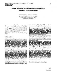
Figure 1. Variables defined in the GHT.

work with motion vectors in MPEG streams. However, since motion vectors are usually computed using a blockmatching technique, they are prone to be erroneous with respect to the real motion. 9, 11 This work presents a new technique to perform global motion estimation on MPEG compressed video, with application to video annotation. In fact, it is an evolution of a previous work where a feature extraction algorithm for video segmentation was stated.12 In that work a version of the well-known Hough Transform,13 known as Generalized Hough Transform14 (GHT), is used to perform feature extraction from MPEG compressed video streams. Then, a scene cut detection algorithm is stated. In this paper, the feature extraction technique is used to develop algorithms that allow the detection of pan, tilt, swing∗ and zoom effects. Here we assume that the possibility to distinguish between translation along the z-axis and zoom, as well as translation along the x and y axes and pan (rotation along y-axis) and tilt (rotation along x-axis) respectively depends on the scene content. Thus, it is assumed that the captured scene is flat concerning the depth along the z-axis, and so pan and tilt will be reported as camera translations. Motion information will allow further processing in order to infer semantic information from the video, or simply to detect certain motion effects. This paper is organized as follows. Section 2 gives an overview about the GHT. Section 3 describes the application of the GHT based feature extraction technique to global motion estimation. Experimental results are shown in Sect. 4. Finally, conclusions and some ideas about future work are stated in Sect. 5.

2. REVIEW OF THE GENERALIZED HOUGH TRANSFORM The Hough Transform13 was originally used to detect parametric shapes in binaries images. It is a very robust technique that can even be applied with missing or noisy data. Ballard16 generalized the Hough Transform to detect arbitrary shapes by computing a reference table used to calculate the rotation, scale and displacement of a template in an image. This technique had high memory and computational requirements. Thus, several improvements were proposed. One of the most interesting was proposed by Guil et al. 14 In that work, the detection process is split into three stages by uncoupling the rotation, scale and displacement calculation, achieving lower computational complexity. An evolution of this technique was presented in Ref. 17, where a complete description is stated. A little review of the process will be done. Let E be the edge points set in an image. The edge points of the image are characterized by the parameters (x, y, θ), where x and y are the coordinates in two dimensional space and θ is the angle of the gradient vector associated to this edge point. An angle, ξ, called difference angle is also defined. Its value indicates the positive difference between the angles of the edge points gradient vectors that will be paired. All the variables abovementioned are shown in Fig. 1.

∗ The basic camera operations, as defined in Ref. 15, are pan, tilt, swing, zoom and translation, where swing is the rotation along the z-axis.

From this description, three transformations will be defined. Let pi and pj be two edge points, (xi , yi , θi ) and (xj , yj , θj ) their associated information, and ξ the difference angle to pair points, transformation T can be written as follows: ½ (θi , αij ) θj − θi = ξ T (pi , pj ) = (1) 0 elsewhere µ ¶ yi − y j 6 αij = arctan θi , xi − x j that is, αij is the positive angle formed by the line that connects pi and pj and the gradient vector angle of the point pi . Transformation S uses a similar expression to that in Eq. 1 to calculate the distance between the two paired points. This transformation is defined as follows: ½ (θi , αij , dij ) θj − θi = ξ S(pi , pj ) = (2) 0 elsewhere q dij = (xi − xj )2 + (yi − yj )2 . Finally, transformation D uses an arbitrary reference point O and two vectors r~i and r~j : ½ (θi , αij , r~i , r~j ) θj − θi = ξ D(pi , pj ) = 0 elsewhere

(3)

r~k = O − pk , k = i, j. Transformation T can be used to compute the rotation angle β. The result of applying transformation T to the image is an image orientation table (IOT ) whose cells contain the pairings obtained. α and θ values are stored in rows and columns respectively. When a pairing with an αij and θj value is calculated, IOT [αij ][θj ] position is increased. Because different pairings might coincide with the same αij and θj values, the content of IOT [αij ][θj ] will indicate how many of them have these values. This transformation is also applied to the template to obtain a template orientation table (T OT ). α values are unaffected by rotation, scale and displacement, while θ is only affected by rotation. Then, if the template is included in the image, the T OT will be included in the IOT . If the template is rotated in the image, the T OT will be shifted circularly in the column direction in the IOT . Figure 2 shows the T OT of a rectangle, and the T OT of the same rectangle rotated 45 ◦ . To obtain the value of β a modified normalized cross correlation function is used. 18 A modified correlation process is needed because sampling errors, noise or small deformations can make the paired points spread in a small window around the ideal (α, θ) value. Thus, correlation should be carried out using points in the T OT and small windows in the IOT . The value of r that originate the maximum value of R(r) will indicate the rotation angle β. The expression of this modified correlation process is given below: P P T OT [α][θ − r] · W [IOT [α][θ]] R(r) = α θ (4) N IO · N TO sX X N IO = IOT [α][θ] · W [IOT [α][θ]] α

N TO =

θ

sX X α

W [F [i][j]] =

T OT [α][θ] · W [T OT [α][θ]]

θ

XX

F [i + w1 ][j + w2 ].

w1 w2

Transformation S is invariant to displacement and proportional to scale. This transformation is applied to the template to obtain a template scale table (T ST ) which contains the distances between the paired points in

360 α 0

θ

45º

360 α 0 360

θ

0

Figure 2. T OT of a rectangle.

the template. On the other side, transformation D is applied to the image to obtain an image displacement table (IDT ). The rotation angle β, computed in the previous step, is used to shift circularly the T ST . Then, cells in T ST and IDT with the same (α, θ) values are compared to obtain the scale factor s. The distance between every pair of points in IDT [α][θ] is computed and compared with all the distances in T ST [α][θ] to vote in a one-dimensional accumulator array. Maxima in this accumulator indicate possible scale values. A more evolved technique to calculate s is to use T ST and IDT to obtain two vectors, template distances histogram (T DH) and image distances histogram (IDH). These two vectors are the histograms of the distances of every pairing in both the template and the image respectively. T ST is shifted circularly using β. Then, non null cells in T ST and IDT with the same (α, θ) values are used to compute T DH and IDH respectively. Next, T DH is scaled for every scale value s within a predefined range, obtaining T DH s . Finally, a correlation process is performed between every T DHs and IDH. The correlation value is stored in S(s). The maximum value of S(s) will indicate the value of the scale factor s. The expression of the correlation process is similar to that one in Eq. 4. It is given below: P IDH[d] · W [T DHs [d]] (5) S(s) = d N IS · N TS sX N IS = IDH[d] · W [IDH[d]] d

N TS =

sX

T DHs [d] · W [T DHs [d]]

d

W [F [i]] =

X

F [i + w].

w

Finally, transformation D is applied to the template to obtain a template displacement table (T DT ). The rotation angle β is used to shift it circularly. Non null cells in T DT and IDT with the same (α, θ) values are compared. The reference vectors stored in T DT [α][θ] are scaled and applied to the coordinates of the paired points in IDT [α][θ] to vote in a bidimensional space. The maximum position in this space will indicate the situation d, in the image, of the reference point defined in the template shape. Figure 3 shows the segmentation of the method. The first stage computes the rotation β of the template in the image using only the information provided by T OT and IOT . β, along with T ST and IDT , are used in the second stage, where the scale factor s is computed. Finally, the third stage makes use of β, s, T DT and IDT to obtain the coordinates d in the image, of the reference point defined in the template. This method allows to use more than only one difference angle ξ. The extra information obtained with the usage of more than one difference angle can be useful to deal with special shapes, occlusions and/or noisy images.

Image D

T

IOT

IDT

T

d

Voting in a bidimensional space

TST

S

TOT

β, and displacement

s

Distance comparison and one-dimensional voting

Correlation restricted to row rotation

PSfrag replacements

s

β and scale factor

Rotation angle β

TDT

D

Template

Figure 3. Segmentation of the process.

3. ALGORITHMS FOR GLOBAL MOTION ESTIMATION Transformations T , S and D defined by the GHT allow the detection of arbitrary shapes in binaries images. Although it was originally designed to work with images, the application of the GHT to video processing has yielded interesting results when developing scene cut detection algorithms. 12 The way in which the GHT is applied to video processing is the following: Let us assume that template and image are two different frames from a video stream, fi and fj , where i + l = j and l is a small value so that fi and fj belong to the same shot. Thus, transformations T , S and D are applicable to fi and fj , so that rotation, scale and displacement values can be computed between them. The basis of the algorithm is to set a swing, zoom or displacement mark for every frame in the video stream where the appropriate kind of motion has been detected. It computes rotation, scale and displacement values along a n-frame window. The first frame in the window (f ) is compared to the next ones (f +1, f +2, . . . , f +n−1) obtaining n − 1 values of rotation (RV (0), . . . , RV (n − 1)), scale (SV (0), . . . , SV (n − 1)) and displacement (DV (0), . . . , DV (n − 1)). Further study of these values will allow to mark frame f as a swinging, zooming and/or displacing frame, according to rotation, scale and displacement values respectively. Finally, as a swing, zoom or displacement effect lasts for several frames, some of these frames may remain undetected. Thus, a process to properly mark these frames has to be carried out. Also, isolated detections lasting for less than a predefined number of frames should be removed. Next sections will describe these steps in more depth. Although this method is suitable to process uncompressed video sequences, full decompression of video and subsequent processing has two main drawbacks. On one hand, time is spent on performing the full decompression stage. On the other hand, the amount of data to be processed is considerably higher, increasing processing time. As we did in Ref. 12, we propose to work with the DC coefficients from the MPEG stream in order to obtain DC images as a subsampled representation of the full frame. Once the DC image has been computed from the MPEG stream, the aforementioned algorithm is applied. The process to obtain estimated values for all DC coefficients in every frame in the stream (type I, P or B) is stated in Ref. 19.

3.1. Swing detection To establish whether frame f has to be marked as a swinging frame or not, transformation T is applied to every frame in the window obtaining n orientation tables (OT0 , . . . , OTn−1 ). Remember that a n-frame window starting

Algorithm 1 Swing detection 1: rotCW ← 0 2: rotCCW ← 0 3: for i = 0 to n − 1 do 4: if RV (i) > 180 then 5: rotCW ← rotCW + 1 6: speedCW ← k360 − RV (i)k/(i + 1) 7: else if RV (i) ≤ 180 and RV (i) 6= 0 then 8: rotCCW ← rotCCW + 1 9: speedCCW ← RV (i)/(i + 1) 10: end if 11: end for 12: if rotCW > 0.75 ∗ n then 13: return (CW, speedCW ) 14: else if rotCCW > 0.75 ∗ n then 15: return (CCW, speedCCW ) 16: end if 17: return (NO, 0) at frame f is used. Application of Eq. 4 to each pair of tables ((OT0 , OT1 ), (OT0 , OT2 ), . . . , (OT0 , OTn−1 )) will generate n − 1 rotation values (RV (0), . . . , RV (n − 1)). Then, the process depicted in Alg. 1 is performed. The idea is to study the values in RV vector to conclude whether a swing effect is taking place or not, and, in the first case, to estimate the swing direction (clockwise or counterclockwise) as well as swing speed (in degrees per frame). Suppose that most of the rotation values in RV are 0. This clearly indicates that no swing effect has been detected. However, suppose that RV shows increasing (decreasing) values. This indicates that a counterclockwise (clockwise) swing effect is taking place. The magnitude of the values in RV will be useful to estimate swing speed. Lines 3 to 11 in Alg. 1 make a count of the number of rotation values that indicate a clockwise swing (rotCW ), as well as a counterclockwise swing (rotCCW ). Also, rotation speed is estimated in degrees per frame. Then, a swing effect is declared if at least 75% of the rotation values in RV point in the same direction (clockwise or counterclockwise). This is done in lines 12 to 17. Swing detection algorithm is carried out for every frame in the video sequence that is being analysed. It sets a swing mark for every frame belonging to a swing effect. However, depending on the conditions of the swing, it could fail for certain frames. Thus, a final stage to set swing marks for all the frames belonging to a swing effect that have not been marked in the previous stage is needed. Figure 4 shows a clockwise swing effect which lasts for 10 frames, from frame n to frame n + 9. Numbers under ROT CW label represent the speed of the rotation, in degrees per frame. However, frames n + 3, n + 6 and n + 7 have not been marked, while frame n + 5 has been incorrectly marked as a counterclockwise rotating frame. Interpolation mechanisms are used to correctly mark these frames as clockwise rotating frames and estimate the approximate rotation speed. This stage also performs the removal of isolated detections which last for less than a predefined number of frames. Frame n + k in Fig. 4 illustrates this situation.

3.2. Zoom detection Zoom detection is very similar to swing detection. However, transformation S is used instead of transformation T . Comparison of scale tables (ST ) using Eq. 5 will report scale factors that will be analysed in the same way as Alg. 1 in order to set a zoom in or a zoom out mark for the current frame. A final stage to mark missed detections within a detected zoom effect, interpolate estimated zoom speed and remove isolated detections is also needed.

Frame

n ROT CW 1.00

n+1

n+2

ROT CW 1.50

ROT CW 2.00

n+3

n+4

n+5

ROT CW 3.00

ROT CCW 1.50

n+6

n ROT CW 1.00

n+8

n+9

n+k

ROT CW 2.00

ROT CW 1.00

ROT CW 1.50

Algorithm to fill in holes and remove isolated detections

Missed detections added

Frame

n+7

False detections removed

n+1

n+2

n+3

n+4

n+5

n+6

n+7

n+8

n+9

ROT CW 1.50

ROT CW 2.00

ROT CW 2.50

ROT CW 3.00

ROT CW 2.75

ROT CW 2.50

ROT CW 2.25

ROT CW 2.00

ROT CW 1.00

n+k

Figure 4. Operation of the algorithm to fill in holes and remove isolated detections.

3.3. Displacement detection Once again, the algorithm to detect camera displacements is similar to swing and zoom detection. In this case, transformation D is used to obtain n−1 displacement values (DV (0), . . . , DV (n−1)), all of which will be analysed using Alg. 2 in order to estimate displacement angle αd and relative speed vd . Pan and tilt displacement in pixels can be directly obtained from αd and vd by applying the following expressions: Pan displacement (pixels)

=

8 · vd · cos αd

(6)

Tilt displacement (pixels)

=

8 · vd · sin αd

(7)

The expressions above are multiplied by 8 because DC images instead of full frames are used to perform displacement calculation. Dimensions of DC images are eight times smaller in each dimension than those in full frames. To declare a displacement for frame f and estimate displacement angle and speed, Alg. 2 is used. The idea is similar to that one used in Alg. 1. However, the problem is a little more complicated as there are not only two directions (clockwise or counterclockwise) but many of them. Suppose that points in DV are aligned with a vector. Direction of the vector is 45◦ . This indicates a mixed pan-right, tilt-up effect. Also, modulus of the vector will indicate relative displacement speed. Lines 2 to 16 in Alg. 2 show the process to fill in an orientation histogram h using points in DV . Each bin in h stores three values: the number of points which orientation is within the range defined by that bin (h(i).n), the mean orientation of those points (h(i).angle), and finally the mean relative speed of the displacement in that direction (h(i).speed). Methods PointDirection and HistogramBin are used to calculate the histogram bin associated with every point analysed. CalcDisplacementSpeed computes the relative displacement speed for that point. Once that histogram h has been filled in, line 17 computes the highest bin in h, that is, the bin which stores the highest number of points. Then, a displacement effect is declared if at least 50% of the displacement values in DV are in the highest bin in h (lines 18 to 21). Again, a process similar to that one depicted in Fig. 4 is needed to correctly mark undetected frames within a displacement effect and remove isolated detections which last for less than a predefined number of frames. Interpolation mechanisms are used to estimate the correct displacement angle as well as relative speed.

4. EXPERIMENTAL RESULTS This section evaluates the performance of the proposed global motion estimation algorithm working with MPEG compressed video. Instead of using several videos to study different effects, this work mainly uses a video sequence that contains several occurrences of each effect to be detected. This sequence, which was recorded using a camcorder, has 13500 frames and includes 21 swings, 38 zooms and 42 displacements. A sequence with

Algorithm 2 Displacement detection 1: h ← CreateEmptyHistogram() 2: for i = 0 to n − 1 do 3: if DV (i) 6= (0, 0) then 4: d ← PointDirection(DV (i)) 5: bin ← HistogramBin(d) 6: s ← CalcDisplacementSpeed(DV (i))/(i + 1) 7: if h(bin).n = 0 then 8: h(bin).angle ← d 9: h(bin).speed ← s 10: else 11: h(bin).angle ← AngleMean(h(bin).angle, d) 12: h(bin).speed ← (h(bin).speed + s)/2 13: end if 14: h(bin).n ← h(bin).n + 1 15: end if 16: end for 17: b ← HighestBin(h) 18: if h(b).n > 0.5 ∗ n then 19: return (h(b).angle, h(b).speed) 20: end if 21: return (NO, 0) such characteristics also allows the study of how the presence of certain effects affects the detection of others. For example, certain zoom effects cause false displacement detections. Two more sequences have been used in order to study displacement effects in more depth. One of these sequences has been specifically recorded to include a pan-right which gradually turns into a tilt-up displacement. The other sequence is the well-known coast guard sequence, often used to study global motion algorithms. All the sequences are in SIF (352 × 240) format. The hardware configuration used to run the tests consists of an AMD Athlon K7, 1 GHz, 256 MB RAM, running Linux 2.2.16. The algorithms have been codified using the GNU g++ compiler version 2.95.2. Different performance statistics have been stated in the literature. This work considers correct and missed detections as well as recall and precision statistics for swing, zoom and displacement effects. On one hand, a detection is said to be correct if at least 50% of the frames belonging to the effect have been correctly marked. On the other hand, accuracy of the detections as well as false detections are considered in recall and precision figures. Recall defines the percentage of correctly detected frames in relation to the overall frames of a certain effect in the video. Precision defines the percentage of correctly detected frames in relation to the overall frames of a certain effect detected by the algorithm. Mathematical expressions for these parameters are given below: Recall (%)

=

Precision (%)

=

c c+m c 100 · c+f 100 ·

(8) (9)

where c is the number of correctly detected frames, m is the number of missed frames, and f is the number of falsely detected frames. Note that recall and precision statistics rely on the number of correctly or falsely detected frames, or missed frames. However, correct and missed figures refer not to frames but to effects, composed of several frames. Table 1 shows the experimental results of the proposed detection method applied to the first of the test sequences. A 10 frame window as well as 2 pairing angles, 180◦ and 135◦ have been used. Proposed method yields very good results for swing and displacement detections and interesting ones for zoom detections. 100% of the swing effects are correctly detected (21 out of 21). Also, 85% of recall and 95% of precision show that detections are very accurate. Figure 5 shows cumulative rotation angle for a 90 ◦ clockwise swing effect that

Motion effect Swing Zoom Displacement

Correct 21 32 41

Missed 0 6 1

Recall 85% 75% 94%

Precision 95% 83% 90%

Table 1. Experimental results of the proposed global motion estimation algorithm.

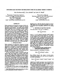
takes place between frames 1219 and 1293 in analysed video sequence. As it is shown in Fig. 5, accumulated rotation angle at frame 1293 is 92.05◦ , which evidences the accuracy of the detection. Even better figures are reported when displacement effects are considered. Most of false displacements reported are due to zoom effects. Test have revealed that zoom detection is a little more complicated. However, 84% of the zoom effects are correctly detected (32 out of 38). False zoom detections are often caused by displacements, resulting in short zoom detections lasting for less than 15 frames. Time spent on performing motion estimation is about 1.7 seconds per frame, using the hardware configuration stated before. Figures 6 and 7 display functions estimated directly from the data reported by the proposed algorithm for displacement effects. Figure 6 shows displacement angle as well as pan/tilt rate for a sequence including a pan-right which gradually turns into a tilt-up displacement. Figure 6(a) clearly shows that a pan-right (0 ◦ ) displacement takes place between frames 75 and 135. Also, Fig. 6(b) shows an increasing pan rate while tilt rate holds a value of 0 pixels per frame. From frame 135 until 180, the displacement angle gradually tends to 90◦ . Pan rate decreases while tilt rate rises. From frame 180, displacement angle maintains a value of 90 ◦ , which indicates a pure tilt-up displacement. Also, pan rate is 0 during a tilt movement. Similarly, Fig. 7 shows displacement angle and pan/tilt rate for sequence coast guard. This sequence has two pan movements, pan-left between frames 0 and 65 and pan-right between frames 83-300, as well as a tilt-up between frames 65-75. Figure 7(a) shows displacement angles for the three different displacement effects detected. Also, pan and tilt rates are shown in Fig. 7(b). Pan rate is negative in pan-left effects, and positive in pan-right effects. Tilt rate holds a value of 0 pixels per frame except for the tilt effect, where it reaches values of about 5 pixels per frame. To obtain the results in Fig. 7 some parameters of the algorithm had to be adjusted. During the pan-left displacement a coast guard ship is moving to the right. Due to the dimensions of the object the algorithm is unable to estimate the global motion in some frames. Thus, parameter 0.5 in line 18 of Alg. 2 has been reduced to 0.4. Also, as the tilt-up motion is so fast and short, a 8 frames window instead of 10 has been used.

5. CONCLUSIONS This work presents a new global motion estimation algorithm based on the GHT. This technique allows the comparison of two images in order to obtain rotation, scale and displacement parameters. GHT algorithm has 100 90

Cumulative Rotation Angle (degrees)

80 70 60 50 40 30 20 10 0 1220 1225 1230 1235 1240 1245 1250 1255 1260 1265 1270 1275 1280 1285 1290 Frame

Figure 5. Cumulative rotation angle for a 90◦ clockwise swing effect.

been applied to video sequences in order to perform global motion estimation. Thus, this work presents an algorithm able to detect swing, zoom and displacement effects in video sequences. Moreover, the proposed method works with MPEG compressed video. As opposed to many other works, our proposal does not rely on motion vectors from the MPEG stream to perform motion estimation, as they are prone to be erroneous with respect to the real motion. Also, motion vectors accuracy depends on the quality of the MPEG compressor. Hence, this work proposes to work with DC images, avoiding the use of MPEG motion vectors. Obtained results show that the proposed algorithm performs quite well when detecting swing and camera displacement effects. Existing effects are successfully detected. Also, start and final frames estimation is often very accurate. Zoom detection is not so precise. However, very interesting results have been obtained although start and final frames are sometimes inexact. Future work will concentrate on the development of algorithms to infer semantic information from video sequences. The proposed global motion estimation algorithm will be very helpful in such task. Algorithms to detect gradual transitions such as dissolves, fades, etc. will also be developed.

REFERENCES 1. Y.-P. Tan, D. D. Saur, S. R. Kulkarni, and P. J. Ramadge, “Rapid estimation of camera motion from compressed video with application to video annotation,” IEEE Trans. on Circuits and Systems for Video Technology 10, pp. 133–146, February 2000. 2. A. Kokaram and P. Delacourt, “A new global motion estimation algorithm and its application to retrieval in sports events,” in Proc. IEEE Workshop on Multimedia Signal Processing (MMSP01), (Cannes, France), October 2001. 3. D. Adolph and R. Buschmann, “1.15 mbit/s coding of video signals including global motion compensation,” Signal Processing: Image Communications 3(2–3), pp. 259–274, 1990. 4. Y. T. Tse and R. L. Baker, “Global zoom/pan estimation and compensation for video compression,” in Proc. IEEE Proceedings of International Conference on Acoustics, Speech and Signal Processing (ICASSP91), pp. 2725–2728, (Toronto, Ontario, Canada), May 1991. 5. H. Jozawa, K. Kamikura, A. Sagata, H. Kotera, and H. Wanatabe, “Two stage motion compensation using adaptative global mc and local affine mc,” IEEE Trans. on Circuits and Systems for Video Technology 7, pp. 75–85, February 1997. 6. S. Wu and J. Kittler, “A differential method for simultaneously estimation of rotation, change of scale and translation,” Signal Processing: Image Communications 2(1), pp. 69–80, 1990. 7. F. Moscheni, F. Dufaux, and M. Kunt, “A new two-stage global/local motion estimation based on a background/foreground segmentation,” in Proc. IEEE Proceedings of International Conference on Acoustics, Speech and Signal Processing (ICASSP95), pp. 2261–2264, (Detroit, MI, USA), May 1995. 8. M. Etoh and T. Ankei, “Parametrized block correlation–2d parametric motion estimation for global motion compensation and video mosaicing,” July 1997. IECE TR PRMU97. 9. J. Heuer and A. Kaup, “Global motion estimation in image sequences using robust motion vector field segmentation,” in Proc. ACM Multimedia 99, pp. 261–264, (Orlando, FL, USA), October 1999. 10. H. Zhang, C. Low, and S. Smoliar, “Video parsing and browsing using compressed data,” Multimedia Tools and Applications 1, pp. 89–111, March 1995. 11. H. Wang, A. Divakaran, A. Vetro, S.-F. Chang, and H. Sun, “Survey on compressed-domain features used in video/audio indexing and analysis,” tech. rep., Dept. Electrical Engineering, Columbia University, NY, USA, 2000. 12. E. S´aez, J. M. Gonz´alez, J. M. Palomares, J. I. Benavides, and N. Guil, “New edge-based feature extraction algorithm for video segmentation,” in IS&T/SPIE Symposium Proceedings, Image and Video Communications and Processing, 5022, (Santa Clara, CA, USA), January 2003. 13. P. Hough, “A method and means for recognizing complex patterns,” 1962. U.S. Patent No. 3,069,654. 14. N. Guil and E. Zapata, “A fast generalized hough transform,” in Proc. European Robotic and Systems Conference, pp. 498–510, (M´alaga, Spain), 1994.

15. Y. Tan, S. Kulkarni, and P. Ramadge, “A new method for camera motion parameter estimation,” in Proc. IEEE International Conference on Image Processing, 1, pp. 406–409, 1995. 16. D. Ballard, “Generalizing the hough transform to detect arbitrary shapes,” Pattern Recognition 13(2), pp. 111–122, 1981. 17. N. Guil, J. Gonz´alez, and E. Zapata, “Bidimensional shape detection using an invariant approach,” Pattern Recognition 32, pp. 1025–1038, 1999. 18. J. Gonz´alez, N. Guil, and E. Zapata, “Detection of bidimensional shapes under global deformations,” in Proc. X European Signal Processing Conference (EUSIPCO 2000), (Tampere, Finland), September 2000. 19. B. Yeo and B. Liu, “Rapid scene analysis on compressed videos,” IEEE Trans. on Circuits and Systems for Video Technology 5(6), pp. 533–544, 1995.

105

8

90

7

Pan Rate Tilt Rate

6 Displacement Speed (pixels/frame)

Displacement Angle (degrees)

75

60

45

30

15

5

4

3

2

1

0

0

-15

-1 75

90

105

120

135

150

165 180 Frame

195

210

225

240

255

270

75

90

105

120

(a) Displacement angle

135

150

165 180 Frame

195

210

225

240

255

270

(b) Pan/tilt rate

Figure 6. Displacement angle and pan/tilt rate for a sequence that includes a pan-right displacement which gradually turns into a tilt-up displacement.

195

6 Pan Rate Tilt Rate

180

5

165 4 Displacement Speed (pixels/frame)

Displacement Angle (degrees)

150 135 120 105 90 75 60 45 30

3 2 1 0 -1 -2

15 -3

0 -15

-4 0

15

30

45

60

75

90 105 120 135 150 165 180 195 210 225 240 255 270 285 Frame

(a) Displacement angle

0

15

30

45

60

75

90 105 120 135 150 165 180 195 210 225 240 255 270 285 Frame

(b) Pan/tilt rate

Figure 7. Displacement angle and pan/tilt rate for coast guard sequence.