Motion Estimation for Video Coding Standards - Springer Link

P1: VTL/ASH

P2: VTL

Journal of VLSI Signal Processing

KL494-03-Hang

October 9, 1997

13:21

Journal of VLSI Signal Processing 17, 113–136 (1997) c 1997 Kluwer Academic Publishers. Manufactured in The Netherlands. °

Motion Estimation for Video Coding Standards HSUEH-MING HANG, YUNG-MING CHOU AND SHEU-CHIH CHENG Department of Electronics Engineering and Microelectronics and Information Systems Research Center, National Chiao Tung University, 1001 Ta-Hsueh Road Hsinchu 300, Taiwan, R.O.C.

Abstract. Motion-compensated estimation is an effective means in reducing the interframe correlation for image sequence coding. Therefore, it is adopted by the international video coding standards, ITU H.261, H.263, ISO MPEG-1 and MPEG-2. This paper provides a comprehensive survey of the motion estimation techniques that are pertinent to video coding standards. There are three popular groups of motion estimation methods: i) block matching methods, ii) differential (gradient) methods, and iii) Fourier methods. However, not all of them are suitable for the block-based motion compensation structure specified by the aforementioned standards. Our focus in this paper is to review those techniques that would fit into the standards. In addition to the basic operations of these techniques, issues discussed are their extensions, their performance limit, their relationships with each other, and the other advantages or disadvantages of these methods. At the end, an example of evaluating block matching algorithms from a system-level VLSI design viewpoint is provided.

1.

Introduction

Motion-compensated estimation is an effective means in reducing the interframe correlation for image sequence coding. Therefore, it is adopted by international video coding standards: ITU H.261 [1], H.263 [2], ISO MPEG-1 [3], and ISO MPEG-2 [4]. This paper provides a comprehensive survey of the motion estimation techniques that are pertinent to video coding standards. It may worth mentioning that although motion estimation is also used in many other disciplines such as computer vision, target tracking, and industrial monitoring, the techniques developed particularly for image coding are different in some respects. The goal of image compression is to reduce the total transmission bit rate for reconstructing images at the receiver. Hence, the motion information should occupy only a small amount of the transmission bandwidth additional to the picture contents information. As long as the motion parameters we obtain can effectively reduce the total bit rate, these parameters need not be the true

motion parameters. Besides, the reconstructed images at the receiving end are often distorted. Therefore, if the reconstructed images are used for estimating motion information, a rather strong noise component cannot be ignored. An interesting point in studying the motion estimation techniques for standards is that the current video standards specify only the decoders. Assuming motion displacement information (motion vectors) are generated by the encoder and transmitted to the decoder, the decoder only performs the motion compensation operation—patch the to-be-reconstructed picture using the known (already decoded) picture(s). The encoder, which performs the motion estimation operation, is not explicitly specified in the standards. Hence, it is possible to use different motion estimation techniques to produce standards-compatible motion information. At the decoder, other than the sources of coded pictures that can be used for motion compensation, essentially the same block-based motion compensation operation is used by all the popular video standards, H.261, H.263, MPEG-1, and MPEG-2. This specific decoder motion

P1: VTL/ASH

P2: VTL


114

KL494-03-Hang

October 9, 1997

13:21

Hang, Chou and Cheng

compensation structure poses certain constraints on the standard-compatible motion estimators at the encoder; however, a significant amount of flexibility still exists in choosing and designing a motion estimation scheme for a standard coder. Motion estimation techniques for image coding have been explored by many researchers over the past 25 years [5–7]. These techniques can be classified, roughly, into three groups: i) block matching methods, ii) differential (gradient) methods, and iii) Fourier methods [8]. However, not all of them are suitable for the block-based motion compensation structure adopted by the aforementioned standards. Our focus in this paper is to review those techniques that would fit into the standards. This paper is organized as follows. In Section 2, we first give a general introduction to the motion estimation problem for image sequence coding. Also included in this section is a brief discussion on the performance limit of motion compensation in bit rate reduction. Block matching technique is very popular and is generally considered robust and effective for image coding. Section 3 describes the basic block matching scheme and the fast search algorithms that reduce computational complexity. Section 4 describes another popular approach of estimating motion vectors; it is often called the differential method or the spatiotemporal gradient method. Although the original form of this technique was not invented for block motion compensation, some of its variations can produce the motion information format defined by the standards. The third group of motion estimation methods, the Fourier method, is described in Section 5. This group of methods are not as popular as the previous two groups. But they are block-based and thus can fit into the video standards easily. This approach can also provide us insights in understanding the underlying principle of motion estimation algorithms and can thus be used as a tool to analyze the limits of motion estimation. Section 6 discusses the impact of different block matching algorithms on VLSI design. A fast algorithm that merely reduces arithmetic operations may not have the best overall VLSI performance. This paper ends with a brief conclusion section. 2.

period of time. Motion estimation is the operation that estimates the motion parameters of moving objects in an image sequence. Frequently, the motion parameters we look for are the displacement vectors of moving pels between two picture frames. On the other hand, motion compensation is the operation of predicting a picture, or portion thereof, based on displaced pels of a previously transmitted frame in an image sequence.

2.1.

Motion Estimation

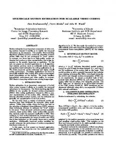
In the physical world, objects are moving in the 4-dimensional (4-D) spatio-temporal domain—three spatial coordinates and one temporal coordinate. However, images taken by a single camera are the projections of these 3-D spatial objects onto the 2-D image plane as illustrated in Fig. 1. A 3-D point P(x, y, z) is thus represented by a 2-D point P 0 (X, Y ) on the image plane. Hence, if pels on the image plane (the outputs from an ordinary camera) are the only data we can collect, the information we have is a 3-D cube— two spatial coordinates and one temporal coordinate. The goal of motion estimation is to extract the motion information of objects (pels) from this 3-D spatiotemporal cube. In reality, video taken by an ordinary camera is first sampled along the temporal axis. Typically, the temporal sampling rate (frame rate) is 24, 25, or 29.97 frames (pictures) per second. Spatially, every frame is sampled vertically into a number of horizontal lines. For example, the active portion of an NTSC TV frame (i.e., the portion containing the image) has about 483 lines. In the case of the digitized images

Motion Estimation and Compensation

In the rest of this paper we assume that the image sequences under consideration contain moving objects whose shape does not change much, at least over a short

Figure 1.

Perspective projection geometry of image formulation.

P1: VTL/ASH

P2: VTL


KL494-03-Hang

October 9, 1997

13:21

Motion Estimation for Video Coding Standards

that are almost exclusively used in this paper, a line is sampled into a number of pels. According to the CCIR 601 standard, the active portion of an NTSC TV line consists of 720 pels. Practically, to reduce computation and storage complexity, motion parameters of objects in a picture are estimated based on two or three nearby frames. Most of the motion estimation algorithms assume the following conditions: i) objects are rigid bodies; hence, object deformation can be neglected for at least a few nearby frames; ii) objects move only in translational movement for, at least, a few frames; iii) illumination is spatially and temporally uniform; hence, the observed object intensities are unchanged under movement; iv) occlusion of one object by another and uncovered background are neglected [6]. Often, practical motion estimation algorithms can tolerate a small amount of inexact matches to these assumptions. Specifically, several algorithms have been invented that somewhat relieve some of these conditions. The motion estimation problem, in fact, consists of two related sub-problems: i) identify the moving object boundaries, so-called motion segmentation, and ii) estimate the motion parameters of each moving object, so-called motion estimation in strict sense. In our use, a moving object is a group of contiguous pels that share the same set of motion parameters. This definition does not necessarily match the ordinary meaning of object. For example, in a videophone scene, the still background may include wall, bookshelf, decorations, etc. As long as these items are stationary (sharing the same zero motion vector), they can be considered as a single object in the context of motion estimation and compensation. The smallest object may contain only a single pel. In the case of pel-recursive estimation (described in Section 4), it appears that we can calculate the motion vector for every pel; however, either a minimum set of 2 pels of data or additional constraint(s) has to be used in the process of estimating the 2-D motion vector. One difficulty we encounter in using small objects (or evaluation windows) is the ambiguity problem—similar objects (image patterns) may appear at multiple locations inside a picture and may lead to incorrect displacement vectors. Also, statistically, estimates based on a small set of data are more vulnerable to random noise than those based on a larger set of data. Alternatively, if a large number of pels are treated as a single unit for estimating their motion parameters, we must first know precisely the moving object boundaries. Otherwise,

115

we encounter the accuracy problem—pels inside an object or evaluation window do not share the same motion parameters and, therefore, the estimated motion parameters are not accurate for some or all pels in it. On the other hand, the criterion of grouping pels into moving objects, no matter which scheme is in use, must be consistent with the motion information of every pel. Hence, we are running into the chicken and egg dilemma: accurate motion information for every pel is necessary for precise moving object segmentation, and precise object boundaries are necessary for computing accurate motion parameters. There exist practical solutions to circumvent the aforementioned motion segmentation and motion estimation dilemma. One solution is partitioning images into regular, nonoverlapped blocks; assuming that moving objects can be approximated reasonably well by regular shaped blocks. Then, a single displacement vector is estimated for the entire image block under the assumption that all the pels in the block share the same displacement vector. This assumption may not always be true because an image block may contain more than one moving object. In image sequence coding, however, prediction errors due to imperfect motion compensation are coded and transmitted. Hence, because of its simplicity and small overhead this block-based motion estimation/compensation method is widely adopted in real video coding systems. The other extreme is the pel-based method that treats every single pel as the basic motion estimation unit. Its motion vector is computed over a small neighborhood surrounding the evaluated pel. No explicit object boundaries are assumed in this approach; however, it suffers from the aforementioned ambiguity problem and, in addition, because of the small data size it suffers from the noise problem. Therefore, the block-based approach is adopted by the video standards partially, at least, due to its robustness. 2.2.

Motion-Compensated Coding and Standards

The explicit use of motion compensation to improve video compression efficiency can be dated back to the late 1960s, a patent filed by Haskell and Limb [9] and a paper by Rocca presented at Picture Coding Symposium [10], both in the year of 1969. A number of coding structures using motion-compensated prediction have since then been proposed [5, 6, 11–14]. Although detailed implementation of motion-compensated systems varied significantly over the past 25

P1: VTL/ASH

P2: VTL


116

Figure 2.

KL494-03-Hang

October 9, 1997

13:21


A general motion-compensated coding structure.

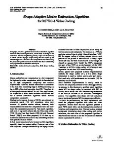
years, the general concept remains unchanged. Haskell and Limb stated in [9]: In an encoding system for use with video signals, the velocity of a subject between two frames is estimated and used to predict the location of the subject in a succeeding frame. Differential encoding between this prediction and the actual succeeding frame are used to update the prediction at the receiver. As only the velocity and the updating difference information need be transmitted, this provides a reduction in the communication channel capacity required for video transmission. The general structure of a motion-compensated codec is depicted in Fig. 2. For the moving areas of an image, there are roughly three processing stages at the encoder: i) motion parameter estimation, ii) moving pels prediction (motion compensation), and iii) prediction-errors/originalpels compression. Only two stages are needed at the decoder: i) prediction-errors/original-pels decompression, and ii) motion compensation. In these processes, the motion compensators at the encoder and at the decoder are similar. They often consist of two operations: i) access the previous-frame image data according to the estimated displacement vectors, and ii) construct the predicted pels by passing the previous-frame image through the prediction filter. The data compression and decompression processes are inverse operations of each other. They typically include the following elements: discrete transform, coefficient selection/quantization, and variable-word-length coding. The decoder defined by the video standards is very similar to the one shown in Fig. 2. Only one motion-

Figure 3.

Block motion estimation and compensation.

compensation mode is available in H.261 [1]. It uses the previously decoded frame to predict the current (tobe-coded) frame. The current frame is partitioned into 16 × 16 blocks. Each block is predicted by a shifted copy of the previous frame image block as shown in Fig. 3. There are three motion compensation modes in MPEG-1 and MPEG-2 [3, 4]. The so-called B-picture (or bi-directional picture) in MPEG-1 can use either the coded picture located before the current picture, the coded picture located after the current one, or both of them for prediction. In the case of using “both” pictures, the prediction of the current image block is the average of two reference image blocks, one from the past picture and the other from the future, as illustrated by Fig. 4. The same three prediction modes are also used by MPEG-2. In addition, a picture frame in MPEG-2 may contain two interleaved fields. Therefore, an image block may contain lines from either one field or both fields. To take the advantages of field and frame temporal correlation, MPEG-2 allows several combinations of using either fields or frames in

P1: VTL/ASH

P2: VTL


KL494-03-Hang

October 9, 1997

13:21


117

computation. A number of papers have been published since then improving or extending their method. There have gone roughly towards two directions. One direction was to reduce the computational load in calculating the motion vectors; the other was to increase the motion vector accuracy. The block matching motion estimation algorithms are used most often in today’s standard compatible video encoder.

Figure 4.

Figure 5.

MPEG-1 motion compensation modes.

MPEG-1 encoding order.

motion compensation. However, the techniques used at the encoder to estimate the motion vectors for all the above cases are similar. Before describing various motion estimation techniques, one remark we like to add here is the encoding order in MPEG standards. One may wander how we could access both the past and the future pictures in MPEG motion compensation. In a typical MPEG coded sequence, the encoding order looks like the one shown in Fig. 5. In this particular example, frame 1 is first coded without motion compensation. Then, frame 4 (not frame 2) is coded using frame 1 as reference. Afterward, in encoding frames 2 and 3, both frames 1 and 4 can be used as references. This arrangement has advantages in compression efficiency. Detailed description can be found in the standards document [3, 4]. 3.

Block Matching Method

Jain and Jain [15] suggested an interframe coding structure using the block matching motion estimation method and proposed a fast search algorithm to reduce

3.1.

Basic Concept

Block matching is a correlation technique that searches for the best match between the current image block and candidates in a confined area of the previous frame. Figure 3 illustrates the basic operation of this method. In a typical use of this method, images are partitioned into nonoverlapped rectangular blocks. Each block is viewed as an independent object and it is assumed that the motion of pels within the same block is uniform. The block matching method is essentially an object recognition approach. The displacement (motion) vector is the by-product when the new location of the object (block) is identified. The size of the block affects the performance of motion estimation. Small block sizes afford good approximation to the natural object boundaries; they also provide good approximation to real motion, which is now approximated by piecewise translational movement. However, small block sizes produce a large amount of raw motion information, which increases the number of transmission bits or the required data compression complexity to condense this motion information. From the performance viewpoint, small blocks also suffer from the object (block) ambiguity problem and the random noise problem. Large blocks, on the other hand, may produce less accurate motion vectors since a large block may likely contain pels moving at different speeds and directions. For typical images used for entertainment and teleconferencing, their picture sizes range from 240 lines by 352 pels to 1080 lines by 1920 pels (HDTV). Block sizes of 8 × 8 or 16 × 16 are generally considered adequate for these applications. The international video transmission standards, H.261, MPEG-1, and MPEG-2, all adopt the block size of 16 × 16. The basic operation of block matching is picking up a candidate block and calculating the matching function (usually a nonnegative function of the intensity differences) between the candidate and the current block. This operation is repeated until all the candidates have run through and then the best matched candidate is

P1: VTL/ASH

P2: VTL


118

KL494-03-Hang

October 9, 1997

13:21


on the computational complexity and the displacement vector accuracy. Let (d1 , d2 ) represent a motion vector candidate inside the search region and f (n 1 , n 2 , t) be the digitized image intensity at the integer-valued 2-D image coordinate (n 1 , n 2 ) of the tth frame. Several popular matching functions that appear frequently in the literature are as follows. 1. Normalized cross-correlation function (NCF): NCF(d1 , d2 ) =

[

PP

f (n 1 , n 2 , t) f (n 1 − d1 , n 2 − d2 , t − 1) PP 2 1/2 P P 2 1/2 f (n 1 , n 2 , t)] [ f (n 1 − d1 , n 2 − d2 , t − 1)]

2. Mean squared error (MSE): Figure 6.

Search region in block matching.

1 −1 N 2 −1 X 1 NX [ f (n 1 , n 2 , t) N1 N2 n 1 =0 n 2 =0

MSE(d1 , d2 ) = identified. The location of the best matched candidate becomes the estimated displacement vector. Several parameters are involved in the searching process: i) the number of candidate blocks, search points, ii) the matching function, and iii) the search order of candidates. All of them could have an impact on the final result. We often first decide on the maximum range of motion vectors. This motion vector range, search range, is chosen either by experiment or due to hardware constraints. Assume that the size of the image block is N1 × N2 and that the maximum horizontal and vertical displacements are less than dmax x and dmax y , respectively. For the moment, we consider only integer-valued motion vectors. Except for the blocks on the picture boundaries, the size of the search region SR is (N1 + 2dmax x )(N2 + 2dmax y ), and therefore, the number of possible search points equals to (2dmax x + 1)(2dmax y + 1), as shown by Fig. 6. The exhaustive search calculates the matching function of every candidate in the search region. Its computational load is thus proportional to the product of dmax x and dmax y . When the search range becomes fairly large, in the cases of large picture sizes or bi-directional coding (e.g., MPEG), both the computational complexity and the data input/output bandwidth grow very rapidly. 3.2.

Matching Function

It is necessary to choose a proper matching function in the process of searching for the optimal point. The selection of the matching function has a direct impact

− f (n 1 − d1 , n 2 − d2 , t − 1)]2 3. Mean absolute difference (MAD): MAD(d1 , d2 ) =

1 −1 N 2 −1 X 1 NX | f (n 1 , n 2 , t) N1 N2 n 1 =0 n 2 =0

− f (n 1 − d1 , n 2 − d2 , t − 1)| 4. Number of thresholded differences (NTD) [16]: NTD(d1 , d2 ) =

NX 1 − 1 NX 2 −1

N ( f (n 1 , n 2 , t),

n 1 =0 n 2 =0

f (n 1 − d1 , n 2 − d2 , t − 1)), where ½ N (α, β) =

1 if |α − β| > T0 0 if |α − β| ≤ T0

is the counting function with threshold T0 . To estimate the motion vector, we normally maximize the value of NCF or minimize the values of the other three functions. In detection theory, if the total noise, a combination of coding error and the other factors violating our motion assumptions, can be modeled as white Gaussian, then, NCF is the optimal matching criterion. However, the white Gaussian noise assumption is not completely valid for real images. In addition, because N1 N2 multiplications are needed for every candidate vector, the computational requirement

P1: VTL/ASH

P2: VTL


KL494-03-Hang

October 9, 1997

13:21


119

of NCF is considered to be enormous. The basic operation of the other three matching functions is subtraction, which is usually much easier to implement. Hence, they are regarded as more practical, and they perform almost equally well on real images. Notably NTD can be adjusted to match the subjective thresholding characteristics of the human visual system. However, its motion estimation performance is less favorable if the threshold value is not properly tuned for pictures and coding parameters. Overall, MAD has the advantages of good performance and relatively simple hardware structure—its absolute value operator versus the square operator in MSE, it becomes the most popular choice in designing practical image coding systems. 3.3.

Fast Search Algorithms

An exhaustive search examines every search point inside the search region and thus gives the best possible match; however, a large amount of computation is required. Several fast algorithms have thus been invented to save computation at the price of slightly impaired performance. The basic principle behind these fast algorithms is breaking up the search process into a few sequential steps and choosing the next-step search direction based on the current-step result. At each step, only a small number of search points are calculated. Therefore, the total number of search points is significantly reduced. However, because the steps are performed in sequential order, an incorrect initial search direction may lead to a less favorable result. Also, the sequential search order poses a constraint on the available parallel processing structures. Normally, a fast search algorithm starts with a rough search, computing a set of scattered search points. The distance between two nearby search points is called (search) step size. After the current step is completed, it then moves to the most promising search point and does another search with probably a smaller step size. This procedure is repeated until it cannot move further and the (local) optimum point is reached. If the matching function is monotonic along any direction away from the optimal point, a well-designed fast algorithm can then be guaranteed to converge to the global optimal point [15, 17]. But in reality the image signal is not a simple Markov process and it contains coding and measurement noises; therefore, the monotonic matching function assumption is often not valid and consequently fast search algorithms are often suboptimal.

Figure 7.

Illustration of 2D-log search procedure.

The first fast search block-matching algorithm is the 2D-log search scheme proposed by Jain and Jain [15]. It is an extension of the 1-D binary logarithm search. The searching procedure is illustrated by the example in Fig. 7. It starts from the center of the search region—the zero displacement. Each step consists of calculating five search points as shown in Fig. 7. One of them is the center of a diamond-shaped search area and the other four points are on the boundaries of the search area, n pels (step size) away from the center. This step size is reduced to half of its current value if the best match is located at the center or located on the border of the maximum search region. Otherwise, the search step size remains the same. The search area in the next step is centered at the best matching point as a result of the current step. When the step size is reduced to 1, we reach the final step. Nine search points in the 3 × 3 area surrounding the last best matching point are compared. The location of the best match determines the motion vector. Assuming the maximum search range is dmax ≥ 2 in both horizontal and vertical directions, the initial step size n would be equal to max(2, 2m−1 ), where m = blog2 dmax c and bzc denotes the largest integer less than or equal to z. For the example shown in Fig. 7 (dmax = 7), 6 steps and 22 calculated search points are required to reach the final destination at (3, 7). This total computational cost is much smaller than the exhaustive search that requires 225 search points in this case.

P1: VTL/ASH

P2: VTL


120

Figure 8.

KL494-03-Hang

October 9, 1997

13:21


Illustration of three step search procedure.

Another popular fast search algorithm is the socalled three step search proposed by Koga et al. [18] In their example and the example given in Fig. 8, the search starts with a step size equal to or slightly larger than half of the maximum search range. In each step, nine search points are compared. They consists of the central point of the square search area and eight search points located on the search area boundaries as shown in Fig. 8. The step size is reduced by half after each step, and the search ends with step size of 1 pel. Similar to that of the 2D-log search, this search proceeds by moving the search area center to the best matching point in the previous step. Koga et al. [18] did not give the general form of this search algorithm other than the dmax = 6 example in their paper, but following the described principle, we need three search steps for a maximum search range between 4 to 7 pels and four steps for a maximum range between 8 to 15 pels. For searches with 3 steps, 25 search points have to be calculated. There are several other fast search algorithms. Limited by space, we briefly introduce only some of them. Kappagantula and Rao [19] developed a modified search algorithm that combines the preceding two schemes. In addition, a threshold function is used to terminate the searching process without reaching the final step. This is based on the observation that, as long as the matching error is less than a small threshold, the resultant motion vector would be acceptable.

The one-at-a-time search suggested by Srinivasan and Rao [20] is a special case of the conjugate direction search. The basic concept is to separate a 2-D search problem into two 1-D problems. Their algorithm looks for the best matching point in one direction (axis) first, and then continues in the other direction. In each step, only two 1-D neighboring points are checked and compared with the central one. Therefore, an incorrect estimate at the beginning or middle of this process may lead to a totally different final destination. Although it often has the fewest calculating points, this one-ata-time search is generally considered to have the least favorable performance among all the fast algorithms described in this section. Puri et al. [17] described an orthogonal search algorithm of which the primary goal was to minimize the total number of search points in the worst case. The search procedure consists of horizontal search steps and vertical search steps executed alternately. It begins with three aligned but scattered search points with roughly a step size of half of the maximum search range. At the next step, centered at the previously chosen matching point, the search point pattern is altered to the perpendicular direction. The step size is reduced by half after each pair of horizontal and vertical steps. This scheme seems to provide reasonable performance with the least search points in general. In addition, a few other fast search algorithms were developed recently (for example, [21–23]). In comparing the aforementioned fast search schemes, the attributes we look for are their abilities in entropy and prediction error reduction, number of search steps, number of search points, and noise immunity. Table 1 summarizes the numbers of search points and search steps of these algorithms in the best and the worst cases for dmax = 7. Fewer total search Table 1.

Comparison of fast search algorithms (dmax = 7). Number of search points

Search algorithm Minimum Maximum Exhaustive search

Number of search steps Minimum

Maximum

225

225

1

1

2D-log search

13

26

2

8

Three step search

25

25

3

3

Modified-log search

13

19

3

6

5

17

2

14

13

13

6

6

One-at-a-time search Orthogonal search

P1: VTL/ASH

P2: VTL


KL494-03-Hang

October 9, 1997

13:21


Figure 9.

Performance of fast search algorithms.

points in general would mean less computation. Fewer search steps imply a faster convergence to the final result, which also has an influence on VLSI implementation. Figure 9 shows the peak signal-to-noise ratio (PSNR) of Flower Garden, a panning image sequence (camera does translational motion), using some of the proceeding search schemes. Here the block size is 16 × 16 and the maximum search range dmax is 7. The noise in this plot is the motion-compensated prediction error, assuming that the previous frame is perfectly reconstructed. The simple frame difference without motion compensation clearly has the highest mean squared error or the smallest PSNR. For typical motion pictures, block matching algorithms can significantly reduce prediction errors regardless of which search scheme is in use. So far, we have not taken into account the regularity and parallelism that play an important role in VLSI design. In hardware systems, the exhaustive search and the three step search are often favored for their good PSNR performance, their fixed and fewer number of search steps, and their identical operation in every step [24, 25]. A comparison of the exhaustive and some fast search algorithms is described in Section 6. 3.4.

Variants of Block Matching Algorithms

The fast search algorithms described in the previous section are designed to reduce computation in the process of finding the best match of a block. We could also reduce computation by calculating fewer blocks of an image. In the meanwhile, another problem we

121

would like to solve is the conflict between decreasing object ambiguity and increasing motion vector accuracy. These considerations lead to modifications and extensions of the basic block matching algorithms. To increase search efficiency, we could place the initial search point at a location predicted from the motion vectors of the spatially or the temporally adjacent blocks [16]. A best match can often be obtained by searching a smaller region surrounding this initial point. However, an incorrect initial search point may lead to an undesirable result. To increase the robustness of this “dependent” search, the zero (stationary) motion vector is always examined. Some computational savings were reported [16]. There are other approaches to reduce computation. For example, we could first separate the moving image blocks from the stationary ones and then conduct block matching only on the moving blocks. This is because a moving or change detector can be implemented with much fewer calculations than a motion estimator. In a typical scene, about half of the picture blocks are not changing between two successive frames. Hence, a change detector that removes the stationary blocks would reduce the average computational complexity [26]. To further reduce computation, we could use only a portion of the pels inside an image block in calculating the matching function. However, the use of a simple subsampling pattern can seriously decrease the accuracy of motion vectors. Specific subsampling patterns were proposed by Liu and Zaccarin [27] to maintain roughly the same level of performance. Another technique proposed there is to perform estimation only on the alternate blocks in an image; the motion vectors of the missing blocks are “interpolated” from the calculated motion vectors. Significant savings in computation are reported at the price of minor performance degradation. We said at the beginning of this section that block size is an important factor in determining motion estimation performance. To reduce the ambiguity and noise problems caused by small-size blocks and the inaccuracy problem due to large-size blocks, the hierarchical block matching algorithm [28, 29] and the variable-block-size motion estimation algorithm [26] were invented. Their basic principles are similar and can be summarized as follows. A large block size is chosen at the beginning to obtain a rough estimate of the motion vector. Because a large-size image pattern is used in matching, the ambiguity problem—blocks of similar content—can often be eliminated. However,

P1: VTL/ASH

P2: VTL


122

KL494-03-Hang

October 9, 1997

13:21


motion vectors estimated from large blocks are not accurate. We then refine the estimated motion vectors by decreasing the block size and the search region. A new search with a smaller block size starts from an initial motion vector that is the best matched motion vector in the previous stage. Because pels in a small block are more likely to share the same motion vector, the reduction of block size typically increases the motion vector accuracy. In hierarchical block matching [28, 29], the current image frame is partitioned into nonoverlapped small blocks of size, say 12 × 12. For each partitioned block, large blocks of sizes 28 × 28 and 64 × 64 are constructed by taking windows centering at the evaluated 12 × 12 block. Hence, the large-size blocks overlap with the ones derived from the neighboring 12 × 12 blocks. The motion estimation process starts with the largest 64 × 64 blocks and the motion vectors are refined by using the subsequent smaller blocks. To reduce computational load, large image blocks are filtered and subsampled before the block matching process is engaged. A different block formulation is adopted by the variable-block-size motion estimation algorithm [26] because its goal is to produce a more efficient overall coding structure. Image frames are partitioned into nonoverlapped large image blocks. If the motion-compensated estimation error is higher than a threshold, this large block is not wellcompensated; therefore, it is further partitioned into, say, four smaller blocks. In searching for the motion vectors of the four small blocks, the large block motion vector is used as the initial search location. This idea has also been included as a part of the Zenith and AT&T HDTV proposal [30]. These schemes and other variants of block matching algorithms improve the estimation performance but also complicate the system configurations and may thus increase implementation cost.

Figure 10. Illustration of displacement calculation proposed by Limb and Murphy.

object speed at low speeds. Therefore, it provides a measure of the displacement vector. The displacement value can thus be approximated by dividing the shaded area by the height of the parallelogram, which is the intensity difference between the left and the right of the moving area (denoted by MA). This intensity difference can also be calculated by taking the sum of neighboring pel differences (HD(·) horizontally and VD(·) vertically) in the moving area. Extending their idea to the 2-D image plane, we obtain the estimated displacement at time t as [32] PP (n 1 ,n 2 )∈MA FD(n 1 , n 2 ) sign(HD(n 1 , n 2 )) PP dˆ1 = − (n 1 ,n 2 )∈MA |HD(n 1 , n 2 )| (1) and

PP

dˆ2 = −

(n 1 ,n 2 )∈MA

Differential Method

This approach assumes an analytic relationship between the spatial and the temporal changes of image intensities. Early work was done by Limb and Murphy [31, 32]. Figure 10 illustrates the basic principle behind their motion estimation scheme. We examine only the horizontal movement for the moment. The shaded area in Fig. 10 represents the sum of frame differences (FD(·)) between the previous frame and the current frame. This quantity increases linearly with

FD(n 1 , n 2 ) sign(VD(n 1 , n 2 ))

(n 1 ,n 2 )∈MA

|VD(n 1 , n 2 )|

,

(2) where ½

if z 6= 0 0 if z = 0, FD(n 1 , n 2 ) ≡ f (n 1 , n 2 , t) − f (n 1 , n 2 , t − 1t) (3) sign(z) =

4.

PP

z |z|

is the frame difference, and HD(n 1 , n 2 ) ≡ f (n 1 , n 2 , t) − f (n 1 − 1, n 2 , t) (4) VD(n 1 , n 2 ) ≡ f (n 1 , n 2 , t) − f (n 1 , n 2 − 1, t) (5) are the horizontal and vertical differences, respectively. In these equations, f (·) is assumed to have values only on the discrete sampling grid (n 1 , n 2 , t).

P1: VTL/ASH

P2: VTL


KL494-03-Hang

October 9, 1997

13:21


4.1.

Basic Equations

Unlike the previous heuristic formulation, an analytic, mathematical formula is derived by Cafforio and Rocca [33] using differential operators. Suppose that the continuous spatio-temporal 3-D image intensity function has the property f (x, y, t) = f (x − d1 , y − d2 , t − 1t)

(6)

over the entire moving area. We can rewrite the frame difference signal as FD(x, y) = f (x, y, t) − f (x + d1 , y + d2 , t). (7) Assuming that the image intensity function f (·) is differentiable at any point (x, y), for small motion vectors D = [d1 d2 ]T , the second term on the right hand side of (7) has a Taylor series expansion. We thus obtain the basic equation for displacement estimation: FD(x, y) = −∇x f (x, y, t) d1 − ∇ y f (x, y, t) d2 + o(x, y),

(8)

where ∇x = ∂∂x , ∇ y = ∂∂y , and o(·) represents the higher order terms. We further assume that f (·) and o(·) are well-behaved random signals. The random process f (x, y, t) has stochastic differentials with respect to x and y, and o(·) has an even probability density function and is uncorrelated with the differentials of f (·). Then, the optimal linear estimates of d1 and d2 are dˆ1 = −

E{(∇ y f )2 }E{FD · ∇x f } − E{∇x f · ∇ y f }E{FD · ∇ y f } E{(∇x f )2 }E{(∇ y f )2 } − E 2 {∇x f · ∇ y f }

(9) and dˆ2 = −

E{(∇x f )2 }E{FD · ∇ y f } − E{∇x f · ∇ y f }E{FD · ∇x f } , E{(∇x f )2 }E{(∇ y f )2 } − E 2 {∇x f · ∇ y f }

(10) where ∇x f ≡ ∇x f (x, y, t) and ∇ y f ≡ ∇ y f (x, y, t). The preceding result can be written in a compact form, ·

E{∇x f · ∇ y f } E{(∇x f )2 } E{(∇ y f )2 } E{∇x f · ∇ y f } ¸ · E{FD · ∇x f } . × E{FD · ∇ y f }

ˆ =− D

¸−1

(11)

123

In reality, images are digitized. FD(x, y) is evaluated only on the discrete grid, (n 1 , n 2 ). Hence, the two gradients in the above equation are approximated by HD(·) and VD(·) in (4) and (5), respectively. In addition, the ensemble averages of FD, ∇x f , and ∇ y f in (11) have to be replaced by their sample averages in the moving area. Suppose that there are M pels in the moving area. Then, (11) now becomes " P #−1 P HD2 (HD · VD) ˆ = − P D P (HD · VD) VD2 "P # (FD · HD) × P , (12) (FD · VD) where the summation is taken over the M pels in the moving area with the same displacement. So far we consider translational motion only of a rigid body. Brofferio and Rocca [34] went further by assuming a correlation model for images and, therefore, obtained explicit expressions for the displacement estimator in terms of correlation parameters. In addition, Cafforio and Rocca [35] explored the noisy cases where the preceding statistical assumptions do not exactly hold. 4.2.

Iterative Algorithms

Although (12) seems to be a good solution for estimating motion vectors, the direct use of it may engender difficulties. In deriving (8) using Taylor series expansion, the fundamental assumption is that the motion vector D is small. As D increases, the quality of the approximation becomes poor. To overcome this problem, the D value should be kept small in every use of (12). Also, (12) should be evaluated over a uniform moving area; however, we do not know the object boundaries (motion segmentation problem) before we calculate the motion vector of every pel. Some kind of bootstrapping procedure is needed. One approach is based on the observation that the spatially or the temporally nearby pels often have similar motion vectors. Hence, we start from a single pel, compute its motion vector, and then use this motion vector as the initial value for computing the motion vector of its neighboring pel. A recursive procedure is thus developed. This is the basic operation of the well-known pel recursive algorithm [36]. In the pel recursive formulation, motion vectors can be computed locally at the decoder. That is, the motion information does not have to be transmitted from the

P1: VTL/ASH

P2: VTL


124

KL494-03-Hang

October 9, 1997

13:21


frame displaced by the initial motion vector. Then, the gradient formula is applied to this smaller block to produce the second estimate (a correction term). The final step uses a 8 × 8 block and the shift and estimation process may be repeated up to three additional times at this block size to improve estimation accuracy. The experimental results reported in the above two papers indicate that the performance of their algorithms is close to that of block matching. 4.3.

Figure 11.

Iterative gradient method proposed by Yamaguchi.

encoder to the decoder. It is claim that this recursive procedure saves computation too. Another approach is calculating (11) for all the pels inside an image block under the assumption that the motion vectors associated with these pels are identical. As discussed earlier, the estimate produced by the differential method is valid only when the displacement is small. In reality, motion vectors between two nearby frames can be larger than a few pels. Iterative procedures are, therefore, invented to obtain more accurate estimates for, particularly, large displacement. One example of such an algorithm was proposed by Yamaguchi [37]. As illustrated by Fig. 11, an initial motion vector is first calculated (using (11) or (12)) based on the data blocks at the same location in the two evaluated picture frames. In the second iteration, the data block location in the previous frame is shifted by the initial motion vector. Then, the gradient formula is used again to produce the second estimate which acts as a correction term to the previous motion vector. This shift and estimation process continues until the correction term nearly vanishes. Yamaguchi in [37] claimed the stability of this algorithm under a Markov model assumption. A block size of 9 × 9 was reported adequate in his experiments. An different iterative approach was demonstrated by Orchard [38]. Similar to the hierarchical approach in block matching, his algorithm begins with large block size and decreases the block size at each iteration. An initial motion vector is generated by computing (11) over a 32 × 32 image block. In the second step, a data block of size 16 × 16 is extracted from the previous

Performance Limitation

Finally, we like to make a few remarks about the limitations of the differential method. It has been discussed that the differential method is not suitable for large displacement. Also, in general the gradient operator is sensitive to data noise—a small perturbation of data may lead to a sizable change of the estimation results. In fact, this is not due to the particular formulation of the differential method; it is inherent in the motion estimation problem and in many other early vision problems as well [39]. If we focus only on the differential method, the noise sensitive problem can be reduced by using a larger set of data or smoothness constraints [40]. Looking into (11) or (12) we may discover two cases where the differential method may fail. One case happens if the pels are located in a (spatially) smooth area so that ∇x f (·) ≈ 0

or

∇ y f (·) ≈ 0.

Then, the inverse matrix in (11) becomes singular. The other case occurs when motion is parallel to the edges of image patterns; that is, ¸ · ∇x f (·) ≈ 0. DT · ∇ y f (·) In this case, although both the gradients and the displacement vector may be nonzero, the frame difference in (8) is nearly zero. Thus, the estimated displacement vector (≈0) is different from the true value (nonzero). It can be seen that these two cases are a consequence of the locality nature of the differential method. Hildreth called them aperture problems and gave some interesting examples [41]. The problems may be solved partially by increasing the evaluated area of data, but then again, we face the dilemma of ambiguity versus accuracy. However, for image compression purposes, the goal is to reduce the transmitted bits rather than to

P1: VTL/ASH

P2: VTL


KL494-03-Hang

October 9, 1997

13:21


find the true motion vectors. Therefore, if these situations are detected in video coding, we could simply set the motion vectors to zero without much affecting the coding efficiency. 5.

Fourier Method

This type of motion estimation method is not as popular as the previous two approaches. This is partially because conventional Fourier-domain schemes often cannot provide very accurate motion information for multiple moving objects of small to medium sizes. However, the Fourier method still has its own distinct advantages and can provide insight on the theoretical limits of motion estimation as shall be described next. 5.1.

Displacement in the Fourier Domain

It has long been observed that a pure translational motion corresponds to a phase shift in the frequency domain [8, 42]. Again, we assume the image intensity functions of two successive frames, in a uniform moving area, differ only due to a positional shift (d1 , d2 ): f (n 1 , n 2 , t) = f (n 1 − d1 , n 2 − d2 , t − 1).

(13)

Taking the 2-D discrete-time Fourier transform (DTFT) on the spatial variables (n 1 , n 2 ), we obtain

estimation should be calculated using more than a few data points to reduce “noise.” Huang and Tsai [8] also pointed out that, in calculating the phase difference, there is an ambiguity of integer multiples of 2π . This ambiguity is one of the problems to be tackled in using (15). The preceding frequency component formulation has not attracted much attention over the past 15 years. The most well-known Fourier method is the so-called phase correlation. 5.2.

Phase Correlation Algorithm

The phase correlation algorithm was first proposed to solve the image registration problem [43]. Its aim is to extract displacement information from phase components. Let Cr (n 1 , n 2 ) be the inverse discretetime Fourier transform (IDTFT) of exp( j1φ(ω1 , ω2 )); thus, Cr (n 1 , n 2 ) = IDTFT[exp( j1φ(ω1 , ω2 ))] = IDTFT[exp(− jw1 d1 − jw2 d2 )] = δ(n 1 − d1 , n 2 − d2 ).

exp( j1φ(ω1 , ω2 )) = exp( j · arg[Ft (w1 , w2 )])

(14)

· exp(− j · arg[Ft−1 (w1 , w2 )]) F ∗ (w1 , w2 ) Ft (w1 , w2 ) · t−1 . = |Ft (w1 , w2 )| |Ft−1 (w1 , w2 )|

(15)

In theory, we need to evaluate this equation only at two independent frequency points, we can then obtain the displacement (d1 , d2 ). Practically, the displacement

(17)

In other words, Cr (·) represents the correlation of the phase components of the transforms corresponding to the previous and the current frames. Figure 12 shows the block diagram of a basic phase correlator. An example of correlation surface of a 32 × 32 window of the Flower Garden sequence is shown in Fig. 13. Since particularly images are of finite sizes, the Fourier

1φ(ω1 , ω2 ) = arg[Ft (ω1 , ω2 )] − arg[Ft−1 (ω1 , ω2 )] = −ω1 d1 − ω2 d2 .

(16)

That is, if noise were not present in the displacement equation, (13), the correlation surface Cr (·) would have a distinctive peak at (d1 , d2 ), corresponding to the displacement value. On the other hand, exp( j1φ(ω1 , ω2 )) can be expressed as

Ft (w1 , w2 ) = Ft−1 (w1 , w2 ) exp(− jw1 d1 − jw2 d2 ),

where Ft (·) and Ft−1 (·) are the 2-D Fourier transformations of the current frame and the previous frame, respectively. In other words, the displacement information is contained in the phase difference. Haskell [42] noticed this relationship but did not propose a step-by-step algorithm to estimate the displacement information from this phase shift. Huang and Tsai [8] suggested taking the phase difference between the previous frame’s transform and the current frame’s transform as a consequence of (14),

125

Figure 12.

Schematic diagram of a phase correlator.

P1: VTL/ASH

P2: VTL


126

KL494-03-Hang

October 9, 1997

13:21


Figure 13.

Correlation surface of Flower Garden. Figure 14.

transforms in all the preceding equations, (14) to (17), can be replaced by the discrete Fourier transforms computed at only the discrete frequencies. Consequently, the correlation operation that takes a large amount of computation in the spatial domain now requires much less computation in the frequency domain (multiplication instead of convolution). In addition, there exist fast Fourier transform routines that can compute the forward and the inverse discrete Fourier transforms efficiently. The phase correlation Cr (n 1 , n 2 ) defined by (17) assumes that a segment in frame (t − 1) is a cyclically shifted copy of one in frame t. This is approximately true when the moving object is inside the evaluation window and the background is uniform; which is rarely the case in reality. The window at time t − 1 is moved to a new location at time t. The overlapped region of these two windows provide information in calculating the displacement vector. The pels in the nonoverlapped region can be treated as “noise” in the previous formulation. In the case of large displacement, the nonoverlapped region could be rather large in size, and therefore, the estimate would become inaccurate. Also, if the measurement window contains several objects with different moving vectors, there may appear several blurred peaks. In fact, we may interpret the phase correlation algorithm as a special type of block matching (crosscorrelation) method, in which images are “normalized” so that their frequency components have unit amplitude but their original phase values are retained. This normalization procedure acts roughly like a high-pass filter. It amplifies the high frequency components that often contain a significant percentage of measurement noise.

Comparison of phase correlation and block matching.

Figure 14 is a plot of the PSNR of the Flower Garden sequence using the phase correlation method with different window sizes. It is clear that the window size plays an important role. Compared with the exhaustive search block matching scheme (block size of 16 × 16), the phase correlation method does not perform as well. As discussed earlier, various “noise” components would degrade the accuracy of a simple phase correlation method. A few improvements to phase correlation have been invented. Thomas [44] did a rather extensive study on the phase correlation method. He suggested a two-stage process. In the first stage (phase correlation), the input picture is divided into fairly large windows, say, 64 pels square. The phase correlation is performed between the corresponding blocks in two consecutive frames. Then, he searches for several dominant peaks on the correlation surface. Their corresponding motion vectors are the candidates for the second stage. In the second stage (vector assignment), the input picture is divided into smaller blocks, and for each small block every candidate motion vector is tested by matching the current frame’s block to the shifted candidate block in the previous frame [44, 45]. For motion-compensated interpolation applications, the image block in the second stage is chosen to be a single pel [44, 45]. In addition, the pels near the window borders may have the same motion vector values as the nearby windows. Hence, the correlation peaks of the nearby windows are also included as the candidate motion vectors of the current block. To reduce the ambiguity problem, Thomas [44] recommended image data be (low-pass) filtered before computing the matching function and large motion

P1: VTL/ASH

P2: VTL


KL494-03-Hang

October 9, 1997

13:21


vector candidates be penalized in selecting motion vectors. Ziegler [46] proposed a similar algorithm but with overlapped 64 × 64 windows in the first stage and four 16 × 16 blocks at the center of the overlapped window in the second stage. Because the vector assignment blocks are located at the center of the correlation window, the window border effect is reduced. 5.3.

Frequency Components

So far, the phase correlation algorithms we have discussed take all the frequency components into consideration at the same time. To understand the intrinsic properties of motion estimation better we now go back to (15) and examine the contribution of individual components in the motion estimation process [47]. It is clear from (15) that µ ¶ d1 (18) = −1φ(ω1 , ω2 ). (ω1 ω2 ) d2 Since the input pictures are of finite sizes, it is necessary to evaluate only the frequency components at the sampling grid, multiples of (2π/M1 , 2π/M2 ), where M1 and M2 are the horizontal and vertical window sizes, respectively; that is, µ ¶ 2π 2π k1 , k2 , (ω1 , ω2 ) = M1 M2 0 ≤ k 1 < M1 , 0 ≤ k 2 < M2 . Now, we want to analyze the noise effect. Assuming that the totality of noises from various sources can be modeled as a noise v(·) added to (13) f (n 1 , n 2 , t) = f (n 1 − d1 , n 2 − d2 , t − 1) + v(n 1 , n 2 ), (19) and v(·) can be represented by a Fourier series, v(n 1 , n 2 ) XX j ( 2π k n + 2π k n +φ (k ,k )) = |V (k1 , k2 )| e M1 1 1 M2 2 2 v 1 2 , (20) where φv (k1 , k2 ) is the phase of V (k1 , k2 ). If f (·, ·, t) and f (·, ·, t − 1) are both represented by their Fourier series, (19) becomes |Ft (·)|e

2π 2π j(M k1 n 1 + M k2 n 2 +φt (·)) 1

= |Ft−1 (·)|e + |V (·)|e

2

2π 2π j(M k1 n 1 + M k2 n 2 +φt−1 (·)) 1

j(

2

)

2π 2π M1 k1 n 1 + M2 k2 n 2 +φv (·)

.

(21)

127

The index (k1 , k2 ) is omitted for simplicity in the preceding and following equations. Separating the amplitude and the phase components, we obtain |Ft | = [(|Ft−1 | + |V | cos(φv − φt−1 ))2 1

+ (|V | sin(φv − φt−1 ))2 ] 2 , (22) µ ¶ 2π 2π φt = φt − 1 − k1 d1 + k2 d2 M1 M2 ¶ µ |V | sin(φv − φt − 1 ) . + arctan |Ft − 1 | + |V | cos(φv − φt − 1 ) (23) The preceding equations seem rather complicated. However, they are identical to the noise analysis in the phase modulation or the frequency modulation systems in communication [48]. For |Ft−1 | À |V |, the noise disturbance to the phase information is less than its effect on the original signal. This is the well-known noise-reduction property of continuous phase modulation. Therefore, the displacement estimate based on phase information is less sensitive to noise than that based on the original signal provided that the signal magnitude is much higher than the noise magnitude. However, this noise-reduction situation is reversed when the noise magnitude is close to or higher than the signal magnitude. In this case, the phase information suffers more distortion than the original signal. This is the well-known “threshold effect” in continuous phase modulation [48]. The preceding analysis, therefore, tells us that we should avoid using the phase information at those frequencies for which the signal power is not much higher than the noise power. On the other hand, our desired information, (d1 , d2 ), is scaled by (k1 , k2 ) in the phase component. For example, if k1 = 0 and |Ft−1 | À |V | in (23), then ³ ´ |V | sin(φv ) M2 M2 arctan 1φ 2π |Ft−1 | d2 = − 2π + . k2 k2 Since the second (noise) term is divided by k2 , given the same amount of noise, the higher frequency components are more accurate in estimating motion vectors. However, the high frequency component has short (spatial) cycles and hence it repeats itself after a short shift. This corresponds to the ambiguity problem— the true displacement may be equal to the estimated phase value plus an integer multiple of cycles. Thus far, we have arrived at three conflicting requirements: i) noise, low-frequency components are favored for

P1: VTL/ASH

P2: VTL


128

KL494-03-Hang

October 9, 1997

13:21


their strong power; ii) accuracy, high-frequency components are more accurate owning to the division factor; and iii) ambiguity, low-frequency components are less ambiguous due to their long cycles. Consequently, the middle frequency components seem to provide the most reliable information for motion estimation purposes. Experiments also indicate that bandpass-filtered images could produce more reliable motion estimates. Another approach is the multiresolution hierarchical estimation process. Low-resolution images are used in the initial stages to reduce noise and ambiguity problems, and high-resolution images are used in the later stages to improve accuracy. 6.

VLSI for Block-Matching Algorithms

It is said at the end of Section 3.3 that the block matching method is the most popular approach in hardware implementation because of its good performance and regular structure. There are a number of VLSI architectures proposed for implementing various forms of block-matching algorithms. Most of them are dedicated to the exhaustive search algorithm [24, 25, 49]. Only a few of them are developed for fast algorithms [50, 51]. We do not attempt to give a comprehensive survey of all the architectures designed for block-matching algorithms in this section but rather, based on a general systolic array structure, we like to compare the advantages and disadvantages associated with various motion estimation algorithms in VLSI implementation. In contrast, if readers are interested in various architectures of motion estimation algorithms, Pirsch et al. [24, 52, 53] have excellent summaries. We have investigated several algorithms and four of them are reported in this paper. They are exhaustive search, three step search, modified log search and alternate pel decimation (APD) search [27]. Due to limited space, we can only give a brief summary of our study [54] here. 6.1.

where Acp is the area used for the computation kernel, Abuf is for the on-chip data buffer, and Actl is for the system controller. Because of the massive local connection and parallel data flow in the systolic array structure, a system controller is needed to generate data addresses and flow control signals. Particularly, computing MAD requires specific ordering of data. Therefore, our system controller contains an address generator and a data flow controller. Due to the very massive data used in computing motion vectors, it becomes impractical for the processing array to access image data directly from the external memory for it results in a very high bus bandwidth requirement. In addition, the search regions of nearby blocks are largely overlapped; hence, an internal reference-frame buffer is introduced to relieve some of the external memory access. The block diagram of a motion estimation system with internal buffer is shown in Fig. 15. The memory controller reads the current and the reference image blocks from external DRAM. These data are stored in the current-block buffer and the reference-frame buffer, respectively. The external memory bandwidth depends on the size of internal buffer and this topic will be elaborated in Section 6.4. The sizes of image block and search region have a strong impact on the VLSI complexity. Since the international standards use 16 × 16 blocks, the same block size is adopted in our study. To decide an adequate search area is somewhat involved. It depends on both the contents of pictures and the coding system structure. For videophone applications, small pictures and

VLSI Complexity Analysis

Several important factors need to be considered in choosing an algorithm for VLSI implementation, for example, i) chip area, ii) I/O bandwidth, and iii) image quality. We have briefly discussed the third issue in Section 3; hence, only the first two issues will be elaborated in this section. In implementing block-matching algorithms, the chip area can be approximated by Atotal = Acp + Abuf + Actl ,

(24)

Figure 15.

Block diagram of a general motion estimation chip.

P1: VTL/ASH

P2: VTL


KL494-03-Hang

October 9, 1997

13:21


Table 2. Motion estimation parameters for CCIR-601 and CIF pictures. Parameters

Symbol

CCIR-601

CIF

Picture size Ph × Pv 720 × 480 352 × 288 Picture rate fr 30 10 Block size N×N 16 × 16 16 × 16 Maximum search range ω 47 7 Number of blocks per second K 40500 3960

slow motion are expected and thus the search range is assumed to be small (around 7 or 15 pels). On the other hand, in MPEG coding, large pictures are expected and the temporal distance between two predictive frames (P-frames) is often greater than a couple of frames [55]. It was reported that the search range can be empirically estimated by 15 + 16 × (d − 1) [56], where d represents the distance between the target and the reference pictures. Hence, in the the example of CCIR-601 pictures, the search range is chosen to be 47 for encoding P-pictures (distance d = 3). These search ranges are examples to illustrate the influence of search ranges on VLSI implementation. In our analysis, the search range is a variable denoted by ω. In addition to block size and search range, picture size and frame rate also have a strong impact on the VLSI cost. These parameters are summarized in Table 2 for CCIR-601 and CIF pictures. The former picture format is targeting at digital TV applications and the latter, videophone applications. 6.2.

Mapping Algorithms to Architectures

Systolic architectures are good candidates for VLSI realization of block-matching algorithms with regular

Figure 16.

129

search procedure [52]. A typical systolic array consists of local connections only and thus does not require significant control circuitry overhead. In this paper, a basic systolic architecture is adopted for estimating the silicon areas of various block-matching algorithms. Its general structure is shown in Fig. 16. The processor array (2-D array architecture) consists of 16 × 16 processor elements (PEs) or 8 × 8 PEs if the alternating pixel-decimation (APD) search technique is in use. If the number of PEs (NPE ) is significantly less than 16 × 16 (or 8 × 8 for APD search), then this system is reduced to (multiples of) one-column architecture as shown in Fig. 17. On the other hand, if NPE is larger than 16 × 16, multiple copies of the 2D array are used. There are four types of computing nodes in the array structure. The subtraction, absolute, and partial addition in MAD operations are performed by the PE node. The summation operations are done in the ADD nodes. The CMP nodes compare the candidates in the searching area and select the minimum one. The AP node is used to execute the operations of both ADD and CMP when the speed requirement is not critical. The silicon area of the computation kernel used in this architecture can be approximated by Acp = NPE × APE + NADD × AADD + NCMP × ACMP , (25) where NPE , NADD , and NCMP are the numbers of PE, ADD and CMP nodes, respectively; APE is the silicon area of one PE, and AADD and ACMP are similarly defined. In this architecture, the number of PEs is decided by clock rate, picture size, and search range. If onecolumn array is sufficient to process the data in time, it will be chosen to increase the utilization efficiency (EFF) of PE. Otherwise, the 2-D array is forced to use.

Block diagram of the 2-D systolic architecture for block-matching.

P1: VTL/ASH

P2: VTL


130

KL494-03-Hang

October 9, 1997

13:21


Figure 17.

Block diagram of the one-column systolic architecture.

Search areas of adjacent blocks overlap quite significantly. This overlapped area data can be stored inside the internal (on-chip) buffer to reduce external memory accesses (bandwidth). Three types of internal buffers for the exhaustive and the APD searches are under evaluation: i) type A buffer whose size equals to the search area, (N + 2ω) × (N + 2ω) pels; ii) type B buffer that has the size of one slice of search area; that is, the height of block (or sub-block) times the width of search × ND pels; and iii) type C buffer that has the area, N +2ω D size of a block or a sub-block, ND × ND pels. Note that the parameter D in the above expressions equals to 1 for exhaustive and equals to 2 for APD search. For the

Figure 18.

Overlapped areas for three types of buffers.

other search schemes, type A and C buffers are still meaningful. However, type B buffer defined here does not always make sense for sequential searches. Therefore, we may modify the size and the function of type B buffer when appropriate. Generally we assume that the type B buffer can hold the data needed for processing one search step. A picture frame contains PNv picture slices and each slice contains PNh blocks. In order to derive the I/O bandwidth requirement, we first calculate the size of the new data to be loaded from the external memory down to the on-chip butter for each block. As shown in Fig. 18(a), the newly loaded data size for type A buffer

P1: VTL/ASH

P2: VTL


KL494-03-Hang

October 9, 1997

13:21

Motion Estimation for Video Coding Standards is N ×(N +2ω) pels when the next block is on the same picture slice. For processing one picture slice, we need to load the complete buffer at the beginning of a slice; thus, the total external data access is approximately (N + 2ω)2 + ( PNh − 1) × N × (N + 2ω) pels if boundary block cases are neglected. Then, for the entire picture, the total external data access is approximately fr × PNv × [(N + 2ω)2 + ( PNh − 1) × N × (N + 2ω)] pels. Similar analysis can be carried over to the cases of type B and C buffers as shown in Figs. 18(b) and (c). The exact sizes of type B and C buffers depend on the search algorithms and will be discussed in the next sub-section. 6.3.

Implementation Complexity

In the exhaustive search algorithm, its computation core has to perform (2ω + 1)2 or more MAD operations in every block time. If we use only one PE, the clock rate has to be higher than 93.57 GHz for encoding a CCIR-601 4 : 2 : 2 resolution picture with a search range of 47 pels. This is impractical. Typically, the maximum clock speed is upper bounded by the fabricating technology and I/O limitation. To make our analysis more general, we assume an X-MHz clock being employed. The efficiency of systolic architecture for the exhaustive search approaches 100% because the input data flow is regular and can be arranged in advance. In this case, the number of PE operations is OPFUL = NMAD × N 2 × K = (2ω + 1)2 × N 2 × K , (26) where NMAD is the number of MAD operations in each block, and K is the number of blocks per second (in Table 2). Thus, the number of PE nodes required in this structure under the maximum system clock constraint becomes NPE =

K × (2ω + 1)2 × N 2 OPFUL = . X X

(27)

Here, we assume that multiple copies of systolic structures can be used. The actual NPE value is round up to the nearest multiples of 162 (2-D array) or 16 (1-D array). We next consider the on-chip (internal) buffer size and the data input rate. The type A buffer situation has been discussed in the previous sub-section. In the case of type B buffer, it first stores N horizontal lines and it then loads in one horizontal line when the search moves vertically down one line. In total, 2ω additional

131

horizontal lines have to be loaded for the entire search area and each line contains N +2ω pels. Therefore, the total input data for computing one block is about (N + 2ω)2 pels. For type C buffer, there are 2ω+1 candidate positions on the same line and in this situation, the new data size for the next position on the same line is N pels. Furthermore, the initial data loading for every line is N × N pels. Thus, finishing one line of candidates requires loading (N × N + N × 2ω) pels. Because there are 2ω + 1 lines of candidates in one search area, the total input data size for one block is (2ω + 1) × [N × (N + 2ω)] pels. Parameters under different configurations are listed in Table 3. Similar analysis can be applied to the other search architectures and the final expressions are included in Table 3. Interested readers may refer to [54] for detailed explanation. 6.4.

Chip Area and I/O Requirement

In order to obtain the more exact estimate of chip area, we have done two levels of simulations and analysis. One is the behavioral level and the other is the structure level. At the behavioral level, these algorithms are implemented by C-programs to verify their functionalities. At the structure level, the architectures of key components in each algorithm are implemented using the Verilog hardware description language (HDL) and then we extract the area information using Synopsys design tool. In our set-up, the Synopsys tool produces an optimized gate-level description under the constraint of 100 MHz clock and a 0.6 µm single poly double metal (SPDM) standard cell library. A list of areas of the critical elements in various block-matching algorithms is shown in Table 4. At the end of this table, the total chip area, Atotal specified by (24), is the combination of the computation kernel, the internal buffer, and the data mapper. It is interesting to see that the area of the internal buffer may be larger than that of the computation core. For easy comparison, the total area using different types of buffers are listed. From Table 4, we find that the chip area of the full search algorithm is approximately 10 times larger than that of the other algorithms for CCIR-601 pictures. If the chip area is our only concern, the three-step search and modified-log search have about the same chip area and seem to be the preferred choices. Although type B or C buffers require smaller chip area, they demand a higher I/O bandwidth (to be discussed below), we may be forced to chose type A buffer configuration, which

P1: VTL/ASH

P2: VTL


132

KL494-03-Hang

October 9, 1997

13:21

Hang, Chou and Cheng Table 3.

Implementation complexity.

Algorithm (1)

Exhaustive search

Input

A

(N + 2ω)2

size (bytes)

data rate

B

(N + 2ω) × N

(N + 2ω)2 · K

(bytes/sec)

C

N×N

(2ω + 1) · [N · (N + 2ω)] · K

Estimated complexity

fr ·

· [(N + 2ω)2 + ( PNh − 1) · N · (N + 2ω)]

Buffer type

Pv N

N 2 · (2ω + 1)2 · K

Sub/abs/add

(2ω + 1)2 · K

Compare N 2 ·(2ω+1)2 ·K

NPE

X

Algorithm (2) Buffer type size (bytes)

Three step search A

(N + 2ω)2

data rate

B1

9N 2

(bytes/sec)

B2

2 (2d ω+1 2 e + N)

C

N×N

Input


√

size (bytes)

8N 2 · log2 (ω + 1) · K

(X 0 )2 −4 log2 (ω+1)·(1+8 log2 (ω+1))N 2 K 2 ; 2K log2 (ω+1)

data rate

B1

9N 2

(bytes/sec)

B2

2 (2d ω+1 2 e + N)

C

N×N

√

· [(N + 2ω)2 + ( PNh − 1) · N · (N + 2ω)]

8N 2

· (log2 (ω + 1) · K ; for ω ≥ 4N − 1

2 ( ω+1 2 + N ) · log2 (ω + 1) · K ; otherwise

8N 2 · log2 (ω + 1) · K · (1 + 6 · log2 (ω + 1)) · K

N2

1 + 6 · log2 (ω + 1) · K

(X 0 )2 −8 log2 (ω+1)·(1+6 log2 (ω+1))N 2 ·K 2 ; 4K log2 (ω+1)

X 0 = X − 4 log2 (ω + 1) · K

Alternating pel-decimation search

Input

A

(N + 2ω)2

data rate

B†

(bytes/sec)

C†

(N +2ω) × N2 2 N N 2 × 2

fr ·

1 4

· [(N + 2ω)2 + ( PNh − 1) · N · (N + 2ω)] · [(N + 2ω)2 + 12N 2 ] · K

· [N (N + 2ω) · (2ω + 1) + 12N 2 ] · K 1 4

Sub/abs/add

· N 2 · [(2ω + 1)2 + 12] · K 1 4

1 4

NPE

Pv N

1 4

Compare

Note:

Pv N

Compare

Algorithm (4)


fr ·

Sub/abs/add X0−

size (bytes)

X 0 = X − 2 log2 (ω + 1) · K

Modified log search


Buffer type

· (1 + 8 log2 (ω + 1)) · K

(1 + 8 log2 (ω + 1)) · K

Compare

(N + 2ω)2

NPE

· (log2 (ω + 1) · K ; for ω ≥ 4N − 1

2 ( ω+1 2 + N ) · log2 (ω + 1) · K ; otherwise

N2

A

Input

· [(N + 2ω)2 + ( PNh − 1) · N · (N + 2ω)]

8N 2

Algorithm (3) Buffer type

Pv N

Sub/abs/add X0−

NPE

fr ·

·

· [(2ω + 1)2 + 12] · K

K ·N 2 ·((2ω+1)2 +12) X

† External memory can be accessed using alternating pel-decimation patterns.

has the advantages of a smaller I/O bandwidth and a simpler address generator. The above analysis can to applied to the other sizes of pictures. Let us show another case with a smaller picture (CIF format) and slow motion. Assuming only Ipicture and P-picture are used in a low-resolution video coder (H.261) and the search range is 7. Because one PE is sufficient for fast search algorithms, their efficiency is 100%. The estimated chip areas are listed in Table 5. Because the I/O bandwidth limitation is not severe in this case, type B or C buffers could be

reasonable choices in this case and the chip areas of all algorithms are quite close. The number of I/O pads is one major factor in chip fabrication cost. There are roughly three types of I/O pins: PADMEM is the bus width connected to the external memory, PADcontrol and PADpower are the pads for control signal and power supply. Although the values of PADcontrol and PADpower may depend on the system architecture, there is no simple rules to estimate them. Often, they do not vary very much. (It was reported [25] that they are around 28.) We now

P1: VTL/ASH

P2: VTL


KL494-03-Hang

October 9, 1997

13:21


Table 4.

133

Estimated area of the entire chip for CCIR-601 pictures. Algorithm

Items Computation core Internal buffer Type A Type B Type C

Address mapper Chip area Type A Type B Type C

Table 5.

Area

Exhaustive search

Three step search

Modified log search

APD search

Gate count Area (mm2 )

466.8 K 259.1

3.9 K 2.2

3.9 K 2.2

121.3 K 67.3

Size (bytes) Area (mm2 )

12100 39.1

12100 + 256 40.1

12100 + 256 40.1

12100 + 256 40.1


1760 5.6

2304 + 256 8.2

2304 + 256 8.2

440 + 256 2.3

Size (bytes)

256

256 + 256

256 + 256

64 + 256

Area (mm2 )

0.9

1.8

1.8

1.2


10.4 K 5.8

6.1 K 3.4

6.1 K 3.4

6.1 K 3.4

Area (mm2 ) Area (mm2 ) Area (mm2 )

304 270.5 265.8

45.6 13.8 7.4

45.6 13.8 7.4

110.7 73 71.9

Estimated area of the entire chip for CIF pictures. Algorithm

Items Computation core Internal buffer Type A Type B Type C

Address mapper Chip area Type A Type B Type C

Area

Exhaustive search

Three step search

Modified log search

APD search

Gate count Area (mm)2

3785 K 2.1

908 K 0.5

908 K 0.5

1319 K 0.73


900 + 256 3.8

900 + 256 3.8

900 + 256 3.8

900 + 256 3.8


480 + 256 2.5

576 + 256 2.9

576 + 256 2.9

120 + 256 1.4

Size (bytes)

256 + 256

256 + 256

256 + 256

64 + 256

Area (mm2 )

1.82

1.82

1.82

1.25


870 K 0.48

1574 K 0.87

1574 K 0.87

966 K 0.54

Area (mm2 ) Area (mm2 ) Area (mm2 )

6.38 5.08 4.4

5.17 4.27 3.19

5.17 4.27 3.19

5.07 2.67 2.52

only look into the bandwidth requirement due to input data. There are two approaches in calculating the I/O bandwidth requirement. We could assume a minimum external memory access time (decided by the available DRAM, say) and then calculate the minimum bus width, PADMEM . Or, we first assume the PADMEM value, and then calculate the maximum allowable

memory access time. In Table 6, the latter approach is taken and we assume that PADMEM equals to W . For example, for the CCIR picture application, if the type B buffer is chosen and the external memory bus width is 64 (W = 64), this table tells us that the external memory access time must be less than 0.255×64 = 16 ns for the exhaustive search. A larger access time implies an

P1: VTL/ASH

P2: VTL


134

KL494-03-Hang

October 9, 1997

13:21


Table 6.

The external memory access time requirement*. Algorithm Full search

Three step search

Modified log search

APD search

1.551 W 0.255 W 0.018 W

1.551 W 0.322 W 0.251 W

1.551 W 0.322 W 0.251 W

1.551 W 0.814 W 0.073 W

CIF format (ω = 15) A B C

39.52 W 14.92 W 1.38 W

39.52 W 13.7 W 3.58 W

39.52 W 13.7 W 3.58 W

39.52 W 24.34 W 4.88 W

CIF format (ω = 7) A B C

63.25 W 35.07 W 4.38 W

63.25 W 26.3 W 5.14 W

63.25 W 26.3 W 5.14 W

63.25 W 31.79 W 12.29 W

M-type CCIR format (ω = 47) A B C

*: The unit is ns/bit. W: The bus width for external memory.

easier situation that either we could find a slower speed DRAM to meet our requirement or we could reduce the memory bus width (smaller W ). Practically, if the ordinary low cost DRAM is used as the external memory with an access time of 60 ns and the bus width (W ) is around 60 too, then the entries less than 1 W in Table 6 are not acceptable. That is, type A buffer is nearly the only choice for CCIR pictures with a search range of 47. In summary, we found that the relative performance in chip area and I/O bandwidth between various algorithms is strongly picture size and search range dependent. For small pictures (CIF, for example) and slow motion (small search range), all the BMAs under consideration are on a par. However, for larger picture sizes (CCIR-601) and fast motion, certain fast search algorithms have the advantage of a significantly smaller chip area. For a specific algorithm, one may tune the hardware structure to achieve an even more economical design. Nevertheless, our analysis should be able to provide useful guidelines to the system designers in choosing a suitable high-level algorithm for VLSI implementation. 7.

Conclusions

Inspired by the needs of multi-media information exchange and with the help of standardized video data format, applications of compressed digital video are rapidly evolving in the telecommunications, computer, and consumer electronics industries. Motion estimation is an essential element in achieving high

compression ratio for the huge volume of video data. We have summarized in this paper the popular techniques that could be used for standard compatible video coders. In addition to describing their basic operations, we also compare their performance, analyze their relationships, and discuss their associated advantages and disadvantages. Owing to its simple and regular structure and robust performance, the block matching algorithm is the most popular method in today’s hardware implementation. In the last section, we compare several well-known block matching algorithms (BMA) for VLSI implementation. Although our analysis is limited by the preciseness of our silicon area estimation model, it should provide valuable information in selecting a BMA for VLSI implementation. Because of the advances in VLSI technology, it is predicted that the single video encoder chip containing (block matching) motion estimation circuits will soon be realized [53].

Acknowledgment Table 3 and Figs. 1–4, 6–13, and 14–16, and portions of the text in this paper are reproduced from “Motion Estimation for Image Sequence Compression” (Chapter 5) in Handbook of Visual Communications edited c by H.-M. Hang and J. W. Woods, °1995 Academic Press, Inc. We would like to thank Academic Press for permitting us to include them in this paper. This work was supported in part by the NSC (Taiwan, Republic of China) grant 83-0408-E009012.

P1: VTL/ASH

P2: VTL


KL494-03-Hang

October 9, 1997

13:21


References 1. CCITT, Recommendation H.261—Video Codec for Audiovisual Services at px64 kbit/s, Geneva, Aug. 1990. 2. ITU, Draft Recommendation H.263—Video Coding for Low Bitrate Communication, Geneva, Nov. 1995. 3. ISO/IEC 11172-2, Information Technology—Coding of Moving Pictures and Associated Audio—for Digital Storage Media at up to about 1.5 Mbit/s—Part 2: Video, 1994. 4. ISO/IEC Committee Draft 13818-2, Information Technology— Generic Coding of Moving Pictures and Associated Audio Information—Part 2: Video, 1994. 5. H.G. Musmann, P. Pirsch, and H.-J. Grallert, “Advances in picture coding,” Proc. IEEE, Vol. 73, pp. 523–548, April 1985. 6. A.N. Netravali and B.G. Haskell, Digital Pictures: Representation and Compression, Plenum Press, New York, NY, 1988. 7. A.M. Tekalp, Digital Video Processing, Prentice Hall, Upper Saddle River, NJ, 1995. 8. T.S. Huang and R.Y. Tsai, “Image sequence analysis: Motion estimation,” in Image Sequence Analysis, T.S. Huang (Ed.), Springer-Verlag, New York, NY, 1981. 9. B.G. Haskell and J.O. Limb, “Predictive video encoding using measured subjective velocity,” U.S. Patent No. 3, 632, 865, Jan. 1972. 10. F. Rocca, “Television bandwidth compression utilizing frameto-frame correlation and movement compensation,” in Proc. 1969 Symp. Picture Bandwidth Compression, T.S. Huang and O.J. Tretiak (Eds.), Gordon and Breach, New York, NY, 1972. 11. A.N. Netravali and J.O. Limb, “Picture coding: A review,” Proc. IEEE, Vol. 68, pp. 366–406, March 1980. 12. K.R. Rao and R. Srinivasan (Eds.), Teleconferencing, Van Nostrand Reinhold, New York, NY, 1985. 13. A.N. Netravali and B. Prasada (Eds.), Visual Communications Systems, IEEE Press, New York, NY, 1989. 14. T.R. Hsing and A.G. Tescher (Eds.), Selected Papers on Visual Communication: Technology and Applications, SPIE Optical Eng. Press, Bellingham, WA, 1990. 15. J.R. Jain and A.K. Jain, “Displacement measurement and its application in interframe image coding,” IEEE Trans. Commun., Vol. COM-29, pp. 1799–1808, Dec. 1981. 16. A. Puri, H.-M. Hang, and D.L. Schilling, “Motion-compensated transform coding based on block motion-tracking algorithm,” in Proc. IEEE Int. Conf. Commun., Seattle, Washington, June 1987, pp. 5.3.1–5.3.5. 17. A. Puri, H.-M. Hang, and D.L. Schilling, “An efficient blockmatching algorithm for motion-compensated coding,” in Proc. IEEE Int. Conf. Acoust., Speech, Signal Processing, Dallas, Texas, April 1987, pp. 25.4.1–25.4.4. 18. T. Koga et al., “Motion-compensated interframe coding for video conferencing,” in Proc. Nat. Telecommun. Conf., New Orleans, LA, Nov. 1981, pp. G5.3.1–G5.3.5. 19. S. Kappagantula and K.R. Rao, “Motion compensated predictive interframe coding,” IEEE Trans. Commun., Vol. COM-33, pp. 1011–1015, Sept. 1985. 20. R. Srinivasan and K.R. Rao, “Predictive coding based on efficient motion estimation,” IEEE Trans. Commun., Vol. COM-33, pp. 888–896, Sept. 1985. 21. H. Gharavi, “The cross-search algorithm for motion estimation,” IEEE Trans. Commun., Vol. COM-38, pp. 950–953, July 1990.

135

22. L.-G. Chen et al., “An efficient parallel motion estimation algorithm for digital image processing,” IEEE Trans. Circuits Syst. Video Technol., Vol. 3, pp. 148–157, April 1993. 23. K.H.-K. Chow and M.L. Liou, “Genetic motion search algorithm for video compression,” IEEE Trans. Circuits Syst. Video Technol., Vol. 3, pp. 440–445, Dec. 1993. 24. P. Pirsch and T. Komarek, “VLSI architecture for block matching algorithm,” in Proc. SPIE Visual Commun. Image Processing, Cambridge, Massachusetts, Nov. 1988, Vol. 1001, pp. 882–891. 25. K.-M. Yang, M-T. Sun, and L. Wu, “A family of VLSI designs for the motion compensation block-matching algorithm,” IEEE Trans. Circuits Syst., Vol. CAS-36, pp. 1317–1325, Oct. 1989. 26. A. Puri, H.-M. Hang, and D.L. Schilling, “Interframe coding with variable block-size motion compensation,” in Proc. IEEE Global Commun. Conf., Tokyo, Japan, Nov. 1987, pp. 2.7.1– 2.7.5. 27. B. Liu and A. Zaccarin, “New fast algorithms for the estimation of block motion vectors,” IEEE Trans. Circuits Syst. Video Technol., Vol. 3, pp. 148–157, April 1993. 28. M. Bierling and R. Thoma, “Motion compensating field interpolation using a hierarchically structured displacement estimator,” Signal Processing, Vol. 11, pp. 387–404, Dec. 1986. 29. M. Bierling, “Displacement estimation by hierarchical blockmatching,” in Proc. SPIE Visual Commun. Image Processing, Cambridge, Massachusetts, Nov. 1988, Vol. 1001, pp. 942–951. 30. Zenith and AT&T, Digital Spectrum Compatible HDTV System Description, Sept. 1991. 31. J.O. Limb and J.A. Murphy, “Measuring the speed of moving objects from television signals,” IEEE Trans. Commun., Vol. COM23, pp. 474–478, April 1975. 32. J.O. Limb and J.A. Murphy, “Estimating the velocity of moving images in television signals,” Comput. Graph. Image Processing, Vol. 4, pp. 311–327, 1975. 33. C. Cafforio and F. Rocca, “Methods for measuring small displacements of television images,” IEEE Trans. Inform. Theory, Vol. 22, pp. 573–579, Sept. 1976. 34. S. Brofferio and F. Rocca, “Interframe redundancy reduction of video signals generated by translating objects,” IEEE Trans. Commun., Vol. COM-35, pp. 448–455, 1977. 35. C. Cafforio and F. Rocca, “Tracking moving objects in television images,” Signal Processing, Vol. 1, pp. 133–140, 1979. 36. A. N. Netravali and J. D. Robbins, “Motion-compensated television coding: Part I,” Bell Syst. Tech. J., Vol. 58, pp. 631–670, March 1979. 37. H. Yamaguchi, “Interactive method of movement estimation for television signals,” IEEE Trans. Commun., Vol. COM-37, pp. 1350–1358, Dec. 1989. 38. M. Orchard, “A comparison of techniques for estimating block motion in image sequence coding,” in SPIE Visual Communications and Image Processing, Boston, Massachusetts, pp. 248– 258, Nov. 1989. 39. M. Bertero, T.A. Poggio, and V. Torre, “Ill-posed problems in early vision,” Proc. IEEE, Vol. 76, pp. 869–889, Aug. 1988. 40. B.K.P. Horn and B.G. Schunck, “Determining optical flow,” Artificial Intell., Vol. 17, pp. 185–204, 1981. 41. E.C. Hildreth, “Computations underlying the measurement of visual motion,” Artificial Intell., Vol. 23, pp. 309–354, 1984. 42. B.G. Haskell, “Frame-to-frame coding of television pictures using two-dimensional Fourier transforms,” IEEE Trans. Inform. Theory, Vol. 20, pp. 119–120, Jan. 1974.

P1: VTL/ASH

P2: VTL


136

KL494-03-Hang

October 9, 1997

13:21


43. C.D. Kuglin and D.C. Hines, “The phase correlation image alignment method,” in Proc. IEEE Int. Conf. Cybern. Soc., San Francisco, Sept. 1975, pp. 163–165. 44. G.A. Thomas, Television Motion Measurement for DATV and Other Applications, British Broadcasting Corp. Res. Dept. Report No. 1987/11, Sept. 1987. 45. G.A. Thomas, “HDTV bandwidth reduction by adaptive subsampling and motion-compensated DATV techniques,” SMPTE J., pp. 460–465, May 1987. 46. M. Ziegler, “Hierarchical motion estimation using the phase correlation method in 140 Mbit/s HDTV coding,” in Signal Processing of HDTV, L. Chiariglione (Ed.), Elseviers, The Netherlands, pp. 131–137, 1990. 47. H.-M. Hang, Y.-M. Chou, and T.-H.S. Chao, “Motion estimation using frequency components,” in Proc. SPIE Visual Commun. Image Processing, Boston, Massachusetts, Nov. 1992, Vol. 1818, pp. 74–85. 48. A.B. Carlson, Communication Systems, 3rd edition, McGrawHill, New York, NY, 1986. 49. L. De Vos and M. Stegherr, “Parameterizable VLSI architectures for the full-search block-matching algorithm,” IEEE Trans. Circuits and Systems, Vol. 36, No. 10, pp. 1309–1316, Oct. 1989. 50. L. De Vos, “VLSI-architectures for the hierarchical blockmatching algorithm for HDTV applications,” in Proc. SPIE Visual Commun. Image Processing, Boston, Massachusetts, Nov. 1990, Vol. 1360, pp. 398–409. 51. A. Costa, A. D. Gloria, P. Fraboschi, and F. Passaggio, “A VLSI architecture for hierarchical motion estimation,” IEEE Trans. Consumer Elect., Vol. 41, No. 2, May 1995. 52. T. Komarek and P. Pirsch, “Array architectures for block matching algorithms,” IEEE Trans. Circuits and Systems, Vol. 36, No. 10, pp. 269–277, Oct. 1989. 53. P. Pirsch, N. Demassieux, and W. Gehrke, “VLSI architectures for video compression—A survey,” Proc. IEEE, Vol. 83, pp. 220–246, Feb. 1995. 54. S.-C. Cheng and H.-M. Hang, “A comparison of block-matching algorithms for VLSI implementation,” in SPIE Visual Communications and Image Processing ’96, Orlando, FL, USA, pp. 994– 1005, March 1996 (a revised and enlarged version will be published on IEEE Trans. Circuits an Systems for Video Tech.). 55. R. Aravind et al., “Image and video standards,” in Handbook of Visual Communications, H.-M. Hang and J.W. Woods (Eds.), Academic Press, San Diego, CA, 1995. 56. A. Puri, R. Aravind, and Barry Haskell, “Adaptive frame/field motion compensated video coding,” Signal Processing: Image Commun., Vol. 5, pp. 39–58, 1993.

Hsueh-Ming Hang received the B.S. degree and M.S. degree from National Chiao Tung University, Hsinchu, Taiwan, in 1978 and 1980,

respectively, and the Ph.D. in Electrical Engineering from Rensselaer Polytechnic Institute, Troy, NY, in 1984. From 1984 to 1991, he was with AT&T Bell Laboratories, Holmdel, NJ, where he was engaged in digital image compression algorithm and architecture researches. He joined the Electronics Engineering Department of National Chiao Tung University, Hsinchu, Taiwan, in December 1991. His current research interests include digital video compression, image/signal processing algorithm and architecture, and digital communication theory. Dr. Hang was a conference co-chair of Symposium on Visual Communications and Image Processing (VCIP), 1993, and the Program Chair of the same conference in 1995. He guest coedited two Optical Engineering special issues on Visual Communications and Image Processing in July 1991 and July 1993. He was an associate editor of IEEE Transactions on Image Processing from 1992 to 1994 and a co-editor of the book Handbook of Visual Communications (Academic Press, 1995). He is currently an editor of Journal of Visual Communication and Image Representation, Academic Press. He is a senior member of IEEE and a member of Sigma Xi. [email protected]

Yung-Ming Chou received his B.S. degree in control engineering from Nation Chiao-Tung University, Hsinchu, Taiwan in 1989. He is now pursuing the Ph.D. degree in electronics at National Chiao-Tung University. His current interests are motion estimation, video coding, and signal processing.

Sheu-Chih Cheng received the B.S. degree in Electronics Engineering from National Taiwan Industrial Technology in 1989, and the M.S. degree from National Chiao Tung University in 1991. He is currently working toward Ph.D. degree in electronics engineering at National Chiao Tung University. His research interests are video coding and VLSI design for signal processing.

Motion Estimation for Video Coding Standards - Springer Link

Motion Estimation for Video Coding Standards - Springer Link

Suggest Documents

MULTISCALE MOTION ESTIMATION FOR SCALABLE VIDEO CODING

Multiscale Modeling and Estimation of Motion Fields for Video Coding

Shape-Adaptive Motion Estimation Algorithm for MPEG-4 Video Coding

motion estimation for video bandwidth

JOINT GLOBAL MOTION ESTIMATION AND CODING FOR ...

Global motion estimation algorithm for video

LNCS 3311 - Scalable Stereo Video Coding for ... - Springer Link

Overview: image and video coding standards

Overview: image and video coding standards

SCALABLE VIDEO CODING USING MOTION ...

Scalable video coding using motion- compensated ...

Adaptive motion-compensated video coding ... - Semantic Scholar

Digital video coding standards and their role in video ...

Detecting Video Saliency via Local Motion Estimation

Reciprocal Subpixel Motion Estimation: Video ... - Semantic Scholar

Video motion estimation with temporal coherence

SPEEDING UP MOTION ESTIMATION IN MODERN VIDEO ...

Multiple Description Coding For Motion JPEG Video Transmission in ...

accuracy-scalable motion coding for efficient scalable video ... - Irisa

Motion vector quantization for efficient low bit-rate video coding

Dynamic channel coding for efficient Motion JPEG2000 video ... - intoPIX

Adaptive motion tracking block matching algorithms for video coding

Directional residue prediction with motion alignment for video coding

Multiple description coding for video using motion compensated ...