Global‐through‐urban nested three‐dimensional ... - Stanford University

Click Here

JOURNAL OF GEOPHYSICAL RESEARCH, VOL. 115, D14304, doi:10.1029/2009JD013289, 2010

for

Full Article

Global‐through‐urban nested three‐dimensional simulation of air pollution with a 13,600‐reaction photochemical mechanism Mark Z. Jacobson1 and Diana L. Ginnebaugh1 Received 6 April 2009; revised 23 February 2010; accepted 6 April 2010; published 27 July 2010.

[1] To date, gas photochemistry has not been simulated beyond a few hundred reactions in a three‐dimensional (3‐D) atmospheric model. Here, we treat 4675 gases and 13,626 tropospheric and stratospheric reactions in the 3‐D GATOR‐GCMOM climate‐pollution model and compare results with data and with results from a condensed 152‐gas/297‐ reaction mechanism when the model was nested at increasing resolution from the globe to California to Los Angeles. Gases included C1‐C12 organic degradation products and H‐, O‐, N‐, Cl−, Br‐, Fl‐, and S‐containing inorganics. Organic reactions were from the Master Chemical Mechanism. Photolysis coefficients for 2644 photoprocesses and heating rates for 1909 photolyzing gases were solved with an online radiative code in each grid cell using quantum yield/cross section data over 86 UV/visible wavelengths. Spatial/ temporal emissions of > 110 gases were derived from the 2005 U.S. National Emission Inventory. The condensed mechanism was a modified Carbon‐Bond IV (MCBIV). Three‐ day simulation results indicate that the more‐explicit mechanism reduced the O3 gross error against data versus the MCBIV error against data by only ∼2 percentage points (from 28.3% to 26.5%) and NO2 and HCHO by ∼6 percentage points in Los Angeles. While more‐explicit photochemistry improved results, the condensed mechanism was not the main source of ozone error. The more explicit mechanism, which treated absorptive heating by more photolyzing gases, also resulted in a different magnitude of feedbacks to meteorological variables and back to gases themselves than did the less‐explicit mechanism. The computer time for all processes in GATOR‐GCMOM with the more explicit mechanism (solved with SMVGEAR II in all domains) was only ∼3.7 times that with the MCBIV despite the factors of 31 and 46 increases in numbers of species and reactions, respectively. Citation: Jacobson, M. Z., and D. L. Ginnebaugh (2010), Global‐through‐urban nested three‐dimensional simulation of air pollution with a 13,600‐reaction photochemical mechanism, J. Geophys. Res., 115, D14304, doi:10.1029/2009JD013289.

1. Introduction [2] The solution to increasingly explicit photochemistry in three‐dimensional models has been a goal of many atmospheric chemical modelers for several decades, as indicated by the increasing complexity of mechanisms used over time. Analytical or computerized solutions to limited or lumped sets of chemical reactions evolved from one dimension in the 1930s–1970s [e.g., Chapman, 1930; Wulf and Deming, 1936; Bates and Nicolet, 1950; Hunt, 1966; Shimazaki and Laird, 1970; Crutzen, 1971; Turco and Whitten, 1974] to three dimensions in the 1970s, 1980s, and early 1990s [e.g., Roth et al., 1971, Reynolds et al., 1973; McRae et al., 1982; Russell et al., 1988; Austin and Butchart, 1992]. In all cases, though, the chemical reaction sets were limited and the numerical techniques used for solving equa1 Department of Civil and Environmental Engineering, Stanford University, Stanford, California, USA.

Copyright 2010 by the American Geophysical Union. 0148‐0227/10/2009JD013289

tions were approximate. Some studies used analytical solutions assuming reactions in steady state [e.g., Chapman, 1930; Wulf and Deming, 1936; Bates and Nicolet, 1950]. Others used the backward Euler implicit scheme [e.g., Hunt, 1966; Shimazaki and Laird, 1970], the family chemistry scheme [e.g., Crutzen, 1971; Turco and Whitten, 1974, Austin and Butchart, 1992], the quasi‐steady state approximation scheme [Hesstvedt et al., 1978], or an iterative solution to a small set of reactions plus a steady state approximation [e.g., Reynolds et al., 1973]. [3] Historically, three barriers have prevented simulations with large photochemical mechanisms in 3‐D: (1) the lack of availability of accurate, stable, conservative, and fast solvers able to handle large sets of equations, (2) the slow development of large chemical mechanisms, and (3) limited computer resources. [4] Exact solutions to non‐trivial sets of chemistry were developed early on [Gear, 1969], but applied only to box or one‐dimensional model calculations in the 1970s until the early 1990s, as Gear’s method was “not practical to use in air quality models” [Odman et al., 1992] and “impractical

D14304

1 of 13

D14304

JACOBSON AND GINNEBAUGH: LARGE‐MECHANISM 3‐D PHOTOCHEMISTRY

when dealing with a 3‐D, large scale Eulerian type of model” [Gong and Cho, 1993]. Jacobson and Turco [1994] and Jacobson [1998] developed a code that combined Gear’s method with sparse‐matrix and vectorization techniques and provided computer timings for 3‐D urban and stratospheric chemistry on both vector and scalar machines suggesting an improvement in speed over Gear’s original code by a factor of over 2000 with no loss in accuracy. This code was applied to solve photochemistry among 218 reactions in a 3‐D urban air pollution model by Jacobson et al. [1996], the first 3‐D application of an exact solver of chemical equations to a non‐ trivial set of reactions. Other highly accurate solvers have since been developed [e.g., Sandu et al., 1997]. These were implemented in 3‐D models in the 2000s. [5] Another limitation to the implementation of a large explicit mechanism was the development of the mechanism itself. One set of near‐explicit chemical mechanisms that has evolved is that of Madronich and Calvert [1990], Aumont et al. [2005], and Szopa et al. [2005]. Szopa et al. [2005] solved a set of 360,000 species and 2.2 million equations in a box model, possibly the largest set of equations solved to date in a single box. A second, significantly smaller mechanism but large in comparison with mechanisms used for 3‐D photochemical modeling, is the Master Chemical Mechanism (MCM), developed by Jenkin et al. [1997] and Saunders et al. [2003]. The present version (3.1) treats the degradation of 135 volatile organic compounds into several thousand compounds. Large mechanisms were developed originally to improve insight into complex photochemical degradation pathways of individual hydrocarbons and their mixtures since measurements are usually not readily available to provide such information, rather than for use in 3‐D models. Such mechanisms also contain significant uncertainties so must be continuously evaluated. [6] Here, we update the MCM with inorganic (including sulfur and halogen) reactions given by Jacobson [2008, supplement], primarily from Sander et al. [2006], to comprise a mechanism of 4675 gases and 13,626 tropospheric and stratospheric reactions, including 2644 photoprocesses. Ginnebaugh et al. [2010] have evaluated versions of the MCM and MCBIV very similar to those used here against time‐dependent smog chamber data for several organics in a box photochemical model. That analysis included an examination of the time series changes of OH and HO2 between the two mechanisms as well. [7] The MCM has been used to study air pollution, but only in trajectory and other box model analyses to date [e.g., Derwent et al., 2005]. Computer timings of an earlier, smaller version of the MCM (4000 reactions) in photochemistry‐ alone calculations in 3‐D were provided by Liang and Jacobson [2000]. Ginnebaugh et al. [2010] provide photochemistry‐alone calculations in 3‐D for a mechanism similar to that used here. To date, however, no 3‐D application of such a mechanism in an atmospheric model treating processes other than photochemistry alone has been performed. [8] With the advent of faster computers, greater computer memory, and parallelization, the third limitation to the simulation of more‐explicit photochemistry has slowly eroded. For the present study, the memory required on each computer processor core was 22 GB, suggesting the simulations were possible only due to the recent advancement in computer architecture that has allowed memory of at least 24 GB. The

D14304

gas concentration array alone on the largest domain was 6 GB (4675 species × 157,500 grid cells × 8 bytes/value). Since GATOR‐GCMOM allows any number of nested domains without affecting the overall memory, as arrays are re‐used on each domain [Jacobson, 2001], it was possible to treat multiple nested domains in the same simulation without affecting computer memory requirements compared with one domain. [9] In this paper, nested 3‐D simulations with GATOR‐ GCMOM, modified with a 13,626‐reaction photochemical mechanism and emissions, photolysis, radiative heating, and transport of species used in the mechanism are described, run, and compared with data on different scales and compared with results from a condensed mechanism. The condensed mechanism contains the same inorganic reactions as the MCM, but with mostly lumped carbon‐bond organic chemistry, derived primarily from the CBIV‐Ex mechanism of Gery et al. [1989], some isoprene and monoterpene chemistry from Griffin et al. [2002], and some explicit (as opposed to lumped) chemistry of C1‐C3 organics. All reactions of the 152‐species and 297‐reaction modified CBIV mechanism (MCBIV) are included in the supplemental information of Jacobson [2008].

2. Description of the Model [10] GATOR‐GCMOM is a one‐way‐nested global‐ through‐urban Gas, Aerosol, Transport, Radiation, General Circulation, Mesoscale, and Ocean Model that simulates climate, weather, and air pollution and feedbacks among them on multiple scales. [Jacobson, 2001; Jacobson et al., 2007; Jacobson and Streets, 2009]. [11] Gas processes include emissions, urban, tropospheric, and stratospheric photochemistry, gas‐to‐aerosol conversion, gas‐cloud dissolution/evaporation, gas‐ocean chemical and moisture exchange, advection, convection in air, convection in clouds, molecular diffusion, turbulent diffusion, dry deposition, and wet deposition. Aerosol processes are size‐ and composition resolved and include anthropogenic and natural emissions, binary and ternary homogeneous nucleation, condensation, dissolution, internal‐particle chemical equilibrium, aerosol‐aerosol coagulation, aerosol‐hydrometeor coagulation, sedimentation, dry deposition, advection, convection, molecular diffusion, and turbulent diffusion. [12] On the global and coarse‐regional scales, the model treats subgrid cumulus cloud thermodynamics and grid‐scale stratiform thermodynamics accounting for subgrid variations in energy and moisture. On the fine regional scales, it treats explicit grid‐scale cloud thermodynamics for all clouds. On all scales, cloud microphysics and cloud‐aerosol interactions are size‐ and composition‐resolved. Here, the model included one discrete aerosol size distribution with 14 size bins (2 nm to 50 mm in diameter), and three hydrometeor (cloud and precipitation) distributions, each with 30 size bins (0.5 mm to 8 mm in diameter) (Table 1). Particle number and mole concentrations of several chemicals were tracked in each aerosol and hydrometeor (size bin of each size distribution (Table 1). The components within each bin of each distribution were internally mixed in the bin but externally mixed from other bins and other distributions. [13] The model also treats spectral UV, visible, near‐IR, and thermal‐IR radiative transfer for heating rates and photolysis, dynamical meteorology, 2‐D ocean dynamics, 3‐D ocean

2 of 13

D14304

JACOBSON AND GINNEBAUGH: LARGE‐MECHANISM 3‐D PHOTOCHEMISTRY

D14304

Table 1. Aerosol and Hydrometeor Discrete Size Distributions Treated in the Model and the Parameters Present in Each Size Bin of Each Distributiona Component Number

Aerosol Internally Mixed (IM)

Cloud/Precipitation Liquid

Cloud/Precipitation Ice

Cloud/Precipitation Graupel

1 2 3 4 5 6 7 8 9 10 11 12 13 14 15 16 17 18

Number BC POM SOM H2O(aq)‐h H2SO4(aq) HSO−4 SO2− 4 NO−3 − Cl H+ NH+4 NH4NO3(s) (NH4)2SO4(s) Na+(K, Mg, Ca) Soil dust Poll/spores/bact

Number BC POM SOM H2O(aq)‐h H2SO4(aq) HSO−4 SO2− 4 NO−3 − Cl H+ NH+4 NH4NO3(s) (NH4)2SO4(s) Na+(K, Mg, Ca) Soil dust Poll/spores/bact H2O(aq)‐c

Number BC POM SOM H2O(aq)‐h H2SO4(aq) HSO−4 SO2− 4 NO−3 − Cl H+ NH+4 NH4NO3(s) (NH4)2SO4(s) Na+(K, Mg, Ca) Soil dust Poll/spores/bact H2O(s)

Number BC POM SOM H2O(aq)‐h H2SO4(aq) HSO−4 SO2− 4 NO−3 − Cl H+ NH+4 NH4NO3(s) (NH4)2SO4(s) Na+(K, Mg, Ca) Soil dust Poll/spores/bact H2O(s)

a Parameters are number concentration and chemical mole concentrations. The aerosol distribution contained 14 size bins, and the hydrometeor distributions contained 30 size bins each. The components within each size bin of each size distribution were internally mixed in the bin but externally mixed from other bins and other distributions. POM is primary organic matter; SOM is secondary organic matter. H2O(aq)‐h is liquid water hydrated to dissolved ions and undissociated molecules in solution. H2O(aq)‐c is water that condensed to form liquid hydrometeors, and S(VI) = H2SO4(aq) + HSO−4 + SO2− 4 . Condensed and hydrated water existed in the same particles so that, if condensed water evaporated, the core material, including its hydrated water, remained. H2 O(s) was either water that froze or deposited from the gas phase as ice. The emitted aerosol species − − 2− + + 2+ 2+ − included BC, POM, H2SO4(aq), HSO−4 , and SO2− 4 for fossil‐fuel soot; H 2O, Na , K , Mg , Ca , Cl , NO 3 , H 2SO 4(aq), HSO4 , and SO4 for sea spray; the same plus BC and POM for biomass and biofuel burning; soil dust; and pollen/spores/bacteria. In all cases, K+, Mg2+, and Ca2+ were + treated as equivalent Na+. Soil dust was generic. Homogenously nucleated aerosol components included H2O, H2SO4(aq), HSO−4 , SO2− 4 , and NH4 . Condensing gases included H2SO4 and SOM. Dissolving gases included HNO3, HCl, and NH3. The liquid water content and H+ in each bin were determined as a function of the relative humidity and ion composition from equilibrium calculations. All aerosol and hydrometeor distributions were affected by self‐coagulation loss to larger sizes and heterocoagulation loss to other distributions (except the graupel distribution, which had no heterocoagulation loss).

diffusion, 3‐D ocean chemistry, ocean‐atmosphere exchange, soil, vegetation, road, rooftop, snow, and sea‐ice energy transfer, and soil and vegetation moisture transfer, among other processes. Emissions, gas photochemistry, and gas‐ radiative interactions, all relevant to this study, are described in more detail below. 2.1. Gas and Particle Emissions [14] Gas and aerosol particle sources here included vehicles, power plants, industry, ships, aircraft, the ocean (sea spray, bacteria), soils (dust, bacteria), volcanoes, vegetation (pollen, spores), solid biofuel burning, and biomass burning. The baseline anthropogenic emission inventory used here over the United States was the U.S. National Emission Inventory (NEI) for 2005 (Clearinghouse for inventories and emission factors, U.S. Environmental Protection Agency, 2009, http:// www.epa.gov/ttn/chief/). From the point, area, onroad, and nonroad raw emission data, diurnally varying gridded inventories were prepared at the horizontal resolution of each model domain (Section 3). [15] Table 2 shows gas and aerosol emission rates in the annual average from the inventories. With respect to gases, emissions for over 110 species used in the MCM are shown. These were extractable from the inventory since each source classification code (SCC) in the inventory had an explicit organic and inorganic speciation profile associated with it. Emissions for speciated gases that did not exist in the MCM were assigned to related species in the MCM so that 100% of the mass emissions in the NEI were assigned to explicit MCM species. For the MCBIV, similar assignments were

done, except that for explicit species with emissions in the inventory that did not exist in the MCBIV mechanism, the species were partitioned to carbon bond groups with the splitting factors from W. P. L. Carter (Development of an improved chemical speciation database for processing emissions of volatile organic compounds for air quality models, 2005, http://www.cert.ucr.edu/∼carter/emitdb/). Global‐domain anthropogenic emissions and natural emissions for all domains are summarized by Jacobson and Streets [2009]. Natural emissions in each regional domain were calculated with the same techniques as in the global domain. Open biomass and solid biofuel burning emissions for the global domain (since these were included in the NEI for the U.S. domain) were also speciated explicitly to the greatest extent possible with particle, inorganic gas, and organic gas speciation data from Andreae and Merlet [2001] for different types of vegetation combustion. 2.2. Gas Photochemistry [16] Gas photochemistry was solved with SMVGEAR II, which is positive‐definite, mass‐conserving, and unconditionally stable for all applications to atmospheric photochemistry attempted since 1993. SMVGEAR II is used here (and in general) with a relative error tolerance of 0.001 and a predicted absolute error tolerance [Jacobson, 1998]. Actinic fluxes for photolysis calculations were solved explicitly and online for each MCM and MCBIV photoprocess in all domains as described in Section 2.3. The photochemical solution was integrated over a 1‐h time interval, operator split from other processes, with variable time steps during the

3 of 13

D14304

D14304

JACOBSON AND GINNEBAUGH: LARGE‐MECHANISM 3‐D PHOTOCHEMISTRY

Table 2. Anthropogenic Emission Rates of Gases and Particles in the Non‐Global Domains of the Simulationsa Species Carbon monoxide Carbon dioxide Nitrogen oxides as NO2 Organic gases Methane Methanol Formaldehyde Formic acid Ethane Ethene Acetaldehyde Ethanol Acetic acid Propane Propene Acetone 1,3‐Butadiene Benzene Toluene M‐Xylene P‐Xylene O‐xylene Isoprene Ethyne N‐butane I‐butane 1‐butene Cis‐2‐butene Trans‐2‐butene Isobutene 3‐methyl‐1‐butene 1‐Pentene Trans‐2‐pentene Cis‐2‐pentene 2‐methyl‐1‐butene 2‐methyl‐2‐butene N‐pentane I‐pentane Neopentane Isohexane 1‐Hexene Trans‐2‐hexene Cis‐2‐hexene N‐heptane N‐octane Ethyl benzene Styrene N‐Nonane I‐propyl benzene N‐propyl benzene M‐ethyltoluene O‐ethyltoluene 1,2,3‐Trimethylbenzene 1,3,5‐Trimethylbenzene 1,2,4‐Trimethylbenzene N‐Decane N‐undecane N‐dodecane Phenol Propionaldehyde Butyraldehyde I‐butyraldehyde Benzaldehyde Isovaleraldehyde O‐tolualdehyde P‐tolualdehyde Glyoxal Methyl glyoxal Acrolein

Table 2. (continued)

2005 Los Angeles 2005 California/Nevada Basin (Gg/yr) (Gg/yr) 1730 253,000 534

5080 529,000 1400

175.00 0.57 4.89 0.15 15.40 15.30 3.08 4.22 0.26 5.26 4.97 2.69 3.49 5.70 34.80 19.10 4.37 6.41 0.28 3.01 23.70 5.07 3.15 0.97 1.11 0.05 0.29 0.88 1.29 0.81 0.01 1.67 32.50 13.50 0.00 3.56 3.64 0.49 0.29 6.11 0.73 2.97 1.06 0.68 0.23 1.12 2.81 0.35 2.54 3.32 4.07 0.53 1.03 0.22 0.40 2.07 0.76 0.18 0.25 4.39 0.001 4 × 10−7 0.09 0.07 0.45

721.00 1.28 12.90 0.37 110.50 68.42 10.29 19.50 0.64 15.35 18.18 12.93 9.08 15.05 87.59 62.26 10.69 15.48 0.68 20.60 60.50 13.10 9.25 2.34 2.66 0.12 0.97 2.44 3.13 1.95 0.03 4.06 121.20 32.80 0.00 8.63 15.72 1.19 0.70 14.99 2.13 7.15 2.06 1.43 0.56 2.68 6.72 0.86 6.67 8.07 9.90 1.51 3.08 1.95 2.06 9.81 2.35 0.71 0.61 16.07 0.0018 0.0001 0.16 0.13 1.05

Species Methyl chloride Ethyl chloride Dichloromethane Vinylidene chloride Methyl bromide Trichloroethylene Ethylene dibromide Trichloromethane Ethylene glycol Propylene glycol Perchloroethene Carbonyl sulfide Carbon disulfide Dichlorodifluoromethane Trichlorofluoromethane Carbon tetrachloride Dimethyl ether Methyl formate Ethylene dichloride Methyl chloroform Vinyltrichloride 2‐Propanol 1‐Propanol Acrylic acid Propanoic acid Methyl acetate Methylcellosolve Methyl ethyl ketone Diethyl ether 1‐butanol T‐butanol I‐butanol 2‐butanol Ethyl acetate 1,4‐Butanediol Cellosolve Maleic anhydride Acetyl acetate 3‐Pentanol 3‐Methyl‐1‐butanol Methyl t‐butyl ether I‐propyl acetate N‐propyl acetate Cyclohexane N‐hexane Neohexane Biiospropyl 3‐Methylpentane Cyclohexanone Methyl i‐butyl ketone Cyclohexanol N‐butyl acetate Diacetone alcohol Butyl cellosolve 3‐Methylhexane 2‐Methylhexane Cresol Methyl isoamyl ketone Benzoic acid Octanol Beta pinene Alpha pinene Hexanaldehyde 3‐Heptanone Total organic gases Sulfur oxides as SO2 Ammonia PM2.5 Organic matter Black carbon

4 of 13

2005 Los Angeles 2005 California/Nevada Basin (Gg/yr) (Gg/yr) 0.00072 0.11 1.33 0.0001 0.00 4.95 0.15 0.19 0.21 0.21 3.22 0.04 0.0033 0.14 0.22 0.23 0.42 0.08 0.22 5.45 0.12 1.89 0.53 0.16 0.14 0.26 0.14 1.18 0.39 36.60 0.15 0.15 0.28 1.13 0.01 0.13 0.03 0.12 0.01 0.0023 0.12 0.70 1.40 3.09 48.10 0.42 2.00 2.16 0.18 0.49 0.16 0.005 0.00 2.54 1.78 0.02 0.13 1.80 0.02 0.00 0.14 0.16 0.01 0.04 565 59.0 25.5

0.0016 0.26 2.22 0.0002 0.003 8.02 0.37 0.47 0.54 0.63 5.84 0.09 0.01 0.32 0.50 0.55 0.98 0.19 0.51 8.70 0.27 10.40 1.31 0.39 0.35 0.63 0.35 2.57 0.82 72.70 0.37 0.37 0.55 3.25 0.03 0.29 0.06 0.32 0.05 0.01 0.34 1.87 9.27 7.55 122.14 1.02 4.78 5.25 0.46 1.19 0.39 0.01 0.00 6.23 4.35 0.05 0.34 4.49 0.04 0.00006 5.48 6.11 0.04 0.09 1903 285 202

26.4 13.0

117 40.1

D14304

JACOBSON AND GINNEBAUGH: LARGE‐MECHANISM 3‐D PHOTOCHEMISTRY

Table 2. (continued) Species Sulfate Nitrate Other Total PM2.5 PM10 Organic matter Black carbon Sulfate Nitrate Other Total PM10

2005 Los Angeles 2005 California/Nevada Basin (Gg/yr) (Gg/yr) 4.77 0.16 49.1

20.4 0.95 277

62.4 17.1 6.79 0.56 251

245 55.7 29.0 2.54 1140

a Data from U.S. Environmental Protection Agency (AirData, 2006, http://www.epa.gov/air/data).

interval ranging from 10−8 s to 900 s, depending on the current stiffness and order of approximation, which also varied in time. Photolysis coefficients, calculated online in each grid cell for each photoprocess at the beginning and end of the 1‐h interval in each grid cell (Section 2.3), were interpolated in time over the hour for each sub‐interval time step to give a smooth variation of photolysis coefficients over all time. All photolyzing gases fed back to radiative heating rates, thus to dynamical meteorology. [17] Photochemistry was solved in all domains, including the global domain, of a nested simulation for two reasons. First, finer domains require inflow concentrations from coarser domains for all species (gas and aerosol), so all gases solved for in the finest domain must be included in all domains for nesting to be useful. Since all gases are included in all domains, it makes most sense to solve photochemistry among such gases, particularly as global photochemistry is less stiff (since concentrations are lower over a greater portion of the domain) than urban photochemistry, so does not require so much computer time. Second, many applications of the present and other models are global applications, so applying the present photochemical mechanism in a global‐urban nested simulation is the first step toward long‐term global simulations with the large mechanism. 2.3. Radiative Processes [18] Radiative transfer was solved online in the model to determine actinic fluxes for photolysis calculations and irradiances for heating rate calculations. Radiation was affected by all gases, aerosol particles, and clouds in the model. Photolysis coefficients fed back to photochemistry, which fed back to gases thus heating rates as well, and heating rates fed back to dynamical meteorology. [19] Radiative transfer was solved separately over cloudy and clear portions of each model column, and the results were weighted by clear and cloudy‐sky fractions. The radiative solutions in each column were solved over 86 wavelengths from 0.165 to 0.8 mm for actinic fluxes and over 694 wavelengths/probability intervals from 0.165 to 1000 mm for irradiances with the scheme of Toon et al. [1989], with greenhouse gas absorption coefficients as in work by Jacobson [2005] and aerosol and cloud optical properties as in work by Jacobson and Streets [2009].

D14304

[20] In addition, all absorbing gases in the MCM and MCBIV mechanism were accounted for in spectral optical depth calculations. In the case of the MCM, 1909 gases absorbed UV/visible radiation, resulting in 2644 photoprocesses. Absorption cross sections versus wavelength were assigned separately for each absorbing gas, and quantum yields versus wavelength were assigned separately for each photoprocess. Spectral absorption cross sections of inorganic and several organic gases and quantum yields of corresponding photoprocesses were obtained primarily from Sander et al. [2006]. For each MCM species that cross section or quantum yield data did not exist for, the spectral cross sections of another species or quantum yield of a photoprocess whose data did exist, were multiplied by a constant scaling factor provided by the MCM for each MCM photoprocess. In the MCM, photolysis coefficients are provided for some species as a function of zenith angle. These are wavelength‐integrated coefficients under clear‐sky conditions. Coefficients for other species are scaled to the available coefficients with a constant scaling factor. Here, available spectral absorption and quantum yield data were used in a radiative transfer code over time since that allowed for the calculation of absorptive heating and photolysis affected by aerosols, clouds, and gases, whereas the bulk default photolysis coefficients in the MCM do not allow this. [21] Radiative transfer was solved through both the air and a single layer of snow, sea ice, or water, where they existed, so albedos over these surfaces were calculated, not prescribed. Since the model tracked soot and soil dust inclusions within precipitation, which fell on snow and sea ice, radiative transfer accounted for the absorption by soot and soil dust in snow and sea ice as well as in individual aerosol particles and cloud drops.

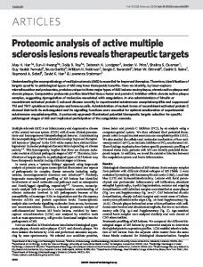
3. Description of Simulations [22] The model was run in one‐way nested mode from the globe to California/Nevada to Los Angeles (Figure 1). The domain horizontal resolutions were as follows: global (4°‐SN [stretched to 6° at the poles] × 5°‐WE), California/Nevada (Cal/Nev) (60 0.2° SN cells × 75 0.15° WE cells ≈ 21.5 km × 14.0 km with the SW corner cell centered at 30.0 oN and −126.0° W), and Los Angeles (46 0.045° SN cells × 70 0.05° WE cells ≈ 4.7 km × 5 km with the SW corner cell centered at 30.88 oN and −119.35° W). The global domain included 47 sigma‐pressure layers up to 0.22 hPa (≈60 km), with high resolution (15 layers) in the bottom 1 km. The nested regional domains included 35 layers exactly matching the global layers up to 65 hPa (≈18 km). The global, California/Nevada, and Los Angeles domains included 148,896, 157,500, and 112,700 grid cells, respectively. All physical processes, including gas photochemistry, were solved in all nested domains, including the global domain. [23] Two global‐urban nested simulations were run and compared with data: one with the 13,626‐reaction MCM and the other with the 327‐reaction MCBIV. Simulations were run from August 1–3, 2006 (72 h). The model was initialized on all scales with 1‐degree global reanalysis data (1° × 1° reanalysis fields, 2007, Global Forecast System, http://nomads.ncdc.noaa.gov/data/gfs‐avn‐hi/), but run without data assimilation, nudging, or model spinup. The time

5 of 13

D14304

JACOBSON AND GINNEBAUGH: LARGE‐MECHANISM 3‐D PHOTOCHEMISTRY

Figure 1. Locations of the three model domains (global, California/Nevada, and Los Angeles basin) used in this study and measurement sites used for model comparison (open circles) with data in Figure 2. interval for passing meteorological and chemical variables from one domain to the next was one hour.

4. Results [24] Table 3 summarizes statistics comparing model results with data from each the MCM and MCBIV simulations for the Los Angeles (L.A.) domain. Table 4 does the same for the California/Nevada (Cal/Nev) domain. Statistics include normalized gross errors (NGE) and normalized biases (NB). An NGE is the absolute value difference between the modeled and observed value, divided by the observed value, summed up over all observed values above a cutoff (given in the table), then divided by the number of such observed values. The NB is the same, but without taking absolute values, so always has a magnitude ≤ that of the NGE. Whereas, the NGE gives an indication of model accuracy, the NB gives an indication of whether the model under‐ or over‐predicted the data. Figure 2 shows paired‐in‐time‐ and‐space (PITS ‐ at the exact time and location of the measurement) comparisons of model results with data from each the MCM and MCBIV simulations for the L.A. and Cal/Nev domains. [25] Table 3 indicates that the ozone NGE was < 30% in the L.A. domain for both chemical mechanisms (26.6% for the MCM and 28.3% for the MCBIV), indicating general good agreement for both considering the difficulty of simulating ozone in Los Angeles particularly when meteorology and chemistry are predicted and feed back to each other. This also represents an improvement in the 68‐h NGE of 32.6% from Jacobson et al. [1996], which also included both meteorological and chemical prediction, for the same basin but for a different period. The ozone NGE was ∼2 percentage points more accurate for the MCM than for the MCBIV. In the Cal/Nev domain, ozone predictability also improved for the MCM versus the MCBIV, but by a smaller magnitude (∼0.4 percentage points). Of the paired‐in‐time‐ and‐space plots for ozone (Figures 2a.i, 2b.i, 2c.i, 2d.i‐iii), several reflect the relatively small difference in NGEs. The MCM predictions (solid lines) were often closer to the data

D14304

than were the MCBIV predictions, but there were also cases where the reverse was true. The plots indicate a relatively good match of peaks and diurnal variations in two or all three days at most of the locations shown. [26] Table 3 indicates that CO and NOx predictability improved with the MCM versus the MCBIV in both the Los Angeles and Cal/Nev domains. Since the inorganic chemical reactions were the same in both cases, the original cause of the difference must have been the improved explicitness of the organic reactions. Figures 2b and 2c show graphical comparisons at selected sites. The time series plots for CO (Figures 2a.ii, 2b.iii, 2d.v) and NO2 (Figures 2b.ii, 2c.ii, 2d.iv) indicate relatively little difference between the MCM and MCBIV results by hour although small differences can be seen. [27] Ethane, propane, ethene, and propene oxidation were treated explicitly in both the MCM and MCBIV chemical mechanisms with respect to their loss reactions. The MCM included chemical production sources of all four, whereas the MCBIV included chemical production sources of only ethane. The prediction accuracies of ethane (Tables 3 and 4 and Figures 2a.iii, 2d.vi) and propane (Tables 3 and 4 and Figures 2a.iv) were better for MCBIV in Los Angeles but better for MCM in California. Since the reaction loss of these two chemicals dominated their production, the loss reactions were similar in both cases, and both have relatively long lifetimes, it is not a surprise that the accuracies for these two chemicals were somewhat similar. The accuracies of ethene and propene were slightly better for MCM in both domains. A comparison of Figure 2a.v with Figure 2a.iii indicates that modeled differences between the MCM and MCBIV were larger for ethene than for ethane at the same location. A comparison of Figure 2a.vi with Figure 2a.iv indicates a similar result for propene versus propane. These results are expected since the lifetimes of ethane and propane are much longer than are those of ethene and propene, respectively. [28] Formaldehyde in the MCBIV is treated simultaneously as an explicit species and lumped bond group. In MCM, formaldehyde is produced and lost explicitly. Prediction accuracy of formaldehyde was better in the MCM than MCBIV in both domains although errors in the Cal/Nev domain became significant at a few locations where emissions were probably not characterized well. Figures 2b.iv, 2c.v, and 2d.vii show a good match between modeled and measured formaldehyde for both mechanisms at three locations in the Los Angeles domain. [29] Acetaldehyde in the original CBIV mechanism was also treated simultaneously as an explicit species and lumped bond group. However, for the MCBIV here, acetaldehyde was separated from other higher aldehydes and treated explicitly (but with much less complex photochemistry than in the MCM) and higher aldehydes were treated as their own lumped bond group. The reactions involving acetaldehyde and higher aldehydes in MCBIV are given by Jacobson [2008, supplement]. Acetone was also treated as an explicit species in the MCBIV. Acetaldehyde prediction accuracy was better for the MCM on the Cal/Nev domain but less accurate than the MCBIV on the L.A. domain (Tables 3 and 4 and Figures 2b.v, 2b.vi), and acetone accuracy was better for the MCBIV on both domains (Tables 3 and 4). Benzene (Figures 2d.xiii, 2d.ix), toluene (Figures 2d.x, 2d.xi), and

6 of 13

D14304

JACOBSON AND GINNEBAUGH: LARGE‐MECHANISM 3‐D PHOTOCHEMISTRY

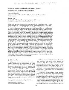
Figure 2. (a, b, c) Paired‐in‐time‐and‐space comparisons of modeled MCM (solid lines), modeled MCBIV (dashed lines), and data (dots) (AirData, 2006, U.S. Environmental Protection Agency, http:// www.epa.gov/air/data) for multiple gases each at three individual stations for the Los Angeles (L.A.) domain for August 1–3, 2006. For some chemicals, results are also shown for the California/Nevada domain (Cal/Nev) of the same simulation. Measurement sites are shown in Figure 1. For all plots except those showing OH, modeled values are shown at 1‐h intervals. For OH plots, values are shown at 4‐h intervals, explaining the sharpness of the gradients. (d) Same as Figures 2a−2c but for several gases at different stations for the Los Angeles (L.A.) domain for August 1–3, 2006. 7 of 13

D14304

D14304

JACOBSON AND GINNEBAUGH: LARGE‐MECHANISM 3‐D PHOTOCHEMISTRY

Figure 2. (continued) 8 of 13

D14304

D14304

D14304

JACOBSON AND GINNEBAUGH: LARGE‐MECHANISM 3‐D PHOTOCHEMISTRY

Table 3. Normalized Gross Errors (NGE) and Normalized Biases (NB) for Several Near‐Surface Chemicals From the Los Angeles Domain From Both the MCM and MCBIV Simulationsa MCM

MCBIV

Parameter

Cutoffb

Number of Observationsc

Number of Stationsc

NGE (%)

NB (%)

NGE (%)

NB (%)

Ozone Carbon monoxide Nitrogen dioxide Ethane Propane Ethene Propene Formaldehyde Acetaldehyde Acetone Benzene Toluene Isoprene PM2.5 PM10

50 100 20 1 1 3 1 3 1 1 1 1 3 0 0

402 993 261 43 39 12 11 43 60 63 20 37 2 36 146

43 25 28 7 8 6 7 5 5 5 7 8 7 19 5

26.6 53.3 68.8 57.1 90.1 35.1 57.2 47.3 58.1 79.7 81.3 76.1 65.5 43.7 54.8

14.4 27.3 49.2 −48.8 −90.1 −30.4 −57.2 35.9 −53.5 −79.7 −81.3 −73.7 −65.5 27.6 0.43

28.3 56.3 74.0 53.1 89.7 35.2 72.4 53.1 50.4 65.3 80.8 76.3 45.0 76.1 63.4

20.6 32.5 57.2 −48.6 −89.7 −7.5 −72.4 46.3 −18.7 −65.3 −80.8 −66.1 −45.0 69.2 34.3

a

NGE, normalized gross errors; NB, normalized biases. Units of ppbv for gases and mg/m3 for particulate matter. c The number of observations is the number above the cutoff. The number of stations is the number of stations with values above or below the cutoff. b

isoprene (Figures 2a.xiii, 2d.xii) prediction accuracy (Tables 3 and 4) were mixed between the two domains for the two mechanisms. It should be noted, however, that the number of data values available for these and several other organics was small (Tables 3 and 4). No data were available for OH, but daytime modeled values were only slightly higher for the MCBIV than for the MCM mechanisms (Figures 2a.iv, 2b.vii, 2c.vii ‐ provided only in 4‐h intervals). [30] PM2.5 and PM210 accuracy for the few data points available was fairly good for Los Angeles for the MCM, particularly considering no low cutoff was used to compare the model with data. However, while explicit inorganic gases grew onto size‐resolved aerosols accounting for competition between the gas and particle phases and accounting for different growth rates for particles of different size, explicit gases in the MCM were only lumped into a few groups for growth onto aerosol particles, and the groups were grown in a size‐resolved manner as with the inorganics. Since

the treatment of secondary organic gas‐to‐particle conversion is still a work in progress, we do not take much stock in the accuracy of the particulate matter results for Los Angeles. Particle prediction accuracy for California was not so good as in Los Angeles, primarily because many sites had low concentrations, and no low threshold was used in the error analysis, so differences at the low‐concentration sites dominated. [31] The 3‐D simulations performed here were evaluated against data and the MCBIV in Los Angeles, where NOx levels are fairly high in general. However, during the night and in remote areas of the basin, NOx levels decrease significantly. The results here (Table 3 and Figure 2) suggest that the MCBIV and MCM were relatively consistent with each other for most all conditions (day and night and in remote and urban areas). The relative agreement between the MCM and MCBIV is also consistent with the trajectory study of Derwent et al. [2005], who found that the MCM compared

Table 4. Normalized Gross Errors and Normalized Biases for Several Near‐Surface Chemicals From the California/Nevada Domain From Both the MCM and MCBIV Simulationsa MCM

MCBIV

Parameter

Cutoffb

Number of Observationsc

Number of Stationsc

NGE (%)

NB (%)

NGE (%)

NB (%)

Ozone Carbon monoxide Nitrogen dioxide Ethane Propane Ethene Propene Formaldehyde Acetaldehyde Acetone Benzene Toluene Isoprene PM2.5 PM10

50 100 20 1 1 3 1 3 1 1 1 1 3 0 0

2911 4091 545 45 57 12 16 48 65 71 25 54 5 70 1407

185 77 98 9 12 8 11 7 8 7 10 12 10 51 53

30.3 68.1 96.4 69.6 82.0 38.3 76.8 170.8 56.8 58.0 79.2 93.0 44.4 80.9 91.9

4.7 30.5 52.9 5.2 −78.8 −30.3 −39.3 167.7 −0.8 −56.2 −79.2 −43.3 −17.6 76.4 55.6

30.7 68.5 103.5 77.0 82.3 38.4 82.5 192.4 105.3 40.8 78.3 108.6 47.1 110.3 111.8

8.4 30.9 59.6 16.4 −77.9 6.7 −60.8 189.1 84.9 −30.4 −78.3 −22.7 −17.3 109.2 85.0

a

NGE, normalized gross errors; NB, normalized biases. Units of ppbv for gases and mg/m3 for particulate matter. c The number of observations is the number above the cutoff. The number of stations is the number of stations with values above or below the cutoff. b

9 of 13

D14304

JACOBSON AND GINNEBAUGH: LARGE‐MECHANISM 3‐D PHOTOCHEMISTRY

well with another lumped carbon bond mechanism under Northern‐European NOx conditions.

5. Computer Timings [32] Ginnebaugh et al. [2010] discuss the 3‐D computer time of three MCM versions of different size and of a version of the MCBIV similar to that used here when all were run using SMVGEAR II with photochemistry alone. Figure S2 of that paper, for example, indicates that a 4649‐species version of the MCM required only 8.1 times more computer time than a 140‐species MCBIV (1/33rd the size) when both were run in 500 grid cells. The relative speed improvement of any large versus small mechanism in SMVGEAR II is due to the sparse‐matrix and array‐referencing techniques in the code [Jacobson, 1998]. Ginnebaugh et al. [2010] quantify the number of multiplication reductions due to sparse‐matrix techniques between the MCM and MCBIV. [33] For the present study, 3‐D simulations accounting for gas, aerosol, cloud, dynamical, radiative, ocean, and land surface processes were run on only four Intel Xeon dual‐core 5260 3.33 GHz processors and using only one core and 22 GB of memory per processor, with Infiniband interconnections. The overall computer time required for simulations on three nested domains was 1.75 days per day of simulation for the MCBIV mechanism and 6.45 days per day of simulation for the MCM mechanism. Thus, despite the factors of 31 and 46 increases in the numbers of species and reactions, respectively, due to the MCM versus MCBIV, the overall computer time (accounting for all model processes) required for GATOR‐GCMOM with MCM was only ∼3.7 times that with the MCBIV. [34] With the MCBIV, photochemistry required ∼15% of the overall computer time in GATOR‐GCMOM. As discussed above, the time required for photochemistry alone with MCM is ∼8.1 times that with MCBIV. Thus, MCM photochemistry alone accounted for only a doubling of overall GATOR‐ GCMOM computer time relative to MCBIV. However, MCM species affected computer time not only by taking part in photochemistry (in SMVGEAR II) but also by taking part in spectrally integrated heating rate and photolysis calculations, advection, convection in air, convection in cumulus clouds, diffusion, gas‐cloud and gas‐precipitation dissolution, wet deposition, dry deposition, and ocean‐atmosphere exchange. These other processes accounted for the remainder of the computer time increases. Most of this additional time was due to advection/convection/diffusion in air and clouds, which was calculated every 5 min. In sum, the overall computer time with MCM in a coupled model was only 3.7 times that of MCBIV, small relative to the factor of 33 increase in the number of species treated. This suggests that computer speed is no longer a barrier to the 3‐D simulation of photochemistry with the MCM or similar mechanisms when a fast and stable solver of chemical equations is used.

6. Implications [35] Although the computational barrier against solving atmospheric photochemistry with on the order of 13,000 reactions in a 3‐D model has been overcome, further work is needed to complete and test large mechanisms and in developing accurate emission inventories for them.

D14304

[36] The results here further suggest that the accuracy of the condensed photochemical mechanism used (MCBIV), with 31 times fewer species and 46 times fewer reactions than MCM, was not the limiting factor in the simulation of ozone air pollution. More likely factors limiting ozone prediction accuracy are emissions and meteorological variable prediction (e.g., boundary layer heights, temperatures, wind speeds and direction), although this is not proven here. Whereas, the MCM improved ozone prediction accuracy only a small amount in 3‐D, it should improve the ability of modelers to focus efforts on developing more explicit treatments of secondary organic matter (SOM) formation, an important goal [e.g., Utembe et al., 2009]. Such developments are foreseen, since current methods of solving for SOM in 3‐D all involve lumping of organics and solving growth based on lumped‐species vapor pressures and solubilities. More‐explicit treatment of gases and gas chemistry will allow for more‐explicit model treatment of growth and dissolution based on species‐specific vapor pressure and solubility data and of more explicit treatment of aqueous chemistry. A difficulty with treating more‐explicit SOM formation will be in evaluating the results. To this end, additional chamber experiments tracing the pathway of emitted gases to their secondary aerosol production would be beneficial. Field experiments with more explicit differentiation of SOM products would also be helpful. [37] A more‐explicit mechanism also allows for a more complete calculation of ultraviolet (UV) radiation reduction and atmospheric heating rates by gases and aerosol particles. All photolyzing gases attenuate UV (and some attenuate visible) radiation, thereby enhancing heating rates. Jacobson [1999] calculated that a selected set of nitrated aromatic gases reduced UV radiation by 2‐3% in Claremont and Riverside, California (reducing total solar by ∼0.1%) during a 1987 episode, feeding back to ozone production. Nitrated and aromatic aerosols were found to have caused larger UV reductions, explaining much of the 33–48% observed UV reductions in Claremont and Riverside. The explicit treatment of absorbing organic gases, particularly nitrated aromatics, aldehydes, benzoic acids, aromatic polycarboxylic acids, phenols, and polycyclic aromatic hydrocarbon, and their conversion to aerosol, should help to improve the calculation of gas and aerosol UV attenuation and its feedback to air pollution. [38] Figure 3 illustrates some of the feedback differences resulting from the use of the MCBIV versus the MCM mechanisms. The two mechanisms affected meteorology differentially for two reasons. First, the model (Section 2.3) treated spectral absorption by all radiatively active gases, and such absorption affected photolysis coefficients and heating rates at all altitudes. The MCM included many more explicit species for which absorption could be calculated than did the MCBIV, since absorption in the MCBIV was calculated only for explicit species, not for lumped bond groups. Second, the model treated gas‐to‐particle conversion of many gases (e.g., HNO3, H2SO4, HCl, NH3, some organics), so differences in modeled gas concentrations due to photochemistry between the mechanisms could affect aerosol concentrations, thus clouds and other meteorological variables. [39] Figure 3a indicates that heating rates due to absorption in the lower troposphere were 1–6% higher in the MCM than in the MCBIV case, as expected due to the larger

10 of 13

D14304

JACOBSON AND GINNEBAUGH: LARGE‐MECHANISM 3‐D PHOTOCHEMISTRY

D14304

Figure 3. (a−h) Simulation‐ and domain‐averaged vertical‐profile differences and percent differences between the MCM and MCBIV simulations for several variables. (i) Same as Figures 3a−3h but for the simulation‐averaged surface difference in downward UV ( 110 explicit organic gases and all important inorganic gases from tens of thousands of mobile, point, and area sources were derived from the 2005 U.S. EPA National Emission Inventory. [42] Model results were compared with paired‐in‐time‐ and‐space data in both the Los Angeles and California domains for a 3‐day air pollution episode and with results obtained from a modified Carbon‐Bond IV mechanism (MCBIV) of 152 species and 297 reactions. Results indicate that the more‐explicit mechanism reduced the normalized gross error (NGE) of ozone against data for the simulation period over the CBIV‐Ex by only ∼2 percentage points (from 28.3% to 26.5%) and nitrogen dioxide and formaldehyde by ∼6 percentage points in Los Angeles. While more‐explicit photochemistry improved overall chemical results slightly, use of the condensed mechanism was not the main source of model error. However, the more‐explicit treatment of gases may improve the ability of modelers to focus efforts on developing more explicit treatments of secondary organic matter formation. More explicit treatment should also improve the simulation of gas plus aerosol UV radiation reduction. Radiation absorption by short‐ lived gases feeds back to meteorology and climate, feeding back in turn to the gases themselves. The more explicit mechanism, which treated absorptive heating by more photolyzing gases, resulted in a different magnitude of feedbacks to meteorological variables and back to gases themselves, than did the less‐explicit mechanism. As such, further modeling efforts using more explicit photochemistry should continue. The overall computer time (accounting for all model processes) required for the nested GATOR‐ GCMOM model to solve the more‐explicit photochemistry with SMVGEAR II was only ∼3.7 times that required to solve the MCBIV mechanism despite the factors of 31 difference in number of species and 46 difference in number of reactions. [43] Acknowledgments. Support came from the U.S. Environmental Protection Agency grant RD‐83337101‐O, NASA grant NX07AN25G, the NASA High‐End Computing Program, and the Department of the Army Center at Stanford University.

D14304

References Andreae, M. O., and P. Merlet (2001), Emission of trace gases and aerosols from biomass burning, Global Biogeochem. Cycles, 15, 955–966, doi:10.1029/2000GB001382. Aumont, B., S. Szopa, and S. Madronich (2005), Modelling the evolution of organic carbon during its gas‐phase tropospheric oxidation: Development of an explicit model based on a self generating approach, Atmos. Chem. Phys., 5, 2497–2517, doi:10.5194/acp-5-2497-2005. Austin, J., and N. Butchart (1992), A three‐dimensional modeling study of the influence of planetary wave dynamics on polar ozone photochemistry, J. Geophys. Res., 97, 10,165–10,186. Bates, D. R., and M. Nicolet (1950), The photochemistry of atmospheric water vapor, J. Geophys. Res., 55, 301–327, doi:10.1029/JZ055i003p00301. Chapman, S. (1930), On ozone and atomic oxygen in the upper atmosphere, Philos. Mag., 10, 369–383. Crutzen, P. J. (1971), Ozone production rates in an oxygen‐hydrogen‐nitrogen oxide atmosphere, J. Geophys. Res., 76, 7311–7327, doi:10.1029/ JC076i030p07311. Derwent, R. G., M. E. Jenkin, S. M. Saunders, M. J. Pilling, and N. R. Passant (2005), Multi‐day ozone formation for alkenes and carbonyls investigated with a master chemical mechanism under European conditions, Atmos. Environ., 39, 627–635, doi:10.1016/j.atmosenv.2004.10.017. Gear, C. W. (1969), The automatic integration of stiff ordinary differential equations, in Information Processing, 68, edited by A. J. H. Morrel, pp. 187–193, North‐Holland, Amsterdam. Gery, M., G. Z. Whitten, J. Killus, and M. Dodge (1989), A photochemical kinetics mechanism for urban and regional computer modeling, J. Geophys. Res., 94, 12,925–12,956, doi:10.1029/JD094iD10p12925. Ginnebaugh, D. L., J. Liang, and M. Z. Jacobson (2010), Examining the temperature‐dependence of ethanol (E85) versus gasoline emissions on air pollution with a largely explicit chemical mechanism, Atmos. Environ., 44, 1192–1199, doi:10.1016/j.atmosenv.2009.12.024. Gong, W., and H.‐R. Cho (1993), A numerical scheme for the integration of the gas‐phase chemical rate equations in three‐dimensional atmospheric models, Atmos. Environ. Part A, 27A, 2147–2160. Griffin, R. J., D. Dabdub, and J. H. Seinfeld (2002), Secondary organic aerosol: 1. Atmospheric chemical mechanism for production of molecular constituents, J. Geophys. Res., 107(D17), 4332, doi:10.1029/ 2001JD000541. Hesstvedt, E., O. Hov, and I. S. A. Isaksen (1978), Quasi‐steady‐state approximations in air pollution modeling: Comparison of two numerical schemes for oxidant prediction, Int. J. Chem. Kinet., 10, 971–994, doi:10.1002/kin.550100907. Hunt, B. G. (1966), Photochemistry of ozone in a moist atmosphere, J. Geophys. Res., 71, 1385–1398. Jacobson, M. Z. (1998), Vector and scalar improvement of SMVGEAR II through absolute error tolerance control, Atmos. Environ., 32, 791–796, doi:10.1016/S1352-2310(97)00315-4. Jacobson, M. Z. (1999), Isolating nitrated and aromatic aerosols and nitrated aromatic gases as sources of ultraviolet light absorption, J. Geophys. Res., 104, 3527–3542, doi:10.1029/1998JD100054. Jacobson, M. Z. (2001), GATOR‐GCMM: A global through urban scale air pollution and weather forecast model: 1. Model design and treatment of subgrid soil, vegetation, roads, rooftops, water, sea ice, and snow, J. Geophys. Res., 106, 5385–5402, doi:10.1029/2000JD900560. Jacobson, M. Z. (2005), A refined method of parameterizing absorption coefficients among multiple gases simultaneously from line‐by‐line data, J. Atmos. Sci., 62, 506–517, doi:10.1175/JAS-3372.1. Jacobson, M. Z. (2008), Effects of wind‐powered hydrogen fuel cell vehicles on stratospheric ozone and global climate, Geophys. Res. Lett., 35, L19803, doi:10.1029/2008GL035102. Jacobson, M. Z., and D. G. Streets (2009), The influence of future anthropogenic emissions on climate, natural emissions, and air quality, J. Geophys. Res., 114, D08118, doi:10.1029/2008JD011476. Jacobson, M. Z., and R. P. Turco (1994), SMVGEAR: A sparse‐matrix, vectorized gear code for atmospheric models, Atmos. Environ., 28, 273–284, doi:10.1016/1352-2310(94)90102-3. Jacobson, M. Z., R. Lu, R. P. Turco, and O. B. Toon (1996), Development and application of a new air pollution modeling system. Part I: Gas‐phase simulations, Atmos. Environ., 30, 1939–1963, doi:10.1016/1352-2310 (95)00139-5. Jacobson, M. Z., Y. J. Kaufmann, and Y. Rudich (2007), Examining feedbacks of aerosols to urban climate with a model that treats 3‐D clouds with aerosol inclusions, J. Geophys. Res., 112, D24205, doi:10.1029/ 2007JD008922. Jenkin, M. E., S. M. Saunders, and M. J. Pilling (1997), The tropospheric degradation of volatile organic compounds: A protocol for mechanism development, Atmos. Environ., 31, 81–104, doi:10.1016/S1352-2310 (96)00105-7.

12 of 13

D14304

JACOBSON AND GINNEBAUGH: LARGE‐MECHANISM 3‐D PHOTOCHEMISTRY

Jenkin, M. E., L. A. Watson, S. R. Utembe, and D. E. Shallcross (2008), A Common Representative Intermediates (CRI) mechanism for VOC degradation. Part 1: Gas phase mechanism development, Atmos. Environ., 42, 7185–7195, doi:10.1016/j.atmosenv.2008.07.028. Liang, J., and M. Z. Jacobson (2000), Comparison of a 4000‐reaction chemical mechanism with the carbon bond IV and an adjusted carbon bond IV‐EX mechanism using SMVGEAR II, Atmos. Environ., 34, 3015–3026, doi:10.1016/S1352-2310(99)00486-0. Madronich, S., and J. G. Calvert (1990), Permutation reactions of organic peroxy radicals in the troposphere, J. Geophys. Res., 95, 5697–5715, doi:10.1029/JD095iD05p05697. McRae, G. J., W. R. Goodin, and J. H. Seinfeld (1982), Development of a second‐generation mathematical model for urban air pollution—I. Model formulation, Atmos. Environ., 16, 679–696, doi:10.1016/0004-6981(82) 90386-9. Odman, M. T., N. Kumar, and A. G. Russell (1992), A comparison of fast chemical kinetic solvers for air quality models, Atmos. Environ. Part A, 36, 1783–1789. Reynolds, S. D., P. M. Roth, and J. H. Seinfeld (1973), Mathematical modeling of photochemical air pollution—I: Formulation of the model, Atmos. Environ., 7, 1033–1061, doi:10.1016/0004-6981(73)90214-X. Roth, P. M., S. D. Reynolds, P. J. W. Roberts, and J. H. Seinfeld (1971) Development of a simulation model for estimating ground‐level concentrations of photochemical pollutants, Rep. SAI 71/21, Syst. Appl., Inc., San Rafael, Calif. Russell, A. G., K. F. McCue, and G. R. Cass (1988), Mathematical modeling of the formation of nitrogen‐containing air pollutants. 1. Evaluation of an Eulerian photochemical model, Environ. Sci. Technol., 22, 263– 271, doi:10.1021/es00168a004. Sander, S. P., et al. (2006), Chemical kinetics and photochemical data for use in atmospheric studies: Evaluation number 15, JPL Publ., 06‐2, 523 pp. Sandu, A., J. G. Verwer, J. G. Blom, E. J. Spee, G. R. Carmichael, and F. A. Potra (1997), Benchmarking stiff ODE solvers for atmospheric chemistry problems II: Rosenbrock solvers, Atmos. Environ., 31, 3459–3472, doi:10.1016/S1352-2310(97)83212-8.

D14304

Saunders, S. M., M. E. Jenkin, R. G. Derwent, and M. J. Pilling (2003), Protocol for the development of the Master Chemical Mechanism, MCM v3(Part A): Tropospheric degradation of non‐aromatic volatile organic compounds, Atmos. Chem. Phys., 3, 161–180, doi:10.5194/ acp-3-161-2003. Shimazaki, T., and A. R. Laird (1970), A model calculation of the diurnal variation in minor neutral constituents in the mesosphere and lower thermosphere including transport effects, J. Geophys. Res., 75, 3221‐3235, doi:10.1029/JA075i016p03221. Szopa, S., B. Aumont, and S. Madronich (2005), Assessment of the reduction methods used to develop chemical schemes: Building of a new chemical scheme for VOC oxidation suited to three‐dimensional multiscale HOx‐NOx‐VOC chemistry simulations, Atmos. Chem. Phys., 5, 2519–2538, doi:10.5194/acp-5-2519-2005. Toon, O. B., C. P. McKay, T. P. Ackerman, and K. Santhanam (1989), Rapid calculation of radiative heating rates and photodissociation rates in inhomogeneous multiple scattering atmospheres, J. Geophys. Res., 94, 16,287–16,301, doi:10.1029/JD094iD13p16287. Turco, R. P., and R. C. Whitten (1974), A comparison of several computational techniques for solving some common aeronomic problems, J. Geophys. Res., 79, 3179–3185, doi:10.1029/JA079i022p03179. Utembe, S. R., L. A. Watson, D. E. Shallcross, and M. E. Jenkin (2009), A Common Representative Intermediates (CRI) mechanism for VOC degradation. Part 3: Development of a secondary organic aerosol module, Atmos. Environ., 43, 1982–1990, doi:10.1016/j.atmosenv.2009.01.008. Wulf, O. R., and L. S. Deming (1936), The theoretical calculation of the distribution of photochemically formed ozone in the atmosphere, Terr. Magn. Atmos. Electr., 41, 299–310, doi:10.1029/TE041i003p00299. D. L. Ginnebaugh and M. Z. Jacobson, Department of Civil and Environmental Engineering, Stanford University, Stanford, CA 94305‐4020, USA. ([email protected])

13 of 13