MOTOYASU NAGATA, MEMBER, IEEE, KENJI TAKADA, AND MAMORU SAKUDA. Abstract-A new correction method is investigated for distorted measurement ...
IEEE TRANSACTIONS ON BIOMEDICAL ENGINEERING, VOL. BME-33, NO. 12, DECEMBER 1986
1213
Correction Modeling of Distorted Signals Recorded by Mandibular Kinesiograph
GMDH
MOTOYASU NAGATA,
MEMBER, IEEE,
KENJI TAKADA,
Abstract-A new correction method is investigated for distorted measurement signals recorded by a mandibular kinesiograph, an electromagnetic device to quantify jaw movement by a magnetic transducer fixed on the mandible. The method employs a self-organized system identification known as a group method of data handling (GMDH). The proposed GMDH correction method has the capability to design a two-dimensional nonlinear autoregressive model which represents the relationship between distorted measurements and their corrected estimates of the mandibular displacement for the initial adjustment of kinesiographic signals under ferromagnetic influences. A computational procedure of a GMDH correction method is described in which the mathematical structure of a nonlinear autoregressive model is identified in a self-organized manner. Heuristic determination of a restricted sensor array zone of a kinesiograph is proposed to obtain effective fitness of a particular GMDH correction model which corresponds to each of the concomitant restricted zones. Corrected signals evaluated in the present study reveal a mean estimation error of 0.101 mm with a standard deviation of 0.125 mm which is regarded as highly accurate in a clinical sense.
INTRODUCTION UANTITATIVE assessment of mandibular displacement patterns during oral functions has been considere indispensable in current dentistry for the establish-
ment of precise diagnostic and treatment regimen for patients with malocclusions and mandibular dysfunctions. A mandibular kinesiograph has been used to quantify functional movement of the mandible in space [3]. The performance of a kinesiograph is characterized by its minimum loading on the mandible which facilitates analysis of mandibular movement under physiologic conditions together with its relative noninvasiveness to oral tissues and physical ease of operation [7]. However, since the principle of a kinesiograph is to determine change in magnetic environment when a magnetic transducer fixed on the inferior part of mandibular incisors is displaced in accordance with mandibular movement, the distortion of signals recorded by this device, essentially due to ferromagnetic interferences in measurement environment, has been claimed and several geometric correction models have been proposed [5], [7], [9]. Since these types of modeling are "deterministic" in a sense that they assume Manuscript revised September 29, 1986. This work was supported by Grant-in-Aid 60570956 from the Ministry of Education, the Government of Japan. M. Nagata is with the Faculty of Engineering, Osaka Electro-Communication University, Neyagawa, Osaka, Japan 572. K. Takada and M. Sakuda are with the Faculty of Dentistry, Osaka University, Suita Osaka, Japan 565. IEEE Log Number 8611639.
AND
MAMORU SAKUDA
mathematical structures of a model a priori, the self-adjustment capability according to the difference in measurement environment has been limited. In contrast, the group method of data handling (GMDH) which enables adaptive construction of a mathematical model has been proposed as a general system identification methodology [1], [2], and a previous report [10] from our laboratory has confirmed possible application of this method to the correction of kinesiographic data obtained in clinical environment. The purpose of the present paper is to provide a new correction method for distorted measurement signals recorded by a mandibular kinesiograph based on the GMDH, which has the capability to build a mathematical structure of a nonlinear autoregressive model which represents the relationship between distorted measurements and their corrected estimates in a self-organized manner. The performance of the GMDH correction method is also evaluated in an experimental environment. Three points are emphasized: first, a computational procedure of a GMDH correction method is described where system structure and coefficients of a nonlinear autoregressive model are identified simultaneously without knowledge of model structure. Second, heuristic determination of a restricted sensor array zone of a kinesiograph is proposed to obtain effective fitness of a particular GMDH correction model which corresponds to each of the concomitant restricted zones. Third, effectiveness of the currently proposed correction method is discussed in terms of computational procedure and experimental results with respect to correction accuracy and relevant properties. EXPERIMENTAL SYSTEM
Mandibular kinesiograph (K5-R, Myotronics Research Inc., WA) consists of a light head-frame which supports a set of magnetometers and is fixed on the patient's head by means of a spectacle-like device [10]. When it is applied in a clinical environment, magnetometers are aligned so that they could sense the linear movement of a magnet transducer in space with reference to a plane parallel to Frankfort horizontal plane, a coronal plane perpendicular to the Frankfort horizontal plane, and the midsagittal plane. A magnet transducer is attached to the labial surface of lower central incisors and the aforementioned three reference planes are arranged to meet in the center of the magnet when it is in its zeroed, i.e., habitual intercuspal position.
0018-9294/86/1200-1213$01.00 © 1986 IEEE
1214
IEEE TRANSACTIONS ON BIOMEDICAL ENGINEERING, VOL. BME-33, NO. 12, DECEMBER 1986
A brass-made sliding device fixed on the table of a three-dimensional digitizer (Gradicon) is connected to a cursor which, in turn, is linked to an aluminum bar. Since the alignment of the sensor array can affect the accuracy of measurement signals significantly, the magnet transducer is carefully positioned relative to the sensor array. A magnet is placed in a slot on the edge of the bar so that it could be displaced parallel to each of three axes determined by the sensor array of the kinesiograph. The long axis of the magnet transducer is arranged in parallel with a line which connected two lateral sensors. A detailed description of the current experimental system has been completed [10]. Measurement is made at lattice points with a 5 mm interval within a framework of -15 to 15 mm in the x direction (lateral), -10 to 20 mm in the y direction (anteroposterior) and 0 to -40 mm in the z direction (vertical). The origin is defined as a midpoint between two lateral sensors which corresponds to the intercuspal position of the mandibular incisor point in a clinical environment. Nominal x, y, and z coordinates of each lattice point are determined by the Gradicon to 0.01 mm together with a simultaneous recording of dc voltages by means of a digital tester for three directions obtained through the output connectors of the kinesiograph. The dc voltages are then converted to millimeters with a calibration of 200 mV = 1.00 mm and provide distorted X, Y, and Z coordinates for concomitant nominal values. For simplicity of description, three-dimensional coordinates are expressed by integers with decimal points and places abbreviated, e.g., (0, 5, 10) for (0.00 mm, 5.00 mm, 10.00 mm), in the present study. A total of 87 points in the aforementioned measurement area are selected for estimation. These points correspond to the following nominal coordinates, each of which ranges in six Cartesian products X x Y x Z with 1) X= (0, -5, -10), Y= -5,Z= (-5, -10, -15, -20), 2) X = (0, -5), Y = (0, 5), Z = (-5, -10, -15, -20, -25, -30, -35), 3) X = (0, -5), Y = 15,Z= (-15, -20, -25, -30,
model building process. The GMDH can build an autoregressive polynomial fitting model between input data and output data whose relationship is expressed as a multilayered network structure, where each layer generates the intermediate signal estimates of output variables of the overall object system. The intermediate estimate is an output of a nonlinear function of the present layer whose two input variables are selected from among output variables in the preceding layer. The nonlinear function is usually a second-order polynomial. Several elements are selected from among intermediate signal estimates by using self-selection threshold and allowed to proceed to the succeeding layer. Through a multilayered network structure, a mathematical model of a polynomial type which is the overall input-output transformation can be obtained with a model structure and its weighting coefficients. In other words, the concept of the GMDH modeling is a combination of regression analysis and decision regularization without any model assumptions based on engineering and/or dental considerations. In contrast to a single layered statistical or physical model, the GMDH model of multilayered network structure can design a complex system whose causality between input and output data is not elucidated to be ruled by a compact physical or biological law. The GMDH is thus introduced in the present correction strategy because of complex causality of the distortion of kinesiographic signals. The GMDH correction model of the mandibular kinesiograph represents the input-output relationship by the following polynomial functions. x ij =I (Xi-,j 1Xi-l,j, Xilj1
, X j+,j Xi+lj +1)
*
(1)
Yi,j
f2(Yim-1j, Y-ij
i
1
Zi,j = 3(ZT-l,J -1IZiT1 1J Z_
j+ 1
m
+ 1jYi+
I
j+) (2)
Zi+1Jj,zi+l j+l) (3)
where 4,, 91,J, and 2Cj are positional corrected estimates whose nominal coordinates are XC, yCj, and z4, respec-35) 4) X = (0, -5, -10), Y = 10,Z= (-10, -15, -20, tively. The variables xl j, y7,, and zT, are kinesiographic measurements which represent the position of a magnet -25, -30, -35), 5) X = -10, Y= (0, 5), Z = (-5, -10, -15, -20, transducer in space (Fig. 1). The problem of the GMDH -25, -30, -35), and modeling is to determine the unknown mathematical = = = X Z -25, -10, Y 6) 15, (-15, -20, -30, structure fl( ), f2( ), and f3( ) from the available mea-35), respectively. surements. The computational procedure of a GMDH correction The points are selected based on the assumption that their distribution in space unilaterally approximates man- modeling is described in the following algorithm from dibular positions at rest and during clenching and chew- Step 1 to Step 6 (Fig. 2). ing. Step 1: Without loss of generality, we focus on the modeling of the nonlinear polynomial (1). When x J is the GMDH CORRECTION MODEL estimate of the position of a magnet transducer of a kiThe GMDH is a self-organized modeling method of the nesiograph, the sensor array zone for model building is polynomial autoregression model by a combination of in- selected from the x-y plane or the x-z plane. In the first put variables in which the model order and coefficient pa- layer of the GMDH model, the following nine variables rameters are not assumed a priori but identified during the are input.
NAGATA et al.: GMDH MODELING OF SIGNALS BY MANDIBULAR KINESIOGRAPH
1215
Fig. 1. Diagrammatic drawing which illustrates measurements (xT-, yT.), nominal coordinates (x4j, yr), and estimates (x ;, 9 j) of kinesiograph in X-Y plane.
-Ii
* * Um.*Eliul ,
-,*tj
)*
doe(
|
*
s )ri IjI1*Ul 402 406'S*012) xm
), i
*
*
I0 s ;t aye r ( Gerate kir
()Con)pare
0
0
0
0
0
0
*
C. initermiediate performatien
*
2
*
qW
*
e
initermediate
s
t
~y
~(
variables
criteria
Fig. 2. Multilayered structure of GMDH algorithm.
u(1)
= Xi
u(4)
=
xi,-1,
u(7)
=
x'+
,
Tl,
u(2)
=
x
u(5)
=
xi
.,
u(8) = x7+,j
u(3)
=
Xi
u(6)
=
Xi
U(9)
=
X+ (4)
a =
(a,,
+
uk(2)
=
alu(I)
+ a2U(3) +
a2U(2)
+
a3U(M) u(2) a3U(M) u(2) (5)
where these intermediate variables u k(i) (i = 1, 2, 9C2) are candidates for the estimate x, in the kth layer. It should be noticed that coefficient parameters an(n = 1, 2, 3) are identified for 9C2 cases which correspond to u k(i)
5 th L Iday
" ) eles ict-
alu(I)
uk( C2) = alu(8) + a2u(9) + a3u(8) u(9),
~
variabk.
=
GO)2)
1184
0
(IV Lay
2n
-
Ul .U
*
0
92 0
m
*
0
~~~~11~ Xi,.,,* -*L9'u80 x
0
Lf3)-*
I'ji
uk(l)
(i = 1, 2, 9, C2) and these parameters are calculated in Step 3. Step 3: For all combinations of input variables u(i) and u(j), calculate identified coefficients an(n = 1, 2, 3) in order to minimize the mean-square error. J(i,j) = (1/N)E(xc -alu(i) -a2u(j) - a3u(i) U(j))2. (6) Coefficient parameters are obtained from the Gauss normal equation Ma = b, (7) where
a2, a3)T
(8)
F(1IN)2u2(i), (1IN)2u(i) u(j), (1IN)9u2(i) u(j)
M
=
b
=
(l/N)Eu(i) u(j), (l/N)Yu2(j), (l/N)2u(i) u2(j) (l/N)Fu2(i) U j), (lNN)xu(i) u2(j),(N1N)Eu2(i) u2(j) ((lIlN)Exl, u(i), (l1lN)Exl,-u( j), (l1lN)ExC jU(i) uf j))T.
(9)
(10)
Calculate 9C2 intermediate variables u k(i) (i = 1, where xT, represents the distorted signal of a nominal co- 9C2) by using parameters an(n = 1, 2, 3) which correordinate of x4;. Set k = 1. spond to uk(i) Step 2: Generate 9C2 intermediate variables each of Step 4: Among 9C2u'(i)s, select nine intermediate varwhich is the output of the nonlinear polynomial iables u(i)s whose estimation error criteria are the inside
1216
IEEE TRANSACTIONS ON BIOMEDICAL ENGINEERING, VOL. BME-33, NO. 12, DECEMBER 1986
best nine. Sort selected variables in the ascendant order of criteria and renumber them in a numerical order from u(1) to u(9). Set k + 1 as k. Step 5: Check whether the minimum estimation error criterion is smaller than the estimation error criterion in the one-step preceding layer. If this condition is satisfied, then go to Step 2. If not, stop calculation. Step 6: The most identified GMDH correction model of mandibular kinesiograph can be obtained by backtracking from the best intermediate variable of the final layer. Thus, the best-fitted corrected estimate is expressed as a polynomial of the measurements and a mathematical structure fl( ) can be determined. ZONING Restricted sensor array regions of a kinesiograph are determined heuristically to obtain effective fitness of a particular GMDH model whose estimates correspond to nominal coordinates of the restricted zone. The particular GMDH model can be built based on measurements of the specified zone and its directly adjoining zone. Zoning is performed to condition a two-dimensional rectangle area on a plane which is perpendicular to one of x, y, or z axes. It should be noticed that different zones may be assigned according to the positional coordinate to be estimated even with the same plane fixed. For example, in a condition where the fixed plane is Y = 5, the zones may be different depending on whether the coordinate to be estimated is X or Z. Furthermore, two determined zones may be overlapped partly on the same plane even if positional coordinates to be estimated are identical. According to circumstances, two different GMDH models may be applied to partly overlapped zones. The more fitted estimate may be selected from the two estimates of the two GMDH models for the correction of coordinates in partly overlapped zones. The particular GMDH model of a restricted zone is characterized by the mathematical structure of polynomial and its weighting coefficients, which is a nonlinear autoregressive model in the correction of kinesiographic signals of a conditioned zone. Corrected estimates and estimation errors are obtained for the total of 261 coordinates (87 lattice points) in the correction zone. RESULTS
Table I gives distribution of estimation errors for all the x, y, and z coordinates estimated. 172 coordinates reveal estimation errors smaller than 0.1 mm. 54 coordinates reveal the errors of between 0.1 and 0.2 mm. Approximately 92 percent of the corrected coordinates (241 coordinates) reveal estimation errors smaller than 0.3 mm, while 0.8 percent of them (two coordinates) show errors of between 0.6 and 0.8 mm. The mean estimation error for all 261 coordinate values is 0.101 mm with a standard deviation of 0.125 mm. The maximum estimation error is 0.790 mm for the Y coordinate of a nominal point (-5, 5, -10), whereas the minimum is 4.29 x 10⁻⁶ mm for the Y coordinate of a nominal point (-10, 5, -10).
DISTRIBUTION
OF
TABLE I ESTIMATION ERRORS FOR 261 COORDINATES
INominal-Estimate (mm) 0.1 0.1- 0.2 0.2- 0.3 0.3- 0.4 '0.4 - 0. 5 0.5- 0.6 0.6- 0.7 0.7- 0.8
Coordinate z Y
x 52 15
4
9 4 2 0 1
87
58 18 8 2
a
0 0 1 87
Frequency
(Incidence%)
3 0 0 1
0 0
172(65.9) 54(20.7) 15( 5.8) 11( 4.2) 4( 1.5) 3( 1.2) 0( 0.0) 2( 0.8)
87
261(100)
62 21
Y= 0
x
Fig. 3. Diagrammatic illustration of zoning to determine X coordinate estimates on the X-Z plane at the level of Y = 0.
As for X coordinates, 82 percent of 87 coordinates reveal the errors smaller than 0.3 mm with the maximum error of 0.747 mm for the point (0, 0, -10). With regard to Y coordinates, 97 percent of them take the estimation errors smaller than 0.3 mm. The maximum error for Y coordinates is 0.790 mm for the point (-5, 5, -10). In addition the errors smaller than 0.3 mm are identified in 99 percent of Z coordinates. The maximum error for Z coordinates is 0.506 mm for the point (-10, 10, -15). The selected zone is regarded as the area in which correction is performed by a specified GMDH model (Figs. 3-11). In other words, the correction model is consistent for all lattice points of, the specified zone in a mathematical sense. In case of X coordinate estimates with the Y axis fixed, it is observed that most zoning areas consist of two lattice points with a few exceptions which include three lattice points. It is also observed that 11 zones {(-5) X (-5), (-5) x (-10), (-5) x (-15), (-5) x (-20)} C X x Z overlap for Y = 0 and Y = 5 and partly overlap for Y = 10. Four zones {(-5) x (-5, -10), (-5) x (-15, -20)} C X x Z overlap for Y = 0 and Y = 5, and two zones {(-5) x (-10, -15), (-5) x (-20, -25)} C X x Z for Y = 10 overlap obliquely in space with the aforementioned four zones. In case of Y coordinate estimates with the X axis fixed, the regularity of zone-overlapping is worse than in case of X-coordinate estimates. Two zones {(0, 5) x (-5)} C Y x Z overlap for X = 0 and X=
NAGATA et al.: GMDH MODELING OF SIGNALS BY MANDIBULAR KINESIOGRAPH
1217
y= 5
X
z,
'-10
5
=-
loO
-
10
;_
4--
20
15
-
25 . _
_
_+ _
i
O
27 258-'
-
-
--e
-
--
---
- -- -
28
---------
---15
I
25 -- -r--- -- -----r - --- -----------4--------
H30-.-
L
-
c35
----------------- L-----
I--------:
Fig. 4. Diagrammatic illustration of zoning to determine X coordinate estimates on the X-Z plane at the level of Y = 5.
-------I--------------
Fig. 7. Diagrammatic illustration of zoning to determine Y coordinate estimates on the Y-Z plane at the level of X = -5.
Y= 1 0
Fig. 5. Diagrammatic illustration of zoning to determine X coordinate estimates on the X-Z plane at the level of Y = 10.
Y= 5
X= 0 10
Fig. 8. Diagram which illustrates zoning for determination of Z coordinate estimates on the X-Z plane at the level of Y = 0.
-2r
-5
y
*
0
19
2
*.4 21* ',
,
---
Jag -------------
----
------------
-0w -------
Fig. 6. Diagrammatic illustration of zoning to determine Y coordinate timates on the Y-Z plane at the level of X = 0.
es-
Fig. 9. Diagram which illustrates zoning for determination of Z coordinate estimates on the X-Z plane at the level of Y = 5.
IEEE TRANSACTIONS ON BIOMEDICAL ENGINEERING, VOL. BME-33, NO. 12, DECEMBER 1986
1218
-10
15
Y= 1 0 -5 0
X=O
_i-
z
to
-5
-10
__t---
05 --*
--
-*-
-
20 -y
..
----J
A* ,
43
0-15 -6
--
--
-
10--
-
,39
:
____ ------__
1I.-
'13
-1-. -1G
(x 3
115
10
'-5,~~~~~~~~~~~~~~~~-
--5l*.
5
I
~-w- !4
-*------
----
--2
I
----
.. ..
4
#-
----
)--
.I
1- 96
.,-I---
-
------ -r -
- ~---
I0
Fig. 11. Diagrammatic illustration of zoning to determine Z coordinate estimates on the Y-Z plane at the level of X = 0.
Fig. 10. Diagram which illustrates zoning for determination of Z coordinate estimates on the X-Z plane at level Y = 10.
TABLE II WEIGHTING COEFFICIENTS AND PAIRS OF INTERMEDIATE VARIABLES OF GMDH MODELS FOR CORRECTION OF X COORDINATES. ZONE NUMBERS CORRESPOND TO THOSE DESIGNATED IN FIGS. 3, 4, AND 5. Zone 1
2 3 4 5 6 7 8 9 10 11 1
13 14 15 16
17
Weighting
a, 0.5 0.6 4 0.5 0.5 0.6 0.6 0.7 0.5 0.2 0.6
667 1 7 30 1 1 859 06 4 2 47 74 465 9 1 s 6 1 7 08 4 3 5 1 5903 6 3283 9087 1
5 8 5 4 1 2
20.600663
0.7 4 2 98 1 0.9 1 4 9 0 2 0.5 9 1 0 5 5 0.7 5 6 2 3 0 0.632480
coefficient a2
.5 9 2
34 6 0.8 3 0 5 3 6 -0.9 8 2 8 0 7 -1.1 0 7 3 9 0 -1.06 54 20 - 1.7 0 8 2 3 0 0.7 1 4 6 6 1 0.8 1 2 9 8 8 - 1.4 0 7 2 2 0 -0.8 9 8 6 5 9 - 1.4 8 0 2 6 0 -1.422 5 1 0 0.8 2 8 3 6 9 1.7 3 9 2 7 0 - 1.4 2 3 2 5 0 - 1.6 2 7 9 0 -1.7 1 5960
va
agfe
I2
a3 0.0 6 6 1 1 6 0. 1 3 2 8 8 -0. 1 3 4 0 4 9 -0. 1 2 0 5 3 2 -0.1 4 3 583 -0.2 6 5 5 4 7 0.0 8 7 9 8 2 0.1 1 5 o s - 0. 1 8 4 6 2 0
II
1
3 3 3 3 3 3 3 3 3
-0.1 6 0 1 6 1 -0.2 0 5 4 9 1 - 0.2 2 4 535 0.12 2 7 9 5 0.3 1 5 5 3 1 -0.2 1 4 3 7 7 -0.2 4 7 7 7 9 -0.338629
1 1 1 1 2 1 1 1
3 3 3 3 4 3 3 3
1
1 1 1 1 1 2 11
Note: All GMDH models are expressed as polynomials of the second degree. For example, the GMDH model for the zone 1 is expressed as follows. Ic
=
0.556671 xT-1
+0.066116xx,_
+ 0.592346
I
l
xT Ij+I
xmi l ,j+ I-
Pairs of the intermediate variables (II, 12) indicate variables s, t of U(s) and U(t) (1 c s, t < 9, s *- t) in the Step 1 and Step 4 of the GMDH correction algorithm.
-5. Two zones {(-5, 0) x (-15), (-5, 0) x (-20)} C Y x Z for X = 0 overlap slidely on the two zones {(0, 5) x (-15), (0, 5) x (-20)} C Y x Z. In case of Z-coordinate estimates with the X axis fixed, four zoning areas {(-5, 0, 5) x (-5), (-5, 0, 5, 10) x (-10), (-5,- 0, 5, 10, 15) x (-15), (-5, 0, 5, 10, 15) x (-20)} C Y x Z for X = 0 exist (Table II). Weighting coefficients and pairs of selected intermediate variables for designing two-dimensional autoregressive models of the second degree are provided in Tables
II-IV. Means and standard deviations for weighting coefficients a1, a2, and a3 are shoWn in Table V. Since the absolute value of the coefficient a3 is relatively smaller than those of the remaining .coefficients a1 and a2, the third term of an autoregressive model of the second degree can be regarded as a correction term in a mathematical sense. DIsCUSSION The current two-dimensional nonlinear correction technique of the GMDH is based on the self-organization con-
1219
NAGATA et al.: GMDH MODELING OF SIGNALS BY MANDIBULAR KINESIOGRAPH
TABLE III WEIGHTING COEFFICIENTS AND PAIRS OF INTERMEDIATE VARIABLES OF GMDH MODELS FOR CORRECTION OF Y COORDINATES. ZONE NUMBERS CORRESPOND TO THOSE DESIGNATED IN FIGS. 6 AND 7. Zone 18 19 20 21 22 23 24 25 26 27 28 29 30
a
Weighting
2 5.3 2 6 2 00 1.093750 .6 3 79 50 - 0. 9 3 7 5 0 0 1. 0 4 2 6 80 1.4 6 3 5 4 0 1.16 94 70
-
1.7 2 1.2 0.5 1.5 0.6 1.4
1 7 0 2 4 5
7 7 0 4 2
3 40 2 00 0 00 240 6 54
6 3 80
2
Interwe varia9neate
coefficient a2
L
a
Q0 6 7 9 00 3.5 1.9 2. 2 0.4 1.0 0.7
6 1 5 5 8 2
2 5 00 4 280 00 0 0 20 9 6 03 6 0 293 3
5.2 5 06 1 0 2 1.2 7 72 00 1.0 0 0 0 00 0.3856 5 1 0.3 6-0 5 4 4 0.2 5 1 4 3 3
I2
I
3
9.623780 1.13 2 8 1 0 -0.4 79959 - 0 0 62 5 0 0 -0 0 92 0 78 - 0. 1 56 1 3 2 0.17 2 6 8 2
1 1 1 1 4 1 1
0.6 74 8.9 60 0.6 25 -0.04 4 0.0 33 -Q0 43
1 1 1 1 1 1
3 9 0 7 3 5
60 30 00 1 4 0 3 6 0
2
23 2 7 3 4
2 2 2 3 4 4
Note: All GMDH models are expressed as polynomials of the second degree. For detailed mathematical description, see the text and Table II.
TABLE IV WEIGHTING COEFFICIENTS AND PAIRS OF INTERMEDIATE VARIABLES OF GMDH MODELS FOR CORRECTION OF Z COORDINATES. ZONE NUMBERS CORRESPOND TO THOSE DESIGNATED IN FIGS. 8, 9, 10, AND 11. Z o ne
31 32 33 34 35 36 37 38 39 40 41
__
2
0.5 0 4 3 47 1.6 3 2 3 30 2.0 5 2 8 40 1.6 3 4 9 00 0. 5 2 5 3 1 2 2.3 7 3 5 40 1.6 4 23 20 1.0 4 4 4 50
U(8) 421U2(9)
U (8)
431 U(9) z
1.9 5 4 4 40 0.9 5 2 5 30 2. 1 1 5 9 8 0
1.0 1 2 8 90 1.5 3 3 5 90 0.9 8 7 5 55 1. 0 4 3 4 50 1.0 4 1 3 3 0 1.0 2 0 4 70
_ a,,IaI 0.6 10 6 5 0 0.0 6 3 4 2 8 0 1 5 2 6 01 9 25 0 7 2
0
1.I 31 1. 1 78
0.6 0.7 0.3 1. 0.4 0.5
90 04 09 10
1 0 38 8.0 4 6 1 4 50
79 4 1 95 6 1 0. 9) 3 4 0 0.9 62 9 4
0.9 60 5 7 0.9 62 0 6
0 0 4 2 3 0 4 5 6 6 1 9
Intermediate 1 ,
Weighting coefficient
0.1 5 0.0 9 0. 0 3 0. 1 2 0.0 2 0.I 0 0.0 5 0. 1
4 6 2 1 2
5 0 7 0 6
8 2
2 1 4 1
0. 1 9 2 9
0.0 6 5 2 0.0 9 8 0 0.0 6 3 4
7 2 69 3 2 55 08 6 7 63 7 9 93 80 68 4 9
0.0 5 2 4 9 6 0. 0 5 2 3 9 3
1.0 04 9 9 0 1. 0 0 4 4 4 0 . 003 3 6 0
0.0 5
1
244
_knIri!3 VadrLa1die1
It..
9 8
1 4 6
3 9 8 8 8
2
9
1
5 1 8 5 5
8
I
2
6 2
1
I
5
8
5 6 4 9
9 6
9
Note: Most GMDH models are expressed as polynomials of the second degree with the exception of GMDH models for the zones 42 and 43 which are expressed as polynomials of the fourth degree. For example, the GMDH .model for the zone 42 is expressed as follows. j = 0.987555 (1.01289 + 0.962946 z T+ z
+
0.652795 ZiZi,+
+
0.962096 (1.53359 z"-j
+
,-I
+ 0.960571
!zij-l
z'-1,j-ZJj-I)
+
0.634487 (1.01289 zT + 0.962946 zi,j+ I
+
0.652795 zTjz23j +,)
x
(1.53359 z-1 j-1I + 0.960571 zT I_l
+
0.098068 z' ,j- lz' -l)
cept in contrast to the previously proposed deterministic modelings [3], [5], [7], [9]. It has been noted that the calibrations should be performed under conditions similar to the actual recording environment [7]. That is, difference in ferromagnetic influences in recording places, must be taken into account. We start to develop the GMDH correction method from the observation that the measurement accuracy of a kinesiograph can be biased significantly by the intensity and direction of a magnetic field in
measurement environment where the kinesiograph is located. Consequently, the method and technology of the initial adjustment of a kinesiograph is required to ensure accurate measurement regardless of the difference in experimental conditions in terms of ferrous and magnetic influences. In a previous report [3] on geometric correction modeling of kinesiograph, ferrous and/or magnetic influences which might differ in each recording environment were a
1220
IEEE TRANSACTIONS ON BIOMEDICAL ENGINEERING, VOL. BME-33, NO. 12, DECEMBER 1986
TABLE V MEANS AND STANDARD DEVIATIONS OF GMDH MODEL COEFFICIENTS. Coordinate estimated
X
y
Z
Weighting a,
a
coefficient* 2
a3
06 1 2 2 5
-0.5 4 8 3 2
-0.0 8 3 4 4
0.1 4 2 7 7
1.1 6 4 0 6
0.1 8 2 4 3
4.2 6 7 6 3
4.5 0 5 8 1
1.5 7 1 6 2
8. 5 5 8 9 0
7.3 2 4 2 4
3.4 s 4 9 0
1.3 5 7 1 9
0.8 4 9 8 2
0.0 8 7 8 6
0.5 5 6 9 0
0.2 4 1 0 4
0.0 4 7 5 7
N** 1 7
1 3
1 7
* Top: means, bottom: standard deviations. **: Number of zones estimated.
TABLE VI METHODOLOGICAL COMPARISON OF CORRECTION MODELINGS OF KINESIOGRAPHIC MEASUREMENTS
Authors
Method
Jankelson et al. (1975) Sasaki et al. (1979)
Geometric modeling Geometric modeling Simultaneous linear equations Simultaneous linear equations Not opened
One-shot Two levels
GMDH model self-
Automatically iterative
Hannam et al. (1977, 1980) Jankelson et al. (1980) Adachi et al. (1983)
Nagata et al. (1984)
Simultaneous nonlinear equations
organized
Processing Manner
Interactively iterative Not opened One-shot
not taken into account and an explicit mathematical description for modeling was not provided precisely. In other
nonlinearity of the measured displacement could be overcome in such an iterative way that the lateral output voltage was corrected first and the vertical output voltage was then corrected by applying single sets of multiplication factors which were obtained from the two representative calibration cuirves derived from the family of midfrontal curves. As shown in Table VI, the processing manner of the geometric model [3] is one-shot. Similarly, simultaneous nonlinear equations [9] which are expressed by dual equations of the second degree are designed to represent the approximate correction model of the distorted kinesiographic measurement in a one-shot computational manner. The processing manner of the modified geometric model combined with data correction is a two-level type [5]. The correction process of simultaneous linear equations [41, [7] is performed in an interactively iterative manner. The processing of the GMDH, in contrast, is carried out in an automatically iterative manner [10]. The group method of data handling has been developed to design a two-dimensional nonlinear autoregressive model in a sense of self-organized model building. The GMDH model can be viewed as a two-dimensional nonlinear mask of correction operator. If the total iteration of the GMDH algorithm is n, the resultant.polynomial of the GMDH model is 2nth degree. In the present experiment, each GMDH model was unified-as the second degree because of the simplicity of model building and satisfying results obtained for the estimation errors. With regard to the correction accuracy, the present method provided the mean estimation error of 0.101 mm (s.d. 0.125 mm) for all coordinates tested. This is smaller than or approximated those reported in previous modelings [7], [8] in which similar areas of jaw movement were adopted for testing. In previous deterministic colTection methods, however, the correction efficiency revealed a tendency to be lowered as the position of a magnet transducer went off away from the origin. In contrast, the current method revealed uniform high correction accuracy regardless of the magnet position in space. Two coordinates revealed values larger than 0.600 mm. Statistically, they appear to be experimental artifacts, since they did not fall even within 4 s.d. of the mean [6]. Based on the present report, a further investigation is now under way in our laboratory to develop a hardware which would permit self-adjustive correction function in response to change in measurement environment.
words, the environmental characteristics for correction of kinesiographic measurements were assumed idealized as not to be disturbed by the ferromagnetic environment but influenced only by the magnetic field. Contrary to this, the correction modeling by simultaneous linear/nonlinear equations and the GMDH correction modeling were designed in order to adapt to the environment where the kinesiograph was located. The second geometric model [5] reported was a combination of a modified version of the original geometric model [3] as preprocessing and data correction by simultaneous linear equation as postprocessing where the procedure to determine coefficients in equations was not described explicitly. Hannam and his ACKNOWLEDGMENT associates [4], in their report on the computer-assisted The authors wish to thank Y. Tsutumi for his assistance system for the simultaneous recording of jaw muscle activity and mandibular displacement, has proposed a li- in computer simulation and K. Miyamoto for his technical nearizing process for the correction of kinesiographic assistance. data. A more detailed concept [7] of correction has been REFERENCES provided on the basis of a reasonable assumption that the [1] A. G. Ivakhnenko, "Heuristic self-organization in problems of enanteroposterior position of a magnet transducer does not gineering cybernetics," Automatica, vol. 6, pp. 207-219, 1970. affect lateral and vertical signals significantly, that both [2] ', "Polynomial theory of complex systems," IEEE Trans. Syst., Man, Cybern., vol. SMC-1, pp. 364-378, 1971. lateral and vertical positional changes may affect antero[3] B. Jankelson, C. W. Swain, P. F. Crane, and J. C. Radke, "Kineposterior signals, and that lateral positional changes sigsiometric instrumentation: A new technology," J. Amer. Dent. Ass., vol. 90, pp. 834-840, 1975. nificantly affect vertical signals. In a linearizing process,
NAGATA et at.: GMDH MODELING OF SIGNALS BY MANDIBULAR KINESIOGRAPH
[4] A. G. Hannam, J. D. Scott, and R. E. DeCou, "A computer-based
system for the simultaneous measurement of muscle activity and jaw movement during mastication in man," Arch. Oral Biol., vol. 22,
pp.
17-23, 1977.
[5] H. Sasaki, T. Tsushima, T. Morinaga, M. Takagi, N. Munehisa, T.
[6] [7]
[8] [9]
[10]
Sato, T. Nagasawa, and H. Tsuru, "Correction of trajectories recorded by mandibular kinesiograph," J. Japan. Prosth. Soc., vol. 22, pp. 194-201, 1978. R. E. Walpole and R. H. Myers, Probability and Statistics for Engineers and Scientists, 2nd ed. New York: Macmillan, 1978, pp. 189-237. A. G. Hannam, R. E. DeCou, J. D. Scott, and W. W. Wood, "The kinesiographic measurement of jaw displacement," J. Prosth. Dent., vol. 44, pp. 88-93, 1980. B. Jankelson, "Measurement accuracy of the mandibular kinesiograph-A computerized study," J. Prosth. Dent., vol. 44, pp. 656666, 1980. S. Adachi, K. Miyamoto, M. Tsuchiya, K. Yoshida, K. Takada, Y. Kakiuchi, M. Kobayashi, and M. Sakuda, "Correction of the measured value by means of mandibular kinesiograph for the analysis of jaw movement around the rest position," J. Japan. Orthod. Soc., vol. 42, pp. 297-306, 1983. M. Nagata, K. Takada, and K. Miyamoto, "Correction of distorted signal of mandibular kinesiograph based on self-organization method," Proc. IEEE Int. Symp. Med. Images Icons, 1984, pp. 288294.
1221
Kenji Takada received the D.D.S. degree in 1973 and the Doctor of Philosophy in Dental Science degree in 1981, both from Osaka University, 2 Osaka, Japan. After the training of specialty in orthodontics, he was an Instructor of Clinical Orthodontics and a Research Fellow from 1973 to 1978, Assistant g Professor from 1978 to 1984, and full-time Lec< turer from 1984 to the present at the Faculty of Dentistry of Osaka University. From 1981 to 1983, he was also a Clinical Assistant Professor in the Faculty of Dentistry at the University of British Columbia, Vancouver, Canada. His research interests include bioelectrical signal analysis, biometrics, and biostatistics, with particular interest in automated quantification of EMG and MKG patterns, Moire pattems, and CT imaging for clinical applications in orthodontics. Dr. Takada is a member of the American Association of Orthodontists and the Intemational Association for Dental Research.
Mamoru Sakuda received the D.D.S. degree in 1957 and the Doctor of Philosophy in Dental Sci-
ence degree in 1968, both from Osaka University, Osaka, Japan. After the training of specialty in orthodontics,
Motoyasu Nagata (M'78) received the Bachelor of Engineering and Doctor of Engineering degrees from
Kyoto University, Kyoto, Japan, in 1971 and
1977, respectively. Since 1976, he has been with Osaka ElectroCommunication
p
University, Osaka, Japan, where
he is currently an Associate Professor in the Faculty of Engineering. His research interests involve bioelectrical signal analysis, image processing, pictorial database, and computer architecture.
he was an Instructor of Clinical Orthodontics and Research Fellow in the Faculty of Dentistry, Osaka University. From June 1963 to December 1964, he was appointed as a Research Associate at the Eastman Dental Center, Rochester, NY. In 1968 he was appointed Assistant Professor, Osaka University. Since 1975, he has been appointed as Professor and Chairman of the Department of Orthodontics in the Faculty of Dentistry at Osaka University. Dr. Sakuda is a member of the Intemational Association for Dental Research, the American Association of Orthodontists, and the American Cleft Palate Association.


![Radar signals - [Book Review] - IEEE Xplore](https://m.moam.info/img/260x300/radar-signals-book-review-ieee-xplore_5c9f6330097c4756428b460f.jpg)