Bootstrap Modeling of a Class of Nonstationary. Signals. Abdelhak M. Zoubir, Senior Member, IEEE, and D. Robert Iskander. AbstractâThe problem of modeling ...
IEEE TRANSACTIONS ON SIGNAL PROCESSING, VOL. 48, NO. 2, FEBRUARY 2000
399
Bootstrap Modeling of a Class of Nonstationary Signals Abdelhak M. Zoubir, Senior Member, IEEE, and D. Robert Iskander
Abstract—The problem of modeling polynomial-phase signals is considered. Techniques based on the bootstrap and multiple hypotheses tests for optimal model selection of constant amplitude polynomial-phase signals embedded in stationary noise are developed. Phase parameter estimators based on both the least-squares method and the polynomial phase transform are used. The proposed techniques are compared with existing ones, including Akaike’s information criterion and Rissanen’s minimum description length criterion and are shown to outperform these procedures for the considered small sample sizes. Index Terms—Bootstrap, model selection, multiple hypotheses tests, polynomial phase signals.
I. INTRODUCTION
M
ANY nonstationary signals encountered in radar, sonar, telecommunications, seismology, or biomedical engineering can be expressed in the general form of a complex , where and analytic signal are the amplitude and the phase of is observed the signal, respectively. In practice, the signal and sampled, yielding values in stationary complex noise from the model (1) Provided that certain regularity conditions are fulfilled [1], the of the signal can be modeled using some distinct phase basis sequences, which leads to (2) are unknown real valued parameters, is an arbitrary set of basis sequences. The signal is referred to as a frequency modulated (FM) signal. , is called a polyIn the special case where nomial phase signal. Some interesting polynomial phase sigand quadratic FM nals include linear FM signals Linear FM signals are encountered in many signals
where and
Manuscript received November 16, 1998; revised June 11, 1999. This work was supported by the Australian Research Council Grant Scheme. The associate editor coordinating the review of this paper and approving it for publication was Prof. Victor A. N. Barroso. A. M. Zoubir is with the Australian Telecommunications Research Institute and the School of Electrical and Computer Engineering, Curtin University of Technology, Perth, Australia. D. R. Iskander is with the Centre for Eye Research, Queensland University of Technology, Brisbane, Australia. Publisher Item Identifier S 1053-587X(00)00966-1.
areas of engineering including radar, oceanography, and ultrasound imaging. The quadratic FM model can be applied to radar [2] and some biological signals [3], [4]. Polynomial phase signals of order higher than three are usually used as an approximation of FM signals with arbitrary nonlinearity, provided the phase is continuous in a given time interval. Such signals are encountered in many man-made and biological systems. For example, a linear FM signal that has undergone convolution with the impulse response of a certain linear, time-invariant, finite impulse response (FIR) filter may be viewed as a polynomial phase signal of order greater than three [5]. Such a scenario is typical in some radar or active sonar systems where the transmitted signal is a linear FM signal (e.g. high-frequency continuous wave radar), and the propagation channel can be modeled by an FIR filter. In pulsed Doppler radar, on the other hand, the samples taken at the output of the matched filter can be modeled by a discrete-time polynomial phase signal when the target is moving [2, pp. 58–65]. Another example of higher order FM signals can be found in passive sonar where the estimation of the altitude and speed of a propeller driven aircraft as heard by a stationary observer is based on the Doppler signature that is a nonlinear function of time [6], [7]. This paper focuses on modeling the class of nonstationary signals that can be written as in (2) when We will only consider the case is unknown and where the distribution of the additive noise the number of observations is small. Such modeling involves selection of the model and conditional estimation of the parameters. By selecting the model, we mean choosing an appropriate , where is an set of sequences arbitrarily large model order. The conditional estimation of the model parameters refers to estimation conditioned on the unknown model (see, for example, [8]). Early work on the topic of parameter estimation of polynomial phase signals has been conducted by Kumaresan and Verma [9] and Djuric´ and Kay [10]. The concept introduced in [9] has been later generalized by Peleg et al., who introduced the polynomial phase transform [11]–[13]. The polynomial phase signal model can be assumed linear in the paramfor a sufficiently high signal-to-noise eters ratio (SNR) [14]. Many model selection procedures exist in that case. They include Akaike’s information criterion (AIC) [15], Rissanen’s minimum description length (MDL) criterion [16], Hannan and Quinn’s criterion (HQ) [17], and the corrected AIC (AICC) [18]. However, no results of the application of these methods to polynomial phase signals exist. To date, the only method specifically designed for model selection of polynomial phase sig-
0018-9219/00$10.00 © 2000 IEEE
400
IEEE TRANSACTIONS ON SIGNAL PROCESSING, VOL. 48, NO. 2, FEBRUARY 2000
nals has been reported in [11] and [13]. The suggested criterion is based on the Cramér–Rao lower bound of the parameter estimators obtained with the polynomial phase transform, thus requiring knowledge of their distribution as well as the signal-to-noise power ratio (SNR). In this paper, we develop model selection procedures based on the bootstrap [19]–[21]. The bootstrap is a statistical technique for assessing the accuracy of a parameter estimator in situations where conventional techniques are not valid. Loosely speaking, the bootstrap does with a computer what the experimenter would do in practice, if it were possible; the idea is to randomly reassign the observations and recompute estimates for statistical inference [19], [22], [21]. The bootstrap-based techniques presented in this paper do not require knowledge of the distribution of the noise and the SNR. At the same time, they achieve high performance when only a small amount of data is available. The techniques are simple and computationally feasible because only a relatively small number of resamples is needed to achieve high performance. In addition, the resamples used for model selection can be used in the subsequent confidence interval estimation for the phase parameters at no extra cost, as will be shown in an example in Section II-D. The paper is organized as follows. In the next section, we introduce model selection procedures that use least-squares for estimating the phase parameters. In Section III, the performance of the proposed bootstrap technique is given in comparison with the AIC, MDL, HQ, and AICC. Section IV introduces a bootstrap procedure that combines model order selection with multiple hypotheses testing based on the polynomial phase transform. The performance of this procedure is given in Section V. Finally, conclusions are drawn in Section VI. II. BOOTSTRAP MODEL SELECTION BASED ON THE METHOD OF LEAST-SQUARES In this section, bootstrap-based methods for optimal model selection of constant amplitude polynomial phase signals are presented. The optimality is in the sense of minimizing an average of the mean-squared prediction error. Our restriction to polynomial phase signals is by no means a limitation. The method developed here can equally be applied for other known basis sequences and extended to polynomial phase signals with a time-varying amplitude [23]. Consider the signal (3)
to the development of parameter estimation techniques that are suboptimal but are computationally less intensive. They include methods based on least-squares and the polynomial phase transform. A. Least-Squares Estimates of the Model Parameters Assuming that the SNR, which is defined as SNR is large, we can approximate the signal given in (3) by [10], [14]
(4) being a real, zero-mean, independent noise sequence with The least-squares estimator of with variance is obtained from the unwrapped phase the parameters , which can be written in the matrix form (5 ) where
.. .
.. .
and is the transpose of given by
.. .
.. .
(6)
The least-squares estimate for is (7)
Thus, for a sufficiently high SNR, the polynomial phase signal In this case, there model is linear in the parameters exist many well-known methods for model selection [15]–[17]. However, as shown in Section III, these methods lead to poor results in the case where the amount of available data is small. We propose an alternative based on the bootstrap that outperforms these techniques. B. Methods Based on Residuals Let
For simplicity, we will assume that the additive noise is independent and identically distributed (i.i.d) Later, we will discuss how with zero-mean and variance the assumption of an i.i.d. noise sequence can be relaxed. Selection of the model is tied to the conditional estimation of the parameters. A classical approach for estimating the parameters of the model in (3) is the method of maximum likelihood. Maximum likelihood methods are optimal but require the disIn addition, maximum likelitribution of the complex noise hood algorithms are cumbersome for a polynomial phase order higher than or equal to three [11]. These difficulties have led
subset of ; vector containing the components of indexed by the integers in β; matrix containing the columns of indexed by the integers in β. Then, a model corresponding to β is given by (8) Let β represent a model from now on. Define the optimal model contains all nonzero but unknown as the model such that components of The problem of model selection is to estimate
ZOUBIR AND ISKANDER: BOOTSTRAP MODELING OF A CLASS OF NONSTATIONARY SIGNALS
based on the data Our methodology will be based on minimizing with respect to β an estimator of the average mean-squared prediction error
401
(9)
being the th residual defined as This estimator is asymptotically unbiased and Note that the residuals are defined under consistent for the largest model. Thus, the final estimate of the average mean-squared prediction error is given by
is the th row of , is an estimate of the where at a given independent of , , response is the least-squares estimate of given by
(16)
E
(10)
with
Evaluation of (16) leads to
and and the expectation is over the joint distribution of The average mean-squared prediction error (9) can be shown to be
E E
(17)
(11) where
for any Under where is a realization of , and some mild regularity conditions (see [24, p. 325], for example)
is the size of β, and
(18)
(12) and being the identity with and and projection matrix, respectively. It is seen that (12) is identically zero when β is a correct model, i.e., a model for which the components of indexed by the integers not in β are all zero For model β, a simple estimator of so that can be constructed as (13)
(19) for an incorrect and a correct model, respectively. Here, denotes a stochastic term of order smaller than in probability; , then Pr for all if This result indicates that the model selection procedure over β is inconsistent in that based on minimizing Pr
taken with respect to
The expected value of shown to be
can be
E
E
(14)
unless is the correct model. A proof in the general context of linear regression can be found in [24, p. 328] and is omitted here. A consistent model selection procedure can be achieved by by , where is chosen replacing and An estimator for is such that then given by
Comparing (11) with (14), we note that the estimator given in (13) has a bias given by E
(20) Under the condition that
is chosen as above
(15) (21)
We can construct a better estimator by estimating the bias and An estimator of the bias is given subtracting it from by
is as in (18). The when β is a correct model; otherwise, over β will lead to an optimal model. In minimizer of the next section , we propose bootstrap estimators of C. A Bootstrap Method Based on Residuals
where
First, consider the estimator given by E
(22)
402
IEEE TRANSACTIONS ON SIGNAL PROCESSING, VOL. 48, NO. 2, FEBRUARY 2000
where E denotes expectation with respect to bootstrap samis the bootstrap estimate of , which is the pling [19], and analog of the least-squares estimate , given by
that, in our case, significantly outperforms the ones based on and We suggest an alternative consistent approach based on the bootstrap estimator E
To obtain observations , we use the following bootstrap resampling scheme method based on residuals [21]. We generate by sampling with replacement from bootstrap resamples , where , is for the and the inclusion of the divider [19]. The divider has no purpose of correcting the bias of is very large (see, for example, the substantial impact if results of model order selection presented in [23]). Then, we Similarly to the compute , the estimator is biased. This bias can estimator be estimated by the bootstrap, yielding
(25)
with
E (23) which can be shown to be equivalent to
where Taking into account , as this bias with the aim of achieving consistency of discussed in Section II-B, we can construct a bootstrap based estimator E
(24)
is the bootstrap analog of obtained from , and where denotes a bootstrap resample from
where
It can be shown that (24) is equivalent to the criterion proposed by Rao and Wu in [25]. Note, however, that this equivalence is not valid for nonlinear models. To evaluate the ideal expression of (24), we use Monte Carlo approximations, in which we reand peat the resampling stage times to obtain and average over It can be easily shown given in (24) is equivalent to the esthat the estimator if is used and not in (20). Extensive timator simulation analysis has confirmed that the model selection prohas similar performance (in terms of cedure based on the empirical probability of selecting the true model) as the proThis would indicate that there is no cedure based on need for the resampling scheme. However, by introducing a different approach to increase the variability of the bootstrap observations, we are able to develop a model selection procedure
is the bootstrap analog of obtained from , and where denotes bootstrap resample from
where
Here, to increase the variability of the bootstrap observations, we use less data than is available. Note that we choose the first samples of to find In practice, there is no reason why we cannot select any other subset of samples from The choice of is similar to the choice of i.e., and One guideline we choose such that should be reasonably small. A for choosing is such that concise version of the proposed model selection procedure is given in Table I. More details on bootstrap modeling in other context than polynomial phase signal modeling can be found in [20] and [26]–[28]. The method of resampling used in Table I is based on the i.i.d. assumption of the noise sequence. In the case where this assumption does not hold, we would use an alternative resampling scheme such as the method of subsampling suggested in [29], which works for a colored noise sequence. An alternative would be to model the colored noise sequence as an auto-regressive process, for example. Then, the residuals of the auto-regressive process are used for resampling. D. Confidence Interval Estimation The bootstrap data generated for selecting the model can be used in inference, for example, for setting confidence intervals for after model selection. A method for setting confidence intervals for the parameters of a constant amplitude, polynomial-phase signal under the assumption of a known model has been reported in [21]. We give here an example for passive acoustic emission [6], [7], [30] Example: Consider the passive sonar problem where the estimation of the altitude, acoustic frequency, and velocity of a propeller driven aircraft as heard by a stationary observer is desired. A simplified model for the aircraft acoustic signal is expressed as a constant amplitude FM signal with phase [21]
(26) where source acoustic frequency; speed of sound in the medium; constant velocity of the aircraft its constant altitude.
ZOUBIR AND ISKANDER: BOOTSTRAP MODELING OF A CLASS OF NONSTATIONARY SIGNALS
403
TABLE I BOOTSTRAP PROCEDURE FOR SELECTING THE MODEL OF A POLYNOMIAL PHASE SIGNAL USING THE METHOD OF LEAST-SQUARES
The corresponding instantaneous frequency of the acoustic signal is given by
(27) , we assume that the aircraft is directly overhead. For The objective in passive acoustic emission is to estimate the and using a single record of data measured parameter on the ground. Methods for this problem have been suggested in [6], [7], and [30]. Here, we aim at estimating a polynomial model for (or ), which approximates (26) [or (27)]. Hz, m, m/s, and the observed Let (over 2 s) acoustic signal be embedded in Gaussian noise with a resulting SNR 10 dB. The sampling frequency was set to We ran the bootstrap procedure 128 Hz, which lead to as described in Table I and determined that the model β corre-
sponds to the set of coefficients , where we The model considered the largest model to be of size was selected with empirical probability of 99%. Then, we used the stored bootstrap resamples for setting confidence bands as described in [21]. Fig. 1 shows the true and estimated instantaneous frequency (top) and the corresponding 95% confidence interval length (bottom). Although the model for the instantaneous frequency is highly nonlinear, it is noted that a fifth-order polynomial is sufficient to accurately describe the nonlinearity. This example demonstrates the power of the bootstrap for both model selection and confidence interval estimation when little is known about the noise distribution and/or the sample size is small. III. PERFORMANCE OF THE LEAST-SQUARES BASED BOOTSTRAP MODEL SELECTION In this section, we present the performance of the proposed method for selecting the model of a constant amplitude polyno-
404
IEEE TRANSACTIONS ON SIGNAL PROCESSING, VOL. 48, NO. 2, FEBRUARY 2000
TABLE II ESTIMATES OF THE EMPIRICAL PROBABILITY (IN PERCENT) OF SELECTING THE TRUE MODEL, (b ; b ; 0; b ; 0); OF A QUADRATIC FM SIGNAL EMBEDDED IN GAUSSIAN NOISE. SNR = 15 DB, n = 64, l = 48, m = 8
TABLE III ESTIMATES OF THE EMPIRICAL PROBABILITY (IN PERCENT) OF SELECTING THE TRUE MODEL, (b ; b ; 0; b ; 0); OF A QUADRATIC FM SIGNAL EMBEDDED IN GAUSSIAN NOISE. SNR = 10 DB, n = 64, l = 48, m = 8
Fig. 1. Instantaneous frequency of an acoustic signal (top) and corresponding 95% confidence interval length (bottom).
mial phase signal. First, we consider a quadratic FM signal of the form
(28) The true model embedded in i.i.d noise The noise is of this quadratic FM signal is selected to be Gaussian, although the distribution of the noise is not relevant, provided it has a finite variance. This has been confirmed in experiments with various noise distributions. The SNR ranges from 5 to 15 dB. In each case, 100 bootstrap resamples are used. The number of samples in each realization is set to An initial analysis showed that is a good choice and for the estimator These for the estimator parameters do not depend on the distribution of the noise. Simulation analysis indicates that the parameter should be chosen , whereas A general rule is in the range and are reasonthat both and should be such that ably small. The performance of the proposed bootstrap-based technique measured in terms of the empirical probabilities of selecting a certain model is given in Tables II–IV for SNR’s of SNR 15 dB, SNR 10 dB, and SNR 5 dB, respectively. This performance is compared with existing model selection techniques. In the tables, we show only the models that have been selected by at least one of the methods. The empirical probabilities are based on 1000 simulations. The results show that the proposed methods select the true model of the phase with high probability, whereas the AIC, MDL, HQ, and AICC failed to achieve as a good result even in the case where the SNR is high. We note that for the given and , the model selection procedure based on outThe performance of performs the procedure based on the proposed bootstrap procedure for the case where the additive noise is non-Gaussian (say, double exponential) was found to be in agreement with the results of Tables II–IV, confirming
TABLE IV ESTIMATES OF THE EMPIRICAL PROBABILITY (IN PERCENT) OF SELECTING THE TRUE MODEL, (b ; b ; 0; b ; 0); OF A QUADRATIC FM SIGNAL EMBEDDED IN GAUSSIAN NOISE. SNR = 5 DB, n = 64, l = 48, m = 8
that knowledge of the distribution of the noise is not required in the bootstrap context. We found that the choice of the parame(or ) is small. Our ters and is not critical as long as simulation results are not significantly different if we choose, for example, in the range (42, 56) and in the range (6, 10). Bootstrap methods for model selection are computationally efficient because they require a relatively small number, say, 100, of bootstrap resamples. It is important to acknowledge that
ZOUBIR AND ISKANDER: BOOTSTRAP MODELING OF A CLASS OF NONSTATIONARY SIGNALS
these methods use replications to compute However, due to the exponentially increasing power of computers, the cost of bootstrap methods is no longer a burden for most applications.
405
to decide that
whenever
is a small multiple of
CRB However, to design a rigorous test for is needed. knowledge of the distribution of
,
A. Bootstrap Model Selection IV. BOOTSTRAP PROCEDURE BASED ON THE POLYNOMIAL PHASE TRANSFORM The attractiveness of the polynomial phase transform for estimating the parameters of a polynomial phase signal is that the phase does not need to be unwrapped [11]. The discrete polynomial-phase transform is defined as a discrete Fourier transform [13]
DP
DPT
(29) where
of the operator DP for even,
for odd, , and τ is an arbitrary integer. To estimate the coefficient associated with the highest order of the polynomial expansion of the phase, we can apply (29) to a signal and estimate the frequency of the resulting transformation, provided that the order of the phase is known. The algorithm proceeds as follows. and for Step 1) Let Step 2) Choose a positive integer Compute by DPT
Step 3) Let Step 4) Substitute by Step 5) Estimate and gorithm, i.e.
phase
If go back to Step 2. using the maximum likelihood al-
and
The choice of is arbitrary, but in practice, it will affect the accuracy of the estimates. The estimation procedure given above is easily modified to the case where the order of the polynomial is not known. We can start the algorithm with essentially an arbitrarily large order, provided that it is chosen within the operating range of the polynomial phase transform [13]. As long as is greater than the true order, the DPT will have a spectral line at zero frequency. Subsequently, we can decrease until the DPT has a distinct spectral line at a nonzero frequency. The corresponding value of will be the estimate of the polynomial order. In [11], it was proposed to use the approximate given by [12] Cramér-Rao lower bound for
CRB
SNR
(30)
Without knowledge of the distribution of the model parameter estimators and the SNR, we will resort to the bootstrap to first determine the model order and then to test for zero (conditionally under the correct model order) each coefficient of the polynomial. This approach is necessary because the good properties of the estimators obtained from the polynomial phase transform are guaranteed only if the order is known. The proposed technique for selecting the model order is an alternative to the test suggested in [11]. Starting from an arbitrarily large model order , we form a bootstrap test for testing against the alternative K : the hypothesis H If the hypothesis is rejected, then we set the true order to Oth, erwise, we retain the hypothesis, decrease the order to and restart the procedure. A detailed description of this proceand are obtained dure is given in Table V. In the table, using the nested bootstrap (see [21], for example). The proposed model selection procedure, which is based on H be a a known model order, then follows. Let H H set of multiple hypotheses defined as H and associated with a set of test statistics Define as the significance probability of the test statistic , i.e., the probability that exceeds its observed value when the hypothesis H is true. Here, we use a sequentially rejective Bonferroni test of level , and let α [31]. For this, we order H H be the corresponding hypotheses. We first H If so, we reject the hypothesis H check if and proceed to test H ; otherwise, we retain all hypotheses. If so, we reject the hypothesis Next, we check if H and proceed to test H ; otherwise, we retain the hypothH and so on. Because the distribution of the test esis H under H is unknown, we approxistatistics mate it with the bootstrap. A detailed description of this procedure is given in Table VI. The resampling part of the procedure in Table VI does not have to be performed if the model order has been determined by the bootstrap in the earlier stage. This is because the resamples for that stage can be saved for the subsequent multiple hypotheses test. V. PERFORMANCE ANALYSIS OF POLYNOMIAL–PHASE TRANSFORM-BASED BOOTSTRAP MODEL SELECTION A comparison of the proposed bootstrap method with the method suggested in [11] cannot be performed. Although the approximate Cramér-Rao lower bound is given and we can assume that the SNR is known, it is difficult to select the small We select the following quadratic FM multiple of CRB signal
406
IEEE TRANSACTIONS ON SIGNAL PROCESSING, VOL. 48, NO. 2, FEBRUARY 2000
TABLE V BOOTSTRAP PROCEDURE FOR SELECTING THE MODEL ORDER OF A POLYNOMIAL PHASE SIGNAL USING THE POLYNOMIAL PHASE TRANSFORM
TABLE VI BOOTSTRAP PROCEDURE FOR SELECTING THE MODEL OF A POLYNOMIAL PHASE SIGNAL USING THE POLYNOMIAL-PHASE TRANSFORM
embedded in i.i.d. noise We have performed extensive Monte Carlo simulations using 10 000 independent runs and found that the estimates of the phase parameters can be fitted to a Gaussian pdf only in the case when the model order is known. In Figs. 2 and 3, the histograms for the estimators of the phase parameters are shown for the case where the chosen and for model order corresponds to the true model order
the case where the chosen model order is larger than the true model order, respectively. These results indicate that the choice of a small multiple of CRB varies with the unknown model order and cannot be predetermined. First, we evaluate the performance of the Bonferroni test for the case where the model order is known. The -values are calculated from the empirical distributions obtained through
ZOUBIR AND ISKANDER: BOOTSTRAP MODELING OF A CLASS OF NONSTATIONARY SIGNALS
407
TABLE VII ESTIMATES
OF THE EMPIRICAL PROBABILITY (IN PERCENT) OF SELECTING THE TRUE MODEL, (b ; b ; 0; b ); OF A QUADRATIC FM SIGNAL EMBEDDED IN GAUSSIAN NOISE USING THE BONFERRONI TEST FOR n = 64: RESULTS FOR THE BOOTSTRAP (BOOT) AND A MONTE CARLO (MC) ANALYSIS ARE DISPLAYED
Fig. 2. Histograms of the estimators of the phase parameters b ; 1 1 1 ; b ; for the true model order Q = 3: The abscissa and ordinate of each plot correspond b and frequency of occurrence, respectively. to sample values of ^
Fig. 3. Histograms of the estimators of the phase parameters b ; 1 1 1 ; b ; for the over-determined model order Q = 5: The abscissa and ordinate of each plot correspond to sample values of ^ b and frequency of occurrence, respectively.
bootstrap resampling (see Table VI) and for comparison through Monte Carlo (MC) analysis. In Tables VII and VIII the and performance of the Bonferroni test is shown for , respectively. , model selection based The results indicate that for on the Bonferroni test achieves high performance only at high SNR, i.e., 15 dB. Similar results have been obtained with the Bonferroni test when the least-squares method was used for es, it is timating the parameters of the phase. Thus, for better to use the model selection techniques proposed in Section II. , the advantages of using On the other hand, for the DPT are apparent because it performs well at a lower SNR. Thus, it is of interest now to find the performance of the boot-
TABLE VIII ESTIMATES
OF THE EMPIRICAL PROBABILITY (IN PERCENT) OF SELECTING THE TRUE MODEL, (b ; b ; 0; b ); OF A QUADRATIC FM SIGNAL EMBEDDED IN GAUSSIAN NOISE USING THE BONFERRONI TEST FOR n = 128: RESULTS FOR THE BOOTSTRAP (BOOT) AND A MONTE CARLO (MC) ANALYSIS ARE DISPLAYED
strap based method that uses the algorithms of Tables V and VI for the case where the model order is unknown. Simulation analysis indicates that the model order selection procedure of Table V achieves empirical probability 100% (out of 1000 simulations) for an arbitrary high initial model order for and an SNR down to 5 dB. Thus, the results are in close agreement with the results of Tables VII and VIII. We note that for a sufficiently high SNR ( 5 dB), the proposed technique results in a powerful model selection procedure. The multiple hypotheses test procedure can be improved further by using adjusted values; see, for example, [32]. VI. SUMMARY Bootstrap methods have been proposed for selecting the optimal model of the phase of a polynomial-phase signal with constant amplitude. We have considered bootstrap model selection based on least-squares estimates of the phase parameters. The proposed methods do not require the distribution of the interfering noise to be known. Simulation results indicate that the methods can select the true model with high probability for small sample sizes down to 64 data points and a reasonably low signal-to-noise ratio. In addition, we have devised a
408
IEEE TRANSACTIONS ON SIGNAL PROCESSING, VOL. 48, NO. 2, FEBRUARY 2000
two-stage procedure based on the polynomial phase transform. This is the only available method when the signal-to-noise ratio and the distribution of the additive noise are unknown. The proposed bootstrap methodology outperforms existing model selection methods such as the ones based on the Akaike information criterion and minimum description length. Our techniques can be extended to the class of nonstationary signals with polynomial amplitude, provided consistent estimators for the parameters can be obtained. ACKNOWLEDGMENT The authors would like to thank the members of the Communications and Signal Processing Group at Curtin University of Technology, in particular Mr. H.-T. Ong, for their valuable comments and suggestions. They also thank the anonymous reviewers for their helpful comments. REFERENCES [1] E. Kreyszig, Introductory Functional Analysis with Applications. New York: Wiley, 1989. [2] A. W. Rihaczek, Principles of High-Resolution Radar. Boca Raton, FL: Peninsula, 1985. [3] R. Altes, “Sonar for generalized target description and its similarity to animal echolocation systems,” J. Acoust. Soc. Amer., vol. 59, pp. 97–105, 1976. [4] S. Peleg and B. Friedlander, “Multicomponent signal analysis using the polynomial-phase transform,” IEEE Trans. Aerosp. Electron. Syst., vol. 32, pp. 378–387, 1996. [5] B. Porat and B. Friedlander, “Blind deconvolution of polynomial-phase signals using the higher-order ambiguity function,” Signal Process., vol. 53, pp. 149–163, 1996. [6] B. G. Ferguson and B. G. Quinn, “Application of the short-time Fourier transform and the Wigner-Ville distribution to the acoustic localization of aircraft,” J. Acoust. Soc. Amer., vol. 96, no. 2, pp. 821–827, 1994. [7] D. C. Reid, A. M. Zoubir, and B. Boashash, “Aircraft parameter estimation based on passive acoustic techniques using the polynomial WignerVille distribution,” J. Acoust. Soc. Amer., vol. 102, no. 1, pp. 207–223, 1997. [8] H. Akaike, “On model structure testing in system identification,” Int. J. Contr., vol. 27, pp. 323–324, 1978. [9] R. Kumaresan and S. Verma, “On estimating the parameters of chirp signals using rank reduction technique,” in Proc. 21st Asilomar Conf. Signals, Syst, Comput., Pacific Grove, CA, 1987, pp. 555–558. [10] P. M. Djuric´ and S. M. Kay, “Parameter estimation of chirp signals,” IEEE Trans. Acoust., Speech Signal Processing, vol. 38, pp. 2118–2126, Dec. 1990. [11] S. Peleg and B. Porat, “Estimation and classification of polynomialphase signals,” IEEE Trans. Inform. Theory, vol. 37, pp. 422–430, 1991. [12] , “The Cramér-Rao lower bound for signals with constant amplitude and polynomial phase,” IEEE Trans. Signal Processing, vol. 39, pp. 749–752, 1991. [13] S. Peleg and B. Friedlander, “The discrete polynomial-phase transform,” IEEE Trans. Signal Processing, vol. 43, pp. 1901–1914, 1995. [14] S. Tretter, “Estimating the frequency of a n oisy sinusoid,” IEEE Trans. Inform. Theory, vol. IT-31, pp. 832–835, 1985. [15] H. Akaike, “A new look at the statistical model identification,” IEEE Trans. Automat. Contr., vol. AC-19, pp. 716–723, 1974. [16] J. Rissanen, “Modeling by shortest data description,” Automatica, vol. 14, pp. 465–471, 1978. [17] E. J. Hannan and B. G. Quinn, “The determination of the order of an autoregression,” J. R. Stat. Soc. B, vol. 41, pp. 190–195, 1979. [18] C. M. Hurvich and C. L. Tsai, “Regression and time series model selection in small samples,” Biometrika, vol. 76, pp. 297–307, 1989. [19] B. Efron and R. Tibshirani, An Introduction to the Bootstrap. London, U.K.: Chapman & Hall, 1993. [20] J. Shao, “Bootstrap model selection,” J. Amer. Statist. Assoc., vol. 91, pp. 655–665, 1996. [21] A. M. Zoubir and B. Boashash, “The bootstrap and its application in signal processing,” IEEE Signal Processing Mag., vol. 15, pp. 56–76, 1998.
[22] D. N. Politis, “A primer on bootstrap methods in statistics,” IEEE Signal Processing Mag., vol. 15, pp. 39–55, 1998. [23] A. M. Zoubir and D. R. Iskander, “Bootstrap model selection for polynomial phase signals,” in Proc. IEEE Int. Conf. Acoust., Speech, Signal Process., vol. 4, Seattle, WA, 1998, pp. 2229–2232. [24] J. Shao and D. Tu, The Jackknife and Bootstrap. New York: Springer, 1995. [25] C. R. Rao and Y. Wu, “A strongly consistent procedure for model selection in a regression problem,” Biometrika, vol. 76, pp. 369–374, 1989. [26] P. M. Djuric´, “Using the bootstrap to select models,” in Proc. IEEE Int. Conf. Acoust., Speech Signal Process., vol. 5, Munich, Germany, 1997, pp. 3729–3732. [27] A. M. Zoubir, “Model selection: A bootstrap approach,” in Proc. IEEE Int. Conf. Acoust., Speech, Signal Process., vol. 3, Phoenix, AZ, 1999, pp. 1853–1856. [28] A. M. Zoubir, J. C. Ralston, and D. R. Iskander, “Optimal selection of model order for nonlinear system identification using the bootstrap,” in Proc. IEEE Int. Conf. Acoust., Speech Signal Process., vol. 5, Munich, Germany, 1997, pp. 3945–3948. [29] D. N. Politis and J. P. Romano, “Large sample confidence regions based on subsamples under minimal assumptions,” Ann. Statist., vol. 22, pp. 2031–2050, 1994. [30] B. G. Ferguson, “A ground based narrowband passive acoustic technique for estimating the altitude and speed of a propeller driven aircraft,” J. Acoust. Soc. Amer., vol. 92, no. 3, pp. 1403–1407, 1992. [31] S. R. Holm, “A simple sequentially rejective multiple test procedure,” Scand. J. Statist., vol. 6, pp. 65–70, 1979. [32] P. H. Westfall and S. S. Young, Resampling-Based Multiple Testing. New York: Wiley, 1993.
Abdelhak M. Zoubir (SM’97) received the Dipl.-Ing. degree (B.Sc./B.Eng.) from Fachhochschule Niederrhein, Niederrhein, Germany, in 1983, and the Dipl.-Ing. (M.Sc./M.Eng.) and the Dr.-Ing. degrees from Ruhr University Bochum, Bochum, Germany, in 1987 and 1992, all in electrical engineering. From August to December 1983, he was with Klöckner-Moeller, Krefeld, Germany. He then joined the Control Division at Siempelkamp AG, Krefeld, where he was a Consultant until March 1987. From April 1987 to March 1992, he was an Associate Lecturer in the Division for Signal Theory at Ruhr University Bochum. In June 1992, he joined Queensland University of Technology, Brisbane, Australia, where he was Lecturer, Senior Lecturer, and Associate Professor in the School of Electrical and Electronic Systems Engineering. In March 1999, he took up the position of Professor of Telecommunications in the Australian Telecommunications Research Institute (ATRI) and School of Electrical and Computer Engineering, Curtin University of Technology, Perth, Australia. His general interest lies in statistical methods for signal processing with applications in communications, sonar, radar, biomedical engineering, and vibration analysis. His current research interest is in the design of detectors in the presence of impulsive interference in digital communications. Dr. Zoubir currently serves as an Associate Editor of the IEEE TRANSACTIONS ON SIGNAL PROCESSING. He is a Member of the Institute of Mathematical Statistics.
D. Robert Iskander received the Magister In˙zynier degree in electronic engineering from the Technical University of Lodz, Lodz, Poland, in 1991 and the Ph.D. degree in signal processing from Queensland University of Technology (QUT), Brisbane, Australia, in 1997. From 1996 to 1998, he was a Postdoctoral Fellow at the Signal Processing Research Centre and the Cooperative Research Centre for Satellite Systems at QUT. In 1998, he joined the Centre for Eye Research, QUT, where he is currently a Research Fellow. His research interests include statistical signal processing, radar and radio navigation, information theory, and applied optics.