gnuplot 3.5∗ User’s Guide† Andy Liaw Department of Statistics, Texas A&M University
[email protected]
Dick Crawford Logicon RDA, Los Angeles, CA
[email protected]
February 27, 1995
Contents 1 Introduction
1
2 Starting gnuplot
2
3 Basics
3
4 Working in the gnuplot Environment 4.1 Online Help . . . . . . . . . . . . . . . 4.2 Command Line Editing and History . 4.3 User-Defined Constants and Functions 4.4 Script File and Batch Processing . . .
. . . .
4 4 4 5 7
. . . .
7 8 9 10 12
5 More on Plotting 5.1 Two-dimensional Plots . 5.2 Three-dimensional Plots 5.3 Plotting Data Files . . . 5.4 Customizing Your Plot .
. . . .
. . . .
. . . .
. . . .
. . . .
. . . .
. . . .
. . . .
. . . .
. . . .
. . . . . . . .
. . . . . . . .
. . . . . . . .
. . . . . . . .
. . . . . . . .
. . . . . . . .
. . . . . . . .
. . . . . . . .
. . . . . . . .
. . . . . . . .
. . . . . . . .
. . . . . . . .
. . . . . . . .
. . . . . . . .
. . . . . . . .
. . . . . . . .
. . . . . . . .
. . . . . . . .
. . . . . . . .
. . . . . . . .
. . . . . . . .
. . . . . . . .
. . . . . . . .
. . . . . . . .
6 Getting Hard Copy 14 6.1 Output to Graphic Files or Printers . . . . . . . . . . . . . . . . . . . . . . . . . . . 14 6.2 Including Plots in A LATEX document . . . . . . . . . . . . . . . . . . . . . . . . . . . 15 7 Other Sources of Information
1
17
Introduction
This document is written for you, the new user of gnuplot. Its goal is to show you how to use gnuplot to produce a variety of plots. For full details on commands and options, you are referred to the gnuplot manual. See also Section 7 for other sources of information. ∗ †
Original software written by Thomas Williams, et al. Version 1 revision 15, February 27, 1995.
1
gnuplot is a command-line driven interactive plotting program. It is very easy to use (it actually has only two commands for creating plots: plot and splot), yet it is very powerful. It can produce several different kinds of plots with many options for customizing them, and can send the result to a wide range of graphic devices (graphics terminals, printers, or plotters). To give you some idea of the capabilities of gnuplot, here are some of the things that one can do with the program: • Univariate data series plots (e.g. time series) • Simple plots of built-in or user-defined functions (including step functions) in either Cartesian or polar coordinates • Scatter plots of bivariate data, with errorbar options • Bar graphs • Three-dimensional surface plots of functions like z = f (x, y), with options for hidden line removal, view angles, and contour lines • Three-dimensional scatter plots of trivariate data • Two- and three-dimensional plots of parametric functions • Plot data directly from tables created by other applications • Re-generate plots on a variety of other graphic devices An example of a plot created in gnuplot is shown in Figure 1.1 A Bivariate Density 1 2π
0.2 z
exp[− 21 (x2 + y 2 )]
0.15 0.1 0.05 0 −4 −3 −2 −1 x 0
1
2
3
4
4 2 3 1 0 y −2 −1 −4 −3
Figure 1: An example of plot produced by gnuplot. In the following sections, you will learn how to do all of the above (and some more) in gnuplot. 1
This plot was created with the terminal type eepic. See Section 6.2 for more details.
2
2
Starting gnuplot
gnuplot is available for a large number of computers using a variety of operating systems, including IBM-PCs and compatibles, many Unix workstations, Vax/VMS, Atari ST, and Amiga. For the purposes of this document, it is assumed that you are using either a PC (running MS-DOS, MSWindows 3.1, or OS/2 2.x) or a Unix workstation (running X Windows). It is also assumed that you have gnuplot properly installed on your system. Please refer to the README files included in the distribution for installation instructions. To start gnuplot under MS-DOS or Unix, just type the command gnuplot You will see the opening message and the gnuplot> prompt. If you get an error message like “command not found”, make sure that the directory where gnuplot resides is listed in the PATH statement in the file autoexec.bat (for DOS) or the initialization file (for Unix). To start gnuplot under MS Windows, double-click on the gnuplot icon. The gnuplot window will pop up with menus and buttons along the top, the opening message and the gnuplot> prompt inside the window. To start gnuplot under OS/2, open the folder where gnuplot is located, and double click on the gnuplot icon. The gnuplot window will pop up with the opening message and the gnuplot> prompt. The last line of the opening message tells you the “terminal type” currently set. For Unix it should be X11, for MS-DOS vgalib (if you have a VGA monitor), for MS Windows windows, and for OS/2 pm. Note: If you are on a PC running Kermit to connect to Unix via a modem, you can type the command: set terminal kc_tek40xx if you have a color monitor, or set terminal km_tek40xx if you have a monochrome monitor. This will enable you to see the high resolution plot on your PC screen. To restore the screen to text mode, set the terminal type to dumb. To exit gnuplot, you can type either exit, quit, or simply q.
3
Basics
To start exploring gnuplot, try the following commands: plot cos(x) plot [-pi:pi] sin(x**2),cos(exp(x)) splot [-3:3] [-3:3] x**2*y The first plot command produces a plot of cos x. The second plot command produces a plot of the functions sin x2 and cos ex on the same graph, with x in the range (−π, π). The third command produces a three-dimensional surface plot of the function f (x, y) = x2 y. Note that you have used gnuplot’s built-in functions sin(), cos(), and exp(), as well as the built-in constant pi. There are many more. Please refer to the gnuplot manual for a complete list. Here are explanations of the above commands. The plot command tells gnuplot that you want to create a two-dimensional plot. In the first example, the range of x is not specified, so gnuplot 3
use its default range of (−10, 10). In the second example, the phrase [-pi:pi] following plot tells gnuplot to produce the plot with x in the range (−π, π). There are two functions specified, separated by a comma. This tells gnuplot to plot both functions on the same plot. Note that on a color screen, gnuplot uses different colors for the functions. On a monochrome display, the functions are plotted with different line styles. The third command tells gnuplot to create a three-dimensional plot (well, actually a two-dimensional projection of a three-dimensional plot, but you know that). The two pairs of brackets following splot set the range of the x-axis (first set of brackets) and the range of y-axis (second set of brackets). Note that the ranges are optional in both plot and splot. If ranges are not specified, gnuplot uses the ranges previously set. The ranges of y-axis in plot and the z-axis in splot are autoscaled by default, if not specified. If you want to specify the y-range but not the x-range, put in both sets of brackets but leave the first set empty, like plot [] [0:2] 1/(1+x**2) The same trick works with splot. The command set is used to control many options available in gnuplot (you have already seen set terminal). Many of the options control the appearance of the plot. In the previous examples, you saw that the ranges of the axes can be specified in the plotting command. The ranges can also be set before plotting, with the commands set xrange, set yrange, and set zrange. For example: set xrange [-.3:3.5] set yrange [:pi**2] set zrange [exp(3.66)/sin(1.2*pi):] Note that you can omit either the upper or lower limits. The limits can be either numbers, predefined constants , or expressions as complicated as in the third example. The difference between setting the ranges with plot (or splot) and with set xrange (or yrange or zrange) is that in the former case the ranges apply only to that single plot, whereas in the latter case they apply to all subsequent plots – until the ranges are reset, of course. (If the ranges are set both ways, the ones on the plot command will be used.) This is the case for all set commands. If you have set a range and want to return to gnuplot’s automatic range selection, the command is set autoscale haxisi, where haxisi is some combination of x, y, and z and, if you omit it, all axes will be autoscaled. You can also add axis labels and a title to the plot by the commands set xlabel, set ylabel, set zlabel, and set title. For example: set xlabel ’x’ set ylabel "Power Function" set zlabel ’Time (sec)’ set title ’Some Examples’ replot Note that both single quote and double quote are acceptable (but they must match). The replot command does what its name suggests; it redraws the previous plot, incorporating whatever changes have been introduced by intervening set commands. You’ll be using replot a lot when you are customizing a plot (which you’ll learn how to do in Section 5). You can also add another curve to the previous plot. Try 4
plot [-2*p1:2*pi] sin(x) replot tan(x) Note that the y-range adjusts itself. You cannot specify new ranges for the plot on the replot command (use the set commands), but you can do everything else that you can do with plot.
4
Working in the gnuplot Environment
gnuplot’s interactive environment has many features that make it easy to use. In this section you will learn about some of these features.
4.1
Online Help
gnuplot provides very detailed online help for all commands. The entries in the online help are identical to those you find in the gnuplot manual. To access the help facility, simply type a question mark (?) or help at the gnuplot> prompt. To get help on a particular command, type ? hcommandi. If you are using the DOS version and can not access the online help, please read the README file and check to make sure that gnuplot is properly installed on your PC.
4.2
Command Line Editing and History
gnuplot has a mechanism that allows you to recall previous commands and edit them. On the PC, the up/down arrow keys are used to get the previous/next commands. The Home, End, and left/right arrow keys are used to move the cursor around (the Home and End keys move the cursor to the beginning and end of the line, respectively.). On Unix, the arrow keys can be used if you have the correct terminal setting. Otherwise the Emacs control sequence can be used (e.g., ^p for previous command, ^n for next command, ^b to move left one character, ^f to move right one character, ^d to delete a character, etc.). Another nice feature of gnuplot’s command line is that it will accept abbreviations of commands and keywords as long as they are not ambiguous. For example, replot can be abbreviated as rep, parametric as par, linespoints as linesp, etc. While this is handy for interactive gnuplot sessions, it may not be a good idea to abbreviate commands in script files (to be discussed later) because it make the commands less comprehensible.
4.3
User-Defined Constants and Functions
You should familiarize yourself with the arithmetic and logical expressions in gnuplot. Basically, they are similar to Fortran and C expressions, e.g. ** for exponentiation, && for logical AND, || for logical OR, etc. For details on the complete set of operators, refer to the gnuplot manual. If you use some constants or functions repeatedly in your work, you might find it convenient to give them names that are easier to remember. For example, if you use the constants µ = 10.98765 and σ = 6.43321 very often, you can name them in gnuplot by mu=10.98765 sigma=6.43321 Now suppose you want to plot the function f (x) =
√1 2πσ
plot 1/(sqrt(2*pi)*sigma)*exp(-(x-mu)**2/(2*sigma**2)) 5
2
exp{ −(x−µ) 2σ2 }. You can now do
You may find typing the above function cumbersome, especially if you need to use it several times. gnuplot lets you do this: f(x,mu,sigma)=1/(sqrt(2*pi)*sigma)*exp(-(x-mu)**2/(2*sigma**2)) (You could leave the mu and sigma out of the argument list if you don’t need to vary them.) You can now do things like plot [-5:15] f(x,6,1),f(x,3.5,2) Numbers without decimal points are treated as integers rather than as reals. Expressions using only integers are evaluated by integer arithmetic. Thus 1./4. = 0.25, but 1/4 = 0. This can lead to wrong results if you are not careful. Being able to define custom functions has a few advantages other than saving typing. Here is a handy trick: suppose you have the following function: f (x) =
x(1 − x) x < −1
x−1
√x + 1
−1 ≤ x ≤ 4 x > 4.
Defining this function in gnuplot can be done by stringing a few functions together: f1(x)=(x