Go with the Winners Strategy in Path Tracing
1
L´ aszl´ o Szirmay-Kalos, Gy¨ orgy Antal
Mateu Sbert
Dept. of Control Eng. and Information Tech. TU Budapest, Budapest Magyar Tud´osok krt. 2., H-1117, Hungary
[email protected], gy
[email protected]
Inst. of Applied Math. and Informatics University of Girona, Girona Campus Montilivi, E-17071, Spain
[email protected]
ABSTRACT This paper proposes a new random walk strategy that minimizes the variance of the estimate using statistical estimations of local and global features of the scene. Based on the local and global properties, the algorithm decides at each point whether a Russian-roulette like random termination is worth performing, or on the contrary, we should split the path into several child paths. In this sense the algorithm is similar to the go-with-the-winners strategy invented in general Monte Carlo context. However, instead of establishing thresholds to make decisions, we compute the number of child paths on a continuous level and show that Russian roulette can be interpreted as a kind of splitting using fractional number of children. The new method is built into a path tracing algorithm, and a minimum cost heuristic is proposed for choosing the number of reflected rays. Comparing it with the classical path tracing approach we concluded that the new method reduced the variance significantly. Keywords: Global illumination, random walk, Monte Carlo methods.
1
Introduction
following quadrature is computed n
Random walk global illumination algorithms evaluate an infinite sequence of integrals of the following form:
n
1 1 X X w1 (ω1i ) ˆr = 1 · · Lin W1i · Lin L i = i . i n1 i=1 p1 (ω1 ) i=1
When the first outer integral is estimated by Monte Carlo techniques n1 random directions are obtained with a probability density p1 , and the
e r where Lin i = Li + Li is the sum of the emission and the reflected radiance at the hit point of the traced ray. If n1 > 1, then the random path is split into n1 paths at this point. When n1 = w (ω i ) 1 splitting does not happen. Term p11(ωi1) · Le 1 can be immediately added to the estimate, but the computation of reflected radiance Lri poses a similar integration problem, which can be solved by repeating the same procedure. Each step l we add nl number of Wl ·Le terms to the quadrature, where potential Wl can be expressed in a product form 1 wl (ωli ) · Wl = Wl−1 · . (2) nl pl (ωli )
1 Permission to make digital or hard copies of all or part of this work for personal or classroom use is granted without fee provided that copies are not made or distributed for profit or commercial advantage and that copies bear this notice and the full citation on the first page. To copy otherwise, or republish, to post on servers or to redistribute to lists, requires prior specific permission and/or a fee. The Journal of WSCG, Vol.13, ISSN 1213-6964. WSCG’2005, January 31-February 4, 2005 Plzen, Czech Republic. Copyright UNION Agency - Science Press
Sampling a random direction is not the only way to estimate Lr in a point if a random approximation of the radiance function is available in the scene. Taking this random approximation as the real radiance and computing its reflection by deterministic connections also lead to the estimate of all remaining terms of the infinite Neumann series. This corresponds to joining the path with
Z
Z
w1 · Le +
Lr = Ω1
w2 · (Le + . . .) dω2 dω1
Ω2
(1) where Lr is the reflected radiance, Le is the emission, w is the scattering density, usually expressed as the product of the BRDF and the cosine of the orientation angle, and Ωi is the set of directions of possible illumination.
the results of other paths obtained earlier. Finally, we might decide not to continue the computation of the path. This is called termination. As we walk along the random path, we make a decision at in each step. Should we spawn new random rays, or should we estimate the reflected radiance directly? If random rays are sampled, what is their optimal number? Each of these decisions results in a term in the integral quadrature and also an error in the estimate. The complete rendering algorithm will evaluate many recursive integrals with a lot of random paths, thus we make a lot of decisions that affect both the error of the integral quadratures and the total computation time. In this paper we propose an approach that minimizes this total computation error and keeps the computational time low.
cide with the transferred potential. For example, when a path visits first a red, then a green surface, then the contribution will be zero, but this is not recognized by Russian-roulette. These problems have been pointed out in [SSKK03]. The variance introduced by Russian roulette can also be reduced by setting the termination probability globally and not locally. It means that the continuation probability is the average albedo of the whole scene, and not the local albedo. Such approach was used by Keller [Kel97], when the continuation probability has been determined separately, and also in ray-based stochastic iteration algorithms, where the contraction ratio of the integral operator has been determined on the fly [SK99]. However, global termination probability may also cause infinite variance.
Section 2 reviews the previous work, and particularly the go-with-the-winners strategy. In section 3 we present a theoretical analysis of the simultaneous application of Russian roulette, splitting and joining, and extend the concept of the gowith-the-winners strategy to use continuous scale. Then in section 4 the cost-variance optimization is discussed. Finally, in section 5 we present a minimum cost heuristic for choosing the number of reflected rays in stochastic ray tracing.
In random walk algorithms that reuse light paths, we also have a random estimate of the incoming illumination, which can be obtained without continuing the random walk. The acquisition of this estimate may require data-structure searches (photon-map [JC95, Chr00], irradiance caching [WRC88], discontinuity buffer [WKB+ 02]) or tracing deterministic shadow rays (bi-directional path tracing [LW93, VG95], virtual light sources algorithm [Kel97, WKB+ 02], and path reuse [BSH02]).
2
The benefits of path termination, splitting and joining can also be combined. In path reuse methods, paths are terminated by Russian-roulette, and its visited points are joined with other paths. Since such methods may generate a complete path in many different ways a clever weighting scheme should be applied, as proposed by multiple importance sampling [Vea97].
Previous work
Path splitting, joining and termination have been intuitively and partially applied in several random walk global illumination algorithms. Russian-roulette[AK90] terminates the walk randomly. When the path is terminated, no deterministic estimation takes place, and the illumination of this point is supposed to be zero. The probability of the random termination is the albedo of the visited point, or the luminance of the albedo in case of spectral rendering. In order to compensate the not computed terms, when the integrand is really computed, it is divided by the continuation probability. There are several problems of classical Russian-roulette. It increases the variance inversely proportional to the continuation probability. On the other hand, spectral rendering poses another problem to Russian roulette, where the contributions are transferred on different wavelengths simultaneously, but the continuation probability should obviously remain a scalar value. If this scalar is the luminance of the albedo, then the estimation can be very poor if the spectrum of the reflection does not coin-
Considering these, we can conclude that termination, splitting and joining have already shown up in many different random walk algorithms, and even their intuitive optimal combination has been emerged. On the other hand, Bolin and Meyer [BM97] analyzed the variance of Russian-roulette and splitting. In this paper we follow this direction of the previous work in order to find optimal termination/splitting/joining, which results in the smallest error. This work has been inspired by a general Monte Carlo strategy called go with the winners [AV94, Gra01] that can include many approaches dealing with termination and splitting [Kah56]. In this method, the decision is made according to the accumulated potential W , which
is compared with two predefined constants W − and W + (W − < W + ). If W < W − , then Russian roulette is executed with probability W/W − . If W − ≤ W < W + , then the path is extended by a single ray. If W + ≤ W , then the random path splits to n subpaths (say n = 10), and the potential is divided by n.
3
Random walks with termination, splitting and joining
Suppose that l − 1 steps of the random walk have already been computed and we are facing the decision of what to do having potential Wl−1 . If the walk is continued, then Wl needs to be found, and ˆ r are added nl estimates of reflected radiance L l to the quadrature. If the walk is not continued, then the estimate should cover all l, l+1, . . . steps, which can also be added to the quadrature. The random termination can also be imagined similarly to splitting, but now we use nl ≤ 1 number of random directions in average. The average value comes from the fact that sometimes the path is not continued at all. At a given point of the random walk, parameter nl must be determined to minimize the error. Each sample contributes to the square error of the integral quadrature proportionally to its own square error, which equals to the variance in the unbiased case, and to the sum of the variance and the square of the bias in the biased case. Thus the decision should be made to minimize the introduced error. The variance computation is discussed for splitting and random termination separately.
3.1
Splitting: nl ≥ 1
When nl random directions are used, the estimator of the contribution of paths of length l is n
l X wl (ωli ) ˆ rl = Wl−1 · 1 · L · Lin i , nl i=1 pl (ωli )
where ωli is the ith random sample of integrand variable ωl , and pl (ωli ) is the probability density of obtaining this sample. This means breaking the paths to nl children, where child i has Wli = Wl−1 ·
1 wl (ωli ) · nl pl (ωli )
potential, and Wli · Lin i is the contribution of this path. When using this formula in practical algorithms, we can usually assume that pl mimics wl ,
i.e. where wl is non-zero, their ratio wl /pl = al is — at least approximately — constant. This constant is the probability that the light is not absorbed, and is called the albedo. The variance of this contribution is: · ¸ 2 2 £ ¤ Wl−1 Wl−1 2 wl in · D · L = · a2l · D2 Lin . 2 2 nl pl nl The total variance of the family of nl samples obtained by splitting the path is nl times this variance since the children can be assumed to be independently generated. Thus the total variance of the family of paths is: 2 £ ¤ Wl−1 · a2l · D2 Lin . nl
3.2
(3)
Random termination: nl < 1
In this case the average number of samples to continue a path is less than 1. It corresponds to the case when the probability of path continuation is nl . When no random sample is taken, the result of all remaining steps — i.e. the contribution of paths of length l, l + 1, . . . — is estimated by a known constant value, for example by 0 as suggested by Russian-roulette. To be general, let us ˆ which assume that we have a random estimate L, is available without spawning random rays. The ˆ may or may not be expected value of estimate L equal to the exact integral value Lr , which can be expressed by bias ∆L in this estimation: · ¸ wl r r in ˆ E[L] = L + ∆L, L = E ·L . pl When the walk is decided to be terminated, we ˆ If the walk is continued, use available estimate L. then a linear combination of actually computed ˆ radiance Wl−1 · wl /pl · Lin and estimate Wl−1 · L is inserted in the estimator, that is, we use ¶ µ wl ˆ . · Lin + β · L Wl−1 · α · pl The α and β values of this linear combination can be determined from the requirement that the expected value of this estimator should be correct: µ · ¸ h i¶ wl in ˆ + nl · Wl−1 · α · E ·L +β·E L pl h i ˆ = (1 − nl ) · Wl−1 · E L Wl−1 · Lr · (1 − (1 − α − β) · nl )+
Wl−1 · ∆L · (1 − (1 − β) · nl ). Note that the cases of continuation and termination have been weighted with nl and 1 − nl , respectively, since these are their probabilities. To make this estimate unbiased, it should be equal to Wl−1 · Lr , thus α + β = 1 should hold, and the following term should be zero
˜ in (ω) of Lin (ω) for the conditional expectation L fixed incoming direction ω, then the variation of this expectation for different incoming directions would be another source of the error. Formally, we can write h¡ £ ¤ £ ¤¢2 i D2 Lin = E Lin − E Lin = Z
Wl−1 · ∆L · (1 − α · nl ).
E Ω
·³
Z
ˆ is biased (i.e. ∆L is not zero), the bias Even if L of the random walk estimate can be made zero by setting α = 1/nl . Using this assumption, the variance of the estimate is
Ω
h¡ i £ ¤¢2 Lin − E Lin | ω · pl (ω)dω = ´2 ¸
E
˜ in (ω) Lin (ω) − L
Z ³
£ ¤´2 ˜ in (ω) − E Lin L · pl (ω) dω.
· pl (ω) dω +
Ω
à !2 in ˆ (1 − n ) · L w /p · L l l l 2 + − nl · Wl−1 ·E nl nl h i2 2 2 ˆ − Wl−1 · (Lr )2 = (1 − nl ) · Wl−1 ·E L "µ µ ¶ ¶2 # 1 wl 2 in ˆ − 1 · Wl−1 · E ·L −L + nl pl · ¸ 2 2 wl in Wl−1 · D ·L . pl This formula can be used to obtain the variance ˆ is not far from an for a given nl . Note that if L i h ˆ unbiased estimator, i.e. L ≈ Lr = E wpll · Lin , then "µ "µ ¶2 # ¶2 # wl w l in in r ˆ E ≈E , ·L −L ·L −L pl pl h i which equals to D2 wpll · Lin , and thus the variance is approximately · ¸ 2 £ ¤ Wl−1 W2 wl · D2 · Lin = l−1 · a2l · D2 Lin . nl pl nl Note that the variance has the same formula as derived for the case of splitting (equation 3).
3.3
£ ¤ Estimation of D2 Lin
We face the problem that incoming radiance Lin is a random variable and is not known. The variance of Lin can come from two different sources. On the one hand, for fixed ω, the incoming radiance is estimated by continuing the random walk, which obtains the estimate by random simulation. On the other hand, even if we exactly knew
The first term in this sum describes how well the algorithm can estimate the radiance of a single point, and is approximated by a global constant VR . The second term, on the other hand, represents how quickly the incoming radiance changes in the domain of the random directions, which is prescribed by the local BRDF. For instance, if the examined point is an ideal mirror, then BRDF sampling samples just a single direction, and the second term is zero. Generally, the second term gets bigger as the size of the set of possible directions grows. As can be shown the dependence is quadratic, that is, the second term is proportional to the square of the size of the directional domain. Let us consider a simple, Phong-like BRDF with shininess parameter s. Diffuse and mirror like materials can be imagined as special cases of s = 0 and s = ∞, respectively. The size of the domain of a Phong-like BRDF is 2π/(s+1) [LW94], thus the second term is approximated by VV /(s + 1)2 , where VV is a general global constant. Summarizing, the total variance of the children of a single parent is approximated as µ ¶ 2 Wl−1 VV · a2l · VR + . nl (sl + 1)2
4
Variance-cost optimization
In the previous section we determined the variance associated with splitting and random termination with incoming radiance estimation. The variance is inversely proportional to value n, which stands for the average number of continued path at this point. On the other hand, if ray tracing is responsible for a major part of the
computation time, then the cost is proportional to n. The goal is to obtain the most accurate result paying the lowest cost, that is, to minimize the total variance of the result with a constraint on the total number of rays. Formally, the optimization goal has the form XX 2 σk,l /nk,l , k
l
where k considers each light path and l each ray of a path, and · ¸ wk,l 2 σk,l = D2 Wk,l−1 · · Lin ≈ k pk,l ¶ µ VV 2 Wk,l−1 · a2k,l · VR + , (sk,l + 1)2 P P with constraint k l nk,l = N , where nk,l is the average number of paths leaving the lth sample point of path k, and N is the total number of rays used to compute the whole image. Using the Lagrange multiplier method, we have to find the minimum of à ! 2 X X σk,l XX +λ· nk,l − N . nk,l k
l
k
l
Making the partial derivatives equal to zero, we obtain σk,l . nk,l = N · P P 0 0 l0 σk ,l k0 It means that at each visited point number of child rays nl should be proportional to s VV Wk,l−1 · ak,l · VR + . (sk,l + 1)2 We could establish only a requirement of proportionality, and parameters VR and VV are left free. These parameters depend on the scene properties and may also be subjects for statistical estimation. On the other hand, we can follow a simple intuition. Assume that the accumulated potential and the albedo are maximum, that is Wl−1 · al = 1. If the surface is an ideal mirror, i.e. sl = ∞, then a reasonable way to continue the path randomly with exactly one child. On the other hand, if the surface is purely diffuse, i.e. sl = 0, and we may require the maximum number of children equal to nmax . The optimal selection of nmax depends also on the properties of the scene. For example, if the illumination in the scene is homogeneous, i.e. a point receives similar illumination from all directions, then nmax is 1. As the illumination gets more and more heterogeneous, nmax is worth increasing. We used value 10 in the implementation, which seems to be a
good choice for practical scenes. From these two requirements, VR and VV can be obtained, and the general formula for the number of children is s nk,l = Wk,l−1 · ak,l ·
1+
n2max − 1 . (sk,l + 1)2
(4)
If the material model consists of several different elementary materials (e.g. diffuse + specular), then the number of children should be computed separately using the albedo of the elementary BRDFs, and then the results should be added.
5
Variance based Go with the Winners Strategy
We propose a path tracing algorithm that is driven by the theoretical results of previous sections. Note that if path tracing used only BRDF sampling, then the probability of hitting small light sources would be very small. In order to avoid this problem, the illumination of small light sources is directly estimated at each point of the random walk. This technique, which is called next event estimation or direct light source computation, is also incorporated into both the reference and the new algorithm. At each visited point number of child rays nl is computed according to equation 4. If the computed nl turns out to be less than 1, then the child ray is traced only with probability nl . If we decide not to trace the child ray, then estiˆ is used instead. If according to the ranmate L dom decision, we have to trace a child ray, then ˆ is subtracted from the result. On (1 − nl )/nl · L the other hand, if the computed nl is greater than 1, we find the nearest integer and spawn nl child rays from this point. The potential passed with a child ray is divided by nl . The first problem that needs to be solved is to ˆ We could find an approximation of radiance L. use, for example, a photon map, or a statistical estimation gained during the computation of previous paths. In the implementation we made a direct estimation in the following way [SSKK03]. Suppose that the scene is closed. In this case, we can approximate the average reflected radiance in the scene, which can be regarded as an estimate ˆ Note that we use the reflected radiance for L. here, since the direct illumination is computed separately by next event simulation. The total
emitted power of the light sources is Z Z e Φ = Le (~x, ω) · cos θ d~xdω S Ω
where S is the set of all surface points, Le is the emitted radiance and θ is the angle between the direction of the emission and the surface normal. This emitted power will be multiplied by the albedo at each reflection. Suppose that the average albedo in the scene is a ˜. The reflected power in the scene is the sum of the single reflection, double reflection, etc., that is: Φr ≈ Φe · (˜ a+a ˜2 + . . .) =
a ˜Φe . 1−a ˜
From the average power, we can obtain the average radiance: ˜Φe ˆ x, ω) ≈ 1 · a L(~ . πS 1 − a ˜ Formula 4 contains the accumulated potential of the path, Wl−1 . The computation of Wl−1 poses no particular problem, as we increase the length of the path, the potential is updated according to equation 2. However, we have to take into account that in the global illumination problem the potential is not scalar, but a vector whose elements correspond to the wavelengths on which the computation is carried out. These vectors are multiplied as diadic products, that is, the result is also a vector of the same dimension, whose elements are the products of the respective elements in the two operands.
algorithm. The results are compared with the classical path tracing applying Russian roulette. The termination probability was set equal to the local albedo. In both algorithms we included direct light source computation (next event simulation) to handle small light sources. To make the comparison fair, we allowed the two algorithms to use the same number of rays to compute the image. The new method distributed the available rays differently for pixels and for the different levels of recursion, aiming at the goal to place more rays at higher variance domains. We were surprised that when the two methods traced the same number of rays, the go-with-the-winner solution was about 20% faster. A possible explanation is that the new method applies much less recursive calls to generate child rays, and the rays resulted from splitting are much more coherent, thus the new method automatically provides better cache utilization. The rendering times were measured in the open source RenderX.NET [Ant04] global illumination framework, that is a software package written completely in C# targeting the .NET platform. RMS Error 2 Path Tracer Variance Based Go with the Winner 1
0.5
0.25
0.125
0.0625
The albedo showing up in equation 4 is available as a local material property, as well as shininess parameter sl . Note that the albedo also depends on the wavelength, thus diadic product is applied when it is multiplied with the potential. The modified versions of equations 4 and 2 for the spectral case, denoting the diadic product by ◦ and the luminance of a spectrum by L, is: s n2 − 1 , nk,l = L(Wk,l−1 ◦ ak,l ) · 1 + max (sk,l + 1)2 Wl =
6
Wl−1 ◦ wl (ωli ) . nl · pl (ωli )
Simulation results
The proposed variance based go with the winner strategy has been implemented in a path tracing
0.03125 0
5
10
15
20
25
million rays
Figure 1: Relative error curves obtained with the original path tracing algorithm and the proposed method for the Cornell Girl scene. The computed images are shown by figures 2 and 3, which demonstrate the superior performance of the new method. On the one hand, examining the error curves (figure 1) we can conclude that the new method can provide the same error level using about 30-50% less rays. The improved image quality is due to several features. The new method distributes the variance evenly in the pixels of the image, and does not devote unnecessary amount of computation to simpler parts. On the other hand, splitting allows to reuse path segments, which also saves time and make the saved time available to generate additional paths.
path tracing
go with the winner
Figure 2: Comparison of classical path tracing with Russian-roulette and path tracing using the go with the winner strategy for a Cornell Girl scene. Both images have been obtained by casting 9 million rays. The image resolution is 300 × 300.
path tracing 2 million rays, 19 sec
go with the winner 2 million rays, 15 sec
path tracing 10 million rays, 104 sec
go with the winner 10 million rays, 76 sec
go with the winner 111 million rays, reference
Figure 3: Comparison of classical path tracing with Russian-roulette and path tracing using the go with the winner strategy for the “Table with vases” scene. The image resolution is 300 × 300.
7
Conclusions
This paper proposed an extended go with the winner strategy to improve random walk global illumination algorithms. The basic idea is that at each visited point the variance caused by tracing the next random ray is estimated, and we split or randomly terminate the path to maintain a roughly constant variance in all steps. The variance estimation seems complicated at the first glance, but the implementation of the method is still straightforward. Having a random walk global illumination program, the required modifications are trivial to implement. The simple formula of equation 4 should be included, and based on the result several random rays should be generated, or if it is smaller than 1, this value will be the continuation probability of Russian roulette. According to our measurements, this simple change can speed up the calculation by about 3050% due to the better distribution of rays, and other 20% speed up is due to reducing the number of recursive calls and making the rays more coherent.
8
Acknowledgements
This work has been supported by the GameTools FP6-004363 EU project, OTKA ref. No.: T042735, by TIN 2004-07451-C03-01, and by the Spanish-Hungarian Action Fund. The scenes have been modeled by Maya that was generously donated by AliasWavefront.
REFERENCES [AK90] J. Arvo and D. Kirk. Particle transport and image synthesis. In SIGGRAPH ’90 Proceedings, pages 63–66, 1990. [Ant04] Gy. Antal. RenderX.NET. 2004. http://www.sourceforge.com/projects/ renderx-net. [AV94] D. Aldous and U. Vazirani. Go with the winners algorithms. In Proc. 35th IEEE Symp. on Foundations of Computer Science, 1994. [BM97] M. R. Bolin and G. W. Meyer. An error metric for Monte Carlo ray tracing. In Rendering Techniques ’97, pages 57–68, 1997. [BSH02] P. Bekaert, M. Sbert, and J. Halton. Accelerating path tracing by re-using paths.
In Proceedings of Workshop on Rendering, pages 125–134, 2002. Faster photon map [Chr00] P. Christensen. global illumination. Journal of Graphics Tools, 4(3):1–10, 2000. [Gra01] P. Grassberger. Go with the winners: a general monte carlo strategy. In Proceedings der CCP2001), 2001. [JC95] H. W. Jensen and N. J. Christensen. Photon maps in bidirectional Monte Carlo ray tracing of complex objects. Computers and Graphics, 19(2):215–224, 1995. [Kah56] H. Kahn. Use of different monte carlo sampling techniques. In Symposium on Monte Carlo Method, 1956. [Kel97] A. Keller. Instant radiosity. SIGGRAPH ’97 Proceedings, pages 49–55, 1997. [LW93] E. Lafortune and Y. D. Willems. Bidirectional path-tracing. In Compugraphics ’93, pages 145–153, Alvor, 1993. [LW94] E. Lafortune and Y. D. Willems. Using the modified Phong reflectance model for physically based rendering. Technical Report RP-CW-197, Department of Computing Science, K.U. Leuven, 1994. [SK99] L. Szirmay-Kalos. Stochastic iteration for non-diffuse global illumination. Computer Graphics Forum (Eurographics’99), 18(3):233–244, 1999. [SSKK03] L. Sz´ecsi, L. Szirmay-Kalos, and C. Kelemen. Variance reduction for russian-roulette. Journal of WSCG, 11, 2003. [Vea97] E. Veach. Robust Monte Carlo Methods for Light Transport Simulation. PhD thesis, Stanford University, 1997. [VG95] E. Veach and L. Guibas. Optimally combining sampling techniques for Monte Carlo rendering. In ACM SIGGRAPH ’95 Proceedings, pages 419–428, 1995. [WKB+ 02] I. Wald, T. Kollig, C. Benthin, A. Keller, and P. Slussalek. Interactive global illumination using fast ray tracing. In 13th Eurographics Workshop on Rendering, 2002. [WRC88] G. J. Ward, F. M. Rubinstein, and R. D. Clear. A ray-tracing solution for diffuse interreflection. Computer Graphics, 22(4):85–92, 1988.