GOODNESS-OF-FIT AND CHANGE-POINT TESTS FOR FUNCTIONAL DATA by Robertas Gabrys A dissertation submitted in partial fulfillment of the requirements for the degree of DOCTOR OF PHILOSOPHY in Mathematical Sciences
Approved:
Dr. Piotr S. Kokoszka Major Professor
Dr. Daniel C. Coster Committee Member
Dr. Richard D. Cutler Committee Member
Dr. John R. Stevens Committee Member
Dr. Lie Zhu Committee Member
Dr. Byron R. Burnham Dean of Graduate Studies
UTAH STATE UNIVERSITY Logan, Utah 2010
ii
Copyright
c Robertas Gabrys 2010 °
All Rights Reserved
iii
ABSTRACT Goodness-of-Fit and Change-Point Tests for Functional Data by Robertas Gabrys, Doctor of Philosophy Utah State University, 2010 Major Professor: Dr. Piotr S. Kokoszka Department: Mathematics and Statistics A test for independence and identical distribution of functional observations is proposed in this thesis. To reduce dimension, curves are projected on the most important functional principal components. Then a test statistic based on lagged cross–covariances of the resulting vectors is constructed. We show that this dimension reduction step introduces asymptotically negligible terms, i.e. the projections behave asymptotically as iid vector–valued observations. A complete asymptotic theory based on correlations of random matrices, functional principal component expansions, and Hilbert space techniques is developed. The test statistic has χ2 asymptotic null distribution. Two inferential tests for error correlation in the functional linear model are put forward. To construct them, finite dimensional residuals are computed in two different ways, and then their autocorrelations are suitably defined. From these autocorrelation matrices, two quadratic forms are constructed whose limiting distributions are chi– squared with known numbers of degrees of freedom (different for the two forms).
iv A test for detecting a change point in the mean of functional observations is developed. The null distribution of the test statistic is asymptotically pivotal with a well-known asymptotic distribution. A comprehensive asymptotic theory for the estimation of a change–point in the mean function of functional observations is developed. The procedures developed in this thesis can be readily computed using the R package fda. All theoretical insights obtained in this thesis are confirmed by simulations and illustrated by real life-data examples. (221 pages)
v
This work is dedicated to my dear mother, Aldona, and my beloved grandparents, Kostancija and Vaclovas.
vi
ACKNOWLEDGMENTS I would first like to thank my family, my mother Aldona and my grandparents Kostancija and Vaclovas. Your love and invaluable support has always kept me on the crest of the wave. Thank you for believing in me. My sincerest thanks are due to my advisor, Dr. Piotr Kokoszka, for setting a fine example of academic excellence, sound scholarship, and supportive guidance. Your gift of time, encouragement, inexhaustible enthusiasm, and wise advice kept me constantly motivated. I know I would not have made it this far without you. To the co-authors of my papers: Lajos Horvath (University of Utah), Alex Aue (University of California at Davis), Istvan Berkes (Graz University of Technology). Thank you for your contributions and experience. I have learned so much from all of you. I look forward to working with you in the future. Many thanks to my committee members, Dr. Daniel C. Coster, Dr. Richard D. Cutler, Dr. John R. Stevens, and Dr. Lee Zhu, for their agreement to work with me and sit on my committee. All of you have taken the time out of your very busy schedules to answer my questions, and provide your wise advice. Dr. Adele Cutler, thank you for your help and support. You always made yourself available to answer my questions, discuss problems, and give valuable advice. To the department of Mathematics and Computer Science at Vilnius University: thank you for the invaluable knowledge and skills I obtained while pursuing my undergraduate and master’s degrees. Dr. Alfredas Raˇckauskas, thank you for your comprehensive support. Dr. Remigijus Leipus, thank you for your encouragement and enthusiasm. The firm foundation provided by Vilnius University played a crucial role in my success as a Ph.D. student.
vii I would also like to thank my friends for their support, encouragement, enthusiasm, insights, and for making this time in my life a little less stressful. But most of all for their friendship. They are Vilma Januleviciute, Dr. Vaidotas Zemlys, Dr. Linas Zaleskis, Dr. Aldona Skucaite, Dr. Agnieszka Jach, Lewis Weight, Dr. Inga Maslova, Dr. Andrea Bruder, Daniel Useche, Aneta N. Skoberla, Dr. Aleksandra Mikosz, Abbass al Shariff, Mohamad El Hamoui, Magathi Jayaram, and Brian Abel. Finally, I would like to acknowledge Aldona Januleviciene, the person who showed me that mathematics is really fascinating and interesting. You used cut apples and other visual techniques to teach a confused 7th -grade high school pupil how to add fractions (5th -grade material). Mathematics seemed to me like a dark forest I was too intimidated to enter. Thank you for being the light that guided me through that forest. Robertas Gabrys
viii
CONTENTS Page ABSTRACT . . . . . . . . . . . . . . . . . . . . . . . . . . . . . . . . . . .
iii
ACKNOWLEDGMENTS . . . . . . . . . . . . . . . . . . . . . . . . . . .
vi
LIST OF TABLES . . . . . . . . . . . . . . . . . . . . . . . . . . . . . . . .
x
LIST OF FIGURES . . . . . . . . . . . . . . . . . . . . . . . . . . . . . . . xii 1 INTRODUCTION . . . . . . . . . . . . . . . . . . . . . . . . . . . . . .
1
2 PORTMANTEAU TEST OF INDEPENDENCE FOR FUNCTIONAL OBSERVATIONS . . . . . . . . . . . . . . . . . . . . . . . . . . . . . . . . 11 2.1 Introduction . . . . . . . . . . . . . . . . . . . . . . . . . . . . . . . . 11 2.2 Assumptions and main results . . . . . . . . . . . . . . . . . . . . . . 13 2.3 Finite sample performance . . . . . . . . . . . . . . . . . . . . . . . . 19 2.4 Application to credit card transactions and diurnal geomagnetic variation 23 2.5 Proofs of Theorems 2.1 and 2.2 . . . . . . . . . . . . . . . . . . . . . 28 2.6 Auxiliary Lemmas for H-valued random elements . . . . . . . . . . . 33 2.7 Limit theory for sample autocovariance matrices . . . . . . . . . . . . 34 3 TESTS FOR ERROR CORRELATION IN THE FUNCTIONAL LINEAR MODEL . . . . . . . . . . . . . . . . . . . . . . . . . . . . . . . . 39 3.1 Introduction . . . . . . . . . . . . . . . . . . . . . . . . . . . . . . . . 39 3.2 Preliminaries . . . . . . . . . . . . . . . . . . . . . . . . . . . . . . . 43 3.3 Least squares estimation . . . . . . . . . . . . . . . . . . . . . . . . . 47 3.4 Testing the independence of model errors . . . . . . . . . . . . . . . . 51 3.5 Asymptotic theory . . . . . . . . . . . . . . . . . . . . . . . . . . . . 56 3.6 A simulation study . . . . . . . . . . . . . . . . . . . . . . . . . . . . 58 3.7 Application to space physics and high–frequency financial data . . . . 61 3.8 Proof of Theorem 3.3 . . . . . . . . . . . . . . . . . . . . . . . . . . . 84 3.9 Proof of Theorem 3.4 . . . . . . . . . . . . . . . . . . . . . . . . . . . 98 3.10 Proofs of Theorems 3.5 and 3.6 . . . . . . . . . . . . . . . . . . . . . 104 4 DETECTING CHANGES IN THE MEAN OF FUNCTIONAL OBSERVATIONS . . . . . . . . . . . . . . . . . . . . . . . . . . . . . . . . . . 112 4.1 Introduction . . . . . . . . . . . . . . . . . . . . . . . . . . . . . . . . 112 4.2 Notation and assumptions . . . . . . . . . . . . . . . . . . . . . . . . 114 4.3 Detection procedure . . . . . . . . . . . . . . . . . . . . . . . . . . . 118 4.4 Finite sample performance and application to temperature data . . . 124
ix
4.5
4.4.1 4.4.2 Proof 4.5.1 4.5.2
Gaussian processes . . Temperature data . . . of Theorems 4.1 and 4.2 Proof of Theorems 4.1 Proof of Theorem 4.2 .
. . . . .
. . . . .
. . . . .
. . . . .
. . . . .
. . . . .
. . . . .
. . . . .
. . . . .
. . . . .
. . . . .
. . . . .
. . . . .
. . . . .
. . . . .
. . . . .
. . . . .
. . . . .
. . . . .
. . . . .
. . . . .
. . . . .
124 126 135 138 140
5 ESTIMATION OF A CHANGE–POINT IN THE MEAN FUNCTION OF FUNCTIONAL DATA . . . . . . . . . . . . . . . . . . . . . . 144 5.1 Introduction . . . . . . . . . . . . . . . . . . . . . . . . . . . . . . . . 144 5.2 Change-point estimator and its limit distribution . . . . . . . . . . . 148 5.3 Finite sample behavior . . . . . . . . . . . . . . . . . . . . . . . . . . 152 5.4 Proofs . . . . . . . . . . . . . . . . . . . . . . . . . . . . . . . . . . . 157 5.4.1 Preliminary calculations . . . . . . . . . . . . . . . . . . . . . 157 5.4.2 Proof of Theorem 5.3 . . . . . . . . . . . . . . . . . . . . . . . 159 5.4.3 Proof of Theorem 5.4 . . . . . . . . . . . . . . . . . . . . . . . 164 5.4.4 Verification of equation (5.4.4) . . . . . . . . . . . . . . . . . . 169 5.4.5 Verification of equation (5.4.7) . . . . . . . . . . . . . . . . . . 171 6 SUMMARY AND CONCLUSIONS . . . . . . . . . . . . . . . . . . . 174 REFERENCES . . . . . . . . . . . . . . . . . . . . . . . . . . . . . . . . . . 176 APPENDICES . . . . . . . . . . . . . . . . . . . . . . . . . . . . . . . . . . 185 CURRICULUM VITAE . . . . . . . . . . . . . . . . . . . . . . . . . . . . . 206
x
LIST OF TABLES Table 2.1 2.2
2.3
Page Empirical size (in percent) of the test using Fourier basis. The simulated observations are Brownian bridges. . . . . . . . . . . . . . . . .
19
Empirical power of the test using Fourier basis. The observations follow the ARH(1) model (2.3.11) with Gaussian kernel with ||Ψ|| = 0.5 and iid standard Brownian motion innovations. . . . . . . . . . . . . . . .
21
Empirical power of the test using Fourier basis. The observations follow the ARH(1) model (2.3.11) with Gaussian kernel with ||Ψ|| = 0.5 and iid standard Brownian bridge innovations. . . . . . . . . . . . . . . .
22
2.4
P-values for the functional ARH(1) residuals of the credit card data Xn . 24
2.5
P-values for the magnetometer data split by season.
. . . . . . . . .
27
3.1
Method I: Empirical size for independent predictors: X = BB , ε = BB. . . . . . . . . . . . . . . . . . . . . . . . . . . . . . . . . . . . .
62
Method I: Empirical size for independent predictors: X = BB , ε = BBt5 . . . . . . . . . . . . . . . . . . . . . . . . . . . . . . . . . . . .
63
Method I: Empirical size for independent regressor functions: Xn = P BBn , εn = 5j=1 ϑnj · j −1/2 · sin(jπt), n = 1, . . . , N , ϑnj ∼ N (0, 1). . .
64
Method I: Empirical size for dependent predictors: X ∼ ARH(1) with the BB innovations, ψ =Gaussian, ε = BB. . . . . . . . . . . . . . .
65
3.2 3.3 3.4 3.5
Method II: Empirical size for independent predictors: X = BB , ε = BB. 66
3.6
Method II: Empirical size for independent predictors: X = BB , ε = BBt5 . . . . . . . . . . . . . . . . . . . . . . . . . . . . . . . . . . . . .
67
Method II: P Empirical size for independent regressor functions: Xn = BBn , εn = 5j=1 ϑnj · j −1/2 · sin(jπt), n = 1, . . . , N , ϑnj ∼ N (0, 1). . .
68
Method II: Empirical size for dependent predictor functions: X ∼ ARH(1) with the BB innovations, ψ =Gaussian, ε = BB. . . . . . .
69
3.7 3.8
xi 3.9
Method I: Empirical power for independent predictors: X = BB, ε ∼ ARH(1) with the BB innovations. . . . . . . . . . . . . . . . . . . .
70
3.10 Method I: Empirical power for independent predictors: X = BB, ε ∼ ARH(1) with the BBt5 innovations. . . . . . . . . . . . . . . . . . . .
71
3.11 Method I: Empirical power for dependent predictor functions: X ∼ ARH(1) with the BB innovations, ε ∼ ARH(1) with the BB innovations. 72 3.12 Method II: Empirical power for independent predictors: X = BB, ε ∼ ARH(1) with the BB innovations. . . . . . . . . . . . . . . . . .
73
3.13 Method II: Empirical power for independent predictors: X = BB, ε ∼ ARH(1) with the BBt5 innovations. . . . . . . . . . . . . . . . .
74
3.14 Method II: Empirical power for dependent predictors: X ∼ ARH(1) with the BB innovations; ε = BB ∼ ARH(1) with the BB innovations. 75 3.15 Isolated substorms data. P-values in percent.
. . . . . . . . . . . . .
78
3.16 P–values, in percent, for the FCAPM (3.7.21) in which the regressors are the intra–daily cumulative returns on the Standard & Poor’s 100 index, and the responses are such returns on the Exxon–Mobil stock.
85
4.1
Simulated critical values of the distribution of Kd . . . . . . . . . . . . 125
4.2
Empirical size (in percent) of the test using the B-spline basis. . . . . 127
4.3
Empirical power (in percent) of the test using B-spline basis. Change point at k ∗ = [n/2]. . . . . . . . . . . . . . . . . . . . . . . . . . . . . 128
4.4
Segmentation procedure of the data into periods with constant mean function. . . . . . . . . . . . . . . . . . . . . . . . . . . . . . . . . . . 130
4.5
Summary and comparison of segmentation. Beginning and end of data period in bold. . . . . . . . . . . . . . . . . . . . . . . . . . . . . . . 133
4.6
Empirical size of the test for models derived from the temperature data.134
4.7
Empirical power of the test for change-point models derived from temperature data (FDA approach). . . . . . . . . . . . . . . . . . . . . . 136
4.8
Empirical power of the test for change-point models derived from temperature data (MDA approach). . . . . . . . . . . . . . . . . . . . . . 137
5.1
Summary statistics for the change-point estimator. The change-point processes were generated by combining BB and t + BB for three different locations of the change-point τ ∗ . We used d = 2 and d = 3 (in parenthesis). . . . . . . . . . . . . . . . . . . . . . . . . . . . . . . . . 154
xii
LIST OF FIGURES Figure 1.1
1.2 1.3 2.1
2.2 2.3
2.4
3.1
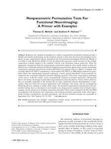
Page The horizontal component of the magnetic field measured in one minute resolution at Honolulu magnetic observatory from 1/1/2001 00:00 UT to 1/7/2001 24:00 UT. . . . . . . . . . . . . . . . . . . . . . . . . . .
8
Share prices of the Standard & Poor’s 100 index (SP) and the Exxon– Mobil Corporation (XOM). Dashed lines separate years. . . . . . . .
9
Intra-daily cumulative returns on 10 consecutive days for the Standard & Poor’s 100 index (SP) and the Exxon–Mobil Corporation (XOM). .
10
The horizontal component of the magnetic field measured in one minute resolution at Honolulu magnetic observatory from 1/1/2001 00:00 UT to 1/7/2001 24:00 UT. . . . . . . . . . . . . . . . . . . . . . . . . . .
14
Three weeks of centered time series of {Xn (ti )} derived from credit card transaction data. The vertical dotted lines separate days. . . . .
25
Two functional observations Xn derived from the credit card transactions (left–most panel) together with smooths obtained by projection on 40 and 80 Fourier basis functions. . . . . . . . . . . . . . . . . . .
25
Top: horizontal intensity (nT) measured at Honolulu 30/3/2001 13/4/2001 with the straight lines connecting first and last measurements in each day. Bottom: the same after subtracting the lines. . . .
27
Diagnostic plots of Chiou and M¨ uller (2007) for a synthetic data set simulated according to model (3.1.1) in which the errors εn follow the functional autoregressive model of Bosq (2000). . . . . . . . . . . . .
42
3.2
Magnetometer data on 10 consecutive days (separated by vertical dashed lines) recorded at College, Alaska (CMO) and Honolulu, Hawaii, (HON). 77
3.3
Magnetometer data on 10 chronologically arranged isolated substorm days recorded at College, Alaska (CMO), Honolulu, Hawaii, (HON) and Boulder, Colorado (BOU). . . . . . . . . . . . . . . . . . . . . .
79
Intra-daily cumulative returns on 10 consecutive days for the Standard & Poor’s 100 index (SP) and the Exxon–Mobil Corporation (XOM). .
82
3.4
xiii 3.5
Share prices of the Standard & Poor’s 100 index (SP) and the Exxon– Mobil Corporation (XOM). Dashed lines separate years. . . . . . . .
83
4.1
Daily temperatures in 1916 with monthly averages and functional object obtained by smoothing with B-splines. . . . . . . . . . . . . . . . 131
4.2 5.1
Graph of mean functions of last four segments. . . . . . . . . . . . . . 132 ¡ ¢ Estimated density of kδ n k22 kˆn∗ −k ∗ for the process obtained combining 0.05 BM and t n√n + BM . . . . . . . . . . . . . . . . . . . . . . . . . . . 155
5.2
¡ ¢ Estimated density of kδ n k22 kˆn∗ −k ∗ for the process obtained combining 0.45 BB and sin(t) n√n + BB. . . . . . . . . . . . . . . . . . . . . . . . . 156
CHAPTER 1 INTRODUCTION Functional data analysis (FDA) is a relatively new direction in statistics that refers to the analysis of data which consist of observed functions or curves recorded at a finite subset of some interval. Due to technological advances in measurement devices and increasing computational power, high frequency data is becoming an important subject of current statistical research. By high frequency data, we understand measurements or observations available on finite grid of points in am interval. One way to take this into account is to consider the data as an observation of the continuous random variable X(t), t ∈ T. A random variable X = {X(t), t ∈ T } takes values in an infinite dimensional space (or function space). An observation of X is referred to as a functional data point. While FDA and the multivariate data analysis share many common principles, the infinite-dimensional nature of the functional data presents many new challenges that are absent in the traditional multivariate analysis. On the other hand, traditional statistical methods often fail when we deal with functional data. One of the advantages of FDA over classical statistics is that the time points are not required to be equally spaced, they can vary from one subject to another. FDA does not assume that an observation at one time point in the interval is independent of that at another point within the same functional datum. It might be assumed to be independent from one functional datum to another, but not necessarily to be independent of observed values at distinct time points within the same functional datum. To clarify the notation, consider X(t) ∈ L2 [0, 1], i.e. we view a random curve
2 {X(t), t ∈ T } as a random element of L2 [0, 1] equipped with the Borel σ− algebra. Suppose the stochastic process {X(t), t ∈ T } is defined on a common probability space (Ω, F, P ). For fixed t ∈ T , X(t) is a measurable map from Ω to R. For fixed ω ∈ Ω, the function X(ω, ·) is a sample path of the stochastic process. For fixed ω a sample path X(ω, ·) is an equivalent class of functions that function space, for example L2 [0, 1] Hilbert function space. Since functions in the space L2 can be expressed in terms of basis functions generating the space and moreover since the space is separabile Hilbert space, each function in the space can be expressed as a countable linear combination of basis functions. Further explanation could be found in Lee (2004). Suppose {φk } is a set of basis functions of L2 , then for fixed ω there exist a unique sequence of numbers c1 , c2 , . . . ∈ l2 such that
(1.0.1)
X(t) =
∞ X
ck φk (t).
k=1
In (1.0.1) the stochastic process X(t, ω) is decomposed into two parts, namely ck and φk . Note that the randomness is reflected only in the coefficients ck = ck (ω). The typical FDA tends to include the following steps. Further details could be found in Ramsay (2005). • First of all, the raw data are collected, cleaned and organized. Functional observations are observed only at discrete sampling points values tj , and these may or may not be equally spaced. There may be replications of each function referred to as an observation Xi with different argument values tij . • The next step is to convert functional observations to functional form, i.e. the raw data for observation Xi are used to define a function Xi (t) that can be evaluated at all values of t over some interval. In order to do this a functional
3 basis should be chosen. A basis is a collection of basic functions whose linear combination defines the actual functional observation:
(1.0.2)
Xi (t) =
K X
cik φk (t), i = 1, . . . , N.
k=1
When basis functions φk (t) are specified, then the conversion of the data into functional data objects involves computing and storing the coefficients, cik of the expansion (1.0.2) into a coefficient matrix. It should be pointed out that this step usually involves dimension reduction and initial smoothing. Most commonly used bases include: – the Fourier basis: typically used for stable, periodic data, i.e. data without specific local features; – the B-spline or Wavelet basis: typically used for non-periodic data; – the exponential basis, a set of exponential functions, eλk t, each with a different rate parameter λk ; – the polynomial basis, consisting of the powers of t: 1, t, t2 , . . .; – the power basis, consisting of a sequence of possibly non-integer powers, including negative powers of an argument t that is usually required to be positive. • Next a variety of preliminary displays is performed and summary statistics are computed.
4 • The functions may also need to be registered or aligned in order to have important features found in each curve that occur at roughly the same argument values. • Exploratory analyses are carried out on the registered data. The main techniques include principal component analysis (PCA), canonycal correlation analysis (CCA), and principal differential analysis (PDA). • Models are constructed for the data. The models may be in the form of a functional linear model, functional time series model or in the form of a differential equation. • The models are evaluated using graphical checks, calculating various summary statistics and carrying formal tests of significance. For the last decade functional principal component (FPC) analysis has been the main tool to analyze the variability of functional data. As its classical counterpart, functional PCA is mainly used to identify a few orthogonal functions that most efficiently describe the variability of functional observations. The inherent complexity of functional data analysis, as a distinctly infinite-dimensional and infinite-parameter (or non parametric) problem, means that principal component methods assume a greater importance in FDA than in more traditional, finite dimensional settings. There is often no practical opportunity for estimating, in a meaningful way, the “distribution” of a random function. Both the representation of such a distribution, and the slow convergence rates of estimators, throw up obstacles which seem insurmountable in many cases. Considerations of this type indicate that the properties of the principal component functions are often going to be of greater importance than properties of the distribution itself. For example, it will be of greater interest to assess peaks and
5 troughs in a principal component function, than to look for extrema in the “density” of the distribution. The principal component functions appear explicitly in the Karhunen-Lo`eve representation of X(t), where they are weighted by scalar random variables. Further details could be found in Hall and Vial (2006). Functional variable can be a random surface or image, a vector of random curves or any other more complicated infinite dimensional mathematical object. Examples in which the collected data are curves arise in a variety of fields of applied sciences including environmetrics, chemometrics, biometrics, medicine, econometrics, physics, etc. To illustrate the notion of functional data we present a few data sets that motivated the research presented in this thesis. They are extensively analyzed in the dissertation. The currents flowing in the magnetosphere and ionosphere (M-I) form a complicated multiscale geosystem that contains the temporal scales from seconds to days. A magnetometer is an instrument that measures the three components of the magnetic field at a location where it is placed. There are over 100 magnetic observatories located on the surface of the Earth, and most of them have digital magnetometers. These magnetometers record the strength and direction of the field every five seconds, but the magnetic field exists at any moment of time, so it is natural to think of a magnetogram as an approximation to a continuous record. The raw magnetometer data are cleaned and reported as averages over one minute intervals. Such averages were used to produce Figure 1.1. Thus 7 ×24×60 = 10, 080 values (of one component of the field) were used to draw Figure 1.1. The dotted vertical lines separate days in Universal Time (UT). It is natural to view a curve defined over one UT day as a single observation because one of the main sources influencing the shape of the record is the daily rotation of the Earth. When an observatory faces the Sun, it records the magnetic field generated by wind currents flowing in the ionosphere which are
6 driven mostly by solar heating. Thus, Figure 1.1 shows seven consecutive functional observations. In contrast to the magnetic field, the price of an asset exists only when the asset is traded. A great deal of financial research has been done using the closing daily price, i.e. the price in the last transaction of a trading day. However many assets are traded so frequently that one can practically think of a price curve that is defined at any moment of time. Intra–daily prices of financial instruments are well-known to have properties quite different than those of daily or monthly closing prices and also offer new interesting research perspectives. It is natural to choose one trading day as the underlying time interval. To illustrate, consider the S&P 100 index and its major component, the Exxon Mobil Corporation (currently it contributes 6.78% to this index). The price processes over the period of about 8 years are shown in Figure 1.2. For these data, Pn (tj ) is the price on day n at tick tj (time of trade). For such data, it is not appropriate to define returns by looking at price movements between the ticks because that would lead to very noisy trajectories for FDA methods, based on the FPC’s, are not appropriate; Johnstone and Lu (2009) explain why principal components cannot be meaningfully estimated for such data. Instead, we adopt the following definition of the intra-daily cumulative returns. Suppose Pn (tj ), n = 1, . . . , N, j = 1, . . . , m, is the price of a financial asses at time tj on day n. We call the functions
rn (tj ) = 100[ln Pn (tj ) − ln Pn (t1 )], j = 2, . . . , m, n = 1, . . . , N,
the intra-daily cumulative returns. Figure 1.3 shows intra-daily cumulative returns on 10 consecutive days for the Standard & Poor’s 100 index and the Exxon Mobil Corporation. These returns have now an appearance amenable to smoothing via
7 FPC’s. The dissertation consists of several chapters, which represent individual manuscripts on goodness of fit and change point tests for functional observations. Chapter 2 introduces a test for independence and identical distribution of functional observations. Two inferential tests for error correlation in the functional linear model are put forward in Chapter 3. Chapter 4 deals with the novel test for detecting a change point in the mean of functional observations, while Chapter 5 develops and discusses a comprehensive asymptotic theory for the estimation of a change–point in the mean function of functional observations.
27560
27580
27600
27620
27640
27660
8
0
2000
4000
6000
8000
10000
Time
Fig. 1.1: The horizontal component of the magnetic field measured in one minute resolution at Honolulu magnetic observatory from 1/1/2001 00:00 UT to 1/7/2001 24:00 UT.
9
Fig. 1.2: Share prices of the Standard & Poor’s 100 index (SP) and the Exxon–Mobil Corporation (XOM). Dashed lines separate years.
0.5 0.0 −1.5 −1.0 −0.5
SP returns
1.0
1.5
10
0
1000
2000
3000
4000
1.0 0.5 −0.5 0.0
XOM returns
1.5
2.0
min
0
1000
2000
3000
4000
min
Fig. 1.3: Intra-daily cumulative returns on 10 consecutive days for the Standard & Poor’s 100 index (SP) and the Exxon–Mobil Corporation (XOM).
11
CHAPTER 2 PORTMANTEAU TEST OF INDEPENDENCE FOR FUNCTIONAL OBSERVATIONS1
2.1
Introduction The last two decades have seen the emergence of new technology allowing the
collection and storage of time series of finely sampled observations. Every single trade on a speculative asset is recorded and stored, and so e.g. minute by minute values of an asset are available, resulting in 390 observations in a six and half hour trading day rather than one closing price. Similar examples abound. Data of this type can be conveniently viewed as functional observations, e.g. we treat the curve built up of 390 minute by minute values of an asset as a one single observation. Most inferential tools of Functional Data Analysis, see Ramsay and Silverman (2005), rely on the assumption of iid functional observations. In designed experiments (see e.g. M¨ uller and Stadtm¨ uller (2005), this assumption can be ensured, but in observational data derived from time series it requires a verification. In traditional (nonfunctional) time series analysis, tests of independence and residual–based diagnostic tests derived from them play a fundamental role. In this paper we propose a simple portmanteau test of independence for functional observations. In addition to its direct applicability, this test, with the underlying theory and numerical work presented here, will likely form the basis for residual–based specification tests for various functional time series models. While there are many such tests for real– and vector– valued observations, see Hosking (1980) and Li (1981) among others, no methodology is yet available for functional data. 1
COAUTHORED BY R. GABRYS, AND P. KOKOSZKA. REPRODUCED BY PERMISSION FROM JOURNAL OF THE AMERICAN STATISTICAL ASSOCIATION, VOL. 102, NO. 480, PAGES 1338–1348, 2007.
12 The idea of the test is simple and intuitively appealing. The functional observations Xn (t), t ∈ [0, T ), n = 1, 2, . . . , N, are approximated by the first p terms of the principal component expansion
(2.1.1)
Xn (t) ≈
p X
Xkn vk (t),
n = 1, 2, . . . , N.
k=1
The vk (t) are the principal modes of variation (principal components, PC’s), and the Xkn are the random weights (scores) corresponding to each individual curve. Viewing, for the sake of an intuitive argument, the vk (t) as deterministic curves, the iid assumption for the curves Xn (·) implies this assumption for the random vectors [X1n , . . . , Xpn ]0 . To test it, the method proposed by Chitturi (1976) can be used. In reality, the vk (t) must be replaced by estimated PC’s. This transition is not trivial because the estimated PC’s depend on all observations. Moreover, the difference between the population and sample PC’s is of the order N −1/2 , and so the limit distribution of some statistics may contain an extra term. Our test statistic is based on products of scores, and we show that the effect of estimation of the PC’s is asymptotically negligible. We also show by simulations that it has a small effect on the finite sample performance of the test. An example of data which motivated this research is shown in Figure 2.1. About a hundred terrestrial geomagnetic observatories form a network, INTERMAGNET, designed to monitor and understand the behavior of currents of charged particles flowing in the magnetosphere and ionosphere. Modern digital magnetometers record three components of the magnetic field in five second resolution, but the data available at INTERMAGNET’s website (http://www.intermagnet.org) or CD’s consist of one minute averages (1440 data points per day per component per observatory). The recent availability of these large data sets may lead to new insights if appropriate statistical tools are developed. In this respect, Functional Data Analysis stands out with its unique strength: physicists naturally view magnetogram records as curves
13 reflecting a continuous change in the structure of the various magnetic fields. In Figure 2.1, the daily variation caused by the rotation of the Earth is prominent. Notice however that the periodic pattern is not strong, as the current system is often nonlinearly disturbed by solar energy flows. For this reason, tools of traditional time series analysis based on stationarity, seasonality and polynomial trends are not suitable. The paper is organized as follows. In Section 2.2, we formulate the test procedure together with mathematical assumptions and theorems establishing its asymptotic validity. The proofs of the theorems of Section 2.2 are presented in Section 2.5. Sections 4.4 and 2.4 are devoted, correspondingly, to the study of the finite sample performance of the test and its application to two types of functional data: credit card sales and geomagnetic records. Section 2.6 contains some lemmas on Hilbert space valued random elements which are used in Section 2.5, and may be useful in other similar contexts. In Section 2.7, we develop the required theory for random matrices.
2.2
Assumptions and main results We first state the assumptions and introduce some notation. Our main result
establishing limit null distribution is stated in Theorem 2.1. The consistency against the popular functional AR(1) model is established in Theorem 2.2. We observe random functions {Xn (t), t ∈ [0, 1), n = 1, 2, . . . N } and want to test H0 : the Xn (·) are independent and identically distributed versus HA : H0 does not hold. We assume that the Xn are measurable elements of the space L2 [0, 1) in which R1 the norm is defined by ||X||2 = 0 X 2 (t)dt.
27560
27580
27600
27620
27640
27660
14
0
2000
4000
6000
8000
10000
Time
Fig. 2.1: The horizontal component of the magnetic field measured in one minute resolution at Honolulu magnetic observatory from 1/1/2001 00:00 UT to 1/7/2001 24:00 UT.
15 For theoretical convenience we assume that the Xn have mean zero. We explain in Section 2.4 how to center the data. Our theory is valid under the assumption of finite fourth moments: ·Z (2.2.2)
1
4
E||Xn || = E 0
¸2 Xn2 (t)dt
< ∞.
If the Xn form a strictly stationary sequence (as is the case under H0 ), we denote by X a random element with the distribution of the Xn and define the covariance operator C(x) = E[hX, xi X], x ∈ L2 [0, 1). The empirical covariance operator is defined by N 1 X hXn , xi Xn , x ∈ L2 [0, 1). CN (x) = N n=1
The eigenelements of C are defined by C(vj ) = λj vj , j ≥ 1. The eigenfunctions vj form an orthonormal basis of L2 [0, 1). We assume λ1 ≥ λ2 ≥ λ3 , . . . . The empirical eigenelements are defined by CN (vjN ) = λjN vjN , j = 1, 2, . . . N. where we assume λ1N ≥ λ2N ≥ . . . ≥ λN N . Since the operators C and CN are symmetric and nonnegative definite, the eigenvalues λj and λjN are nonnegative.
16 If the eigenspace corresponding to the eigenvalue λk is one dimensional, then formula (4.49) on p. 106 of Bosq (2000) implies that lim sup N E||vk − vkN ||2 < ∞.
(2.2.3)
N →∞
(Note that n before the expected value is missing in formula (4.49) of Bosq (2000), cf. formulas (4.17) and (4.44) of that monograph.) To establish the null distribution of the test statistic QFN defined below, we merely require the following assumption: Assumption 2.2.
The functional observations Xn are mean zero in L2 [0, 1), and
(2.2.2) and (3.2.3) for k ≤ p hold. The number p (of principal components) appears in the statements of our main results. We approximate the Xn (t) by XnF (t)
=
p X
F Xkn vkN (t),
k=1
where Z (2.2.4)
F Xkn
1
:= 0
Z XnF (t)vkN (t)dt
1
=
Xn (t)vkN (t)dt. 0
The Xn (t) are thus the projections of the functional observations on the subspace spanned by the largest p empirical principal components, see Chapter 8 of Ramsay and Silverman (2005). We will work with the random vectors (2.2.5)
F 0 F F ]. , . . . , Xpn , X2n XFn = [X1n
17 and analogously defined (unobservable) vectors Xn = [X1n , X2n , . . . , Xpn ]0 ,
(2.2.6) where
Z (2.2.7)
1
Xkn =
Xn (t)vk (t)dt. 0
Under H0 , the Xn are iid mean zero random vectors in Rp for which we denote v(i, j) = E[Xit Xjt ],
V = [v(i, j)]i,j=1,...,p .
The matrix V is thus the p × p covariance matrix. By Ch we denote the sample autocovariance matrix whose entries are N −h 1 X ch (k, l) = Xkt Xl,t+h , N t=1
0 ≤ h < N.
−1 Denote by rf,h (i, j) and rb,h (i, j) the (i, j) entries of C−1 0 Ch and Ch C0 , respectively
and introduce the statistic (2.2.8)
QN = N
p H X X
rf,h (i, j)rb,h (i, j).
h=1 i,j=1
d
Theorem 2.11 shows that under H0 , QN → χ2p2 H . Analogously to the way the statistic QN (2.2.8) is constructed from the vectors Xn , n = 1, . . . , N , we construct the statistic QFN from the vectors XFn , n = 1, . . . , N . The following theorem establishes the limit null distribution of the test statistic QFN . d
Theorem 2.1. Under H0 , if Assumption 2.2 holds, then QFN → χ2p2 H .
18 Theorem 2.1 is proven in Section 2.5. Out of many possible directional alternatives, we focus on the ARH(1) (H stands for Hilbert Space) model of Bosq (2000) which has been used in several interesting applications [see e.g. Laukaitis and Raˇckauskas (2002), Fern´andez de Castro et al. (2005) and Kargin and Onatski (2008)]. It introduces serial correlation analogous to the usual AR(1) model. Suppose then that (2.2.9)
Xn+1 = ΨXn + εn
with iid mean zero innovations εn ∈ L2 [0, 1). We assume that the operator Ψ is bounded, the solution to equations (2.2.9) is stationary and Assumption 2.2 holds. These conditions are implied by very mild assumptions on Ψ, see Chapters 3 and 4 of Bosq (2000). It is easy to check that the vectors (2.2.6) form a stationary VAR(1) process:
Xk,n+1 =
p X
ψki Xin + εk,n+1 ,
k = 1, 2, . . . , p,
i=1
where ψik = hvi , Ψvk i , εk,n = hεn , vk i . In the vector form (2.2.10)
Xn+1 = ΨXn + en+1 .
If the operator Ψ is not zero, there are i, k ≥ 1 such that ψik 6= 0. The following theorem establishes the consistency against the ARH(1) model (2.2.9). Theorem 2.2. Suppose the functional observations Xn follow a stationary solution to equations (2.2.9), Assumption 2.2 holds, and p is so large that the p × p matrix Ψ P
in (2.2.10) is not zero. Then QFN → ∞.
19 Table 2.1: Empirical size (in percent) of the test using Fourier basis. The simulated observations are Brownian bridges. Lag
p=3 10% 5%
1%
1 3 5
7.7 6.8 4.9
2.5 2.5 2.0
0.6 0.3 0.0
1 3 5
9.0 8.1 8.8
5.1 3.5 3.6
0.4 0.6 0.6
1 3 5
9.8 9.3 7.2
4.6 4.8 3.7
1.2 1.0 1.0
p=4 10% 5% N=50 7.4 2.8 6.7 3.3 3.6 1.4 N=100 8.9 3.9 8.3 4.0 6.6 2.7 N=300 9.4 4.0 9.1 4.7 8.2 3.8
1%
p=5 10% 5%
1%
0.3 0.6 0.2
7.9 4.9 4.0
3.5 2.0 1.7
0.4 0.3 0.2
0.6 0.9 0.3
10.0 7.5 6.7
3.9 3.2 2.4
0.8 0.4 0.3
0.9 0.9 0.7
10.1 10.0 10.6
4.7 5.4 5.5
0.6 0.8 1.2
Theorem 2.2 is proven in Section 2.5. Other departures from the null can be treated in a similar manner. The idea is that under the null the sample autocoF variances of the Xkn at a positive lag converge in distribution when multiplied by √ N , whereas under any reasonable alternative, these autocovariances tend in prob-
ability to some constants. This could be used to establish consistency against local alternatives, but this theoretical investigation is not pursued here.
2.3
Finite sample performance In this section we investigate the finite sample properties of the test using some
generic models and sample sizes typical of applications discussed in Section 2.4. To investigate the empirical size, we generated independent trajectories of the standard Brownian motion (BM) on [0, 1] and the standard Brownian bridge (BB). This was done by transforming cumulative sums of independent normal variables computed on a grid of m equispaced points in [0, 1]. We used values of m ranging from 10 to 1440, and found that the empirical size basically does not depend on m
20 (the tables of this section use m = 100). To compute the principal components vkN and the corresponding eigenvalues using the R package fda, the functional data must be represented (smoothed) using a specified number of functions from a basis. We worked with Fourier and B splines functional bases and used 8, 16, and 80 basis functions. All results are based on one thousand replications. Table 2.1 shows empirical sizes for the Brownian bridge and and the Fourier basis for several values of the lag H = 1, 3, 5, the number of principal components p = 16, 80 and sample sizes N = 50, 100, 300. The standard errors in this table are between 0.5 and 1 percent. In most cases,the empirical sizes are within two standard errors of the nominal size, and the size improves somewhat with increasing N . The same is true for the BM and B splines; no systematic dependence on the type of data or basis is seen, which accords with the nonparametric nature of the test. Of course, since the CLT is used to establish the asymptotic validity of the test, results are likely to be worse for nonnormal data, but a detailed empirical study is beyond the intended scope of this paper. In a power study, we focus on the ARH(1) model (2.2.9), which can be more explicitly written as: Z (2.3.11)
1
Xn (t) =
ψ(t, s)Xn−1 (s)ds + εn (t),
t ∈ [0, 1],
n = 1, 2, . . . , N.
0
A sufficient condition for the assumptions of Theorem 2.2 to hold is Z (2.3.12)
1
2
Z
1
||Ψ|| = 0
ψ 2 (t, s)dtds < 1.
0
The norm in (2.3.12) is the Hilbert–Schmidt norm.
21 Table 2.2: Empirical power of the test using Fourier basis. The observations follow the ARH(1) model (2.3.11) with Gaussian kernel with ||Ψ|| = 0.5 and iid standard Brownian motion innovations. Lag
p=3 10% 5%
1%
1 3 5
44.7 35.2 26.7
33.8 17.7 27.0 13.3 20.0 11.0
1 3 5
71.2 67.9 62.3
64.2 51.4 61.0 44.9 54.6 38.6
1 3 5
98.7 97.6 96.8
98.2 96.7 97.1 95.5 95.9 92.8
p=4 10% 5% N=50 41.9 29.4 34.0 24.7 24.4 15.8 N=100 74.4 66.5 67.5 58.6 59.0 49.9 N=300 99.2 98.9 99.0 98.4 98.1 97.0
1%
p=5 10% 5%
1%
12.6 10.8 8.1
38.5 26.1 33.2 21.6 21.5 14.3
9.2 8.7 6.0
48.1 42.8 32.3
77.7 68.0 68.4 56.9 55.1 45.5
46.1 38.1 27.9
97.2 96.8 93.8
99.8 99.5 99.2 98.3 98.4 97.3
98.5 96.6 94.4
In our study, the innovations εn in (2.3.11) are either standard BM’s or BB’s. We used two kernel functions: the Gaussian kernel ½ ψ(t, s) = C exp
t2 + s2 2
¾ , (t, s) ∈ [0, 1]2 ,
and Wiener kernel ψ(t, s) = C min(s, t), (t, s) ∈ [0, 1]2 . The constants C were chosen so that ||Ψ|| = 0.3, 0.5, 0.7. We used both Fourier and B spline basis. The power against this alternative is expected to increase rapidly with N , as the test statistic is proportional to N . This is clearly seen in Table 2.2. The power also increases with ||Ψ||; for ||Ψ|| = 0.7 and the Gaussian kernel, it is practically 100% for N = 100 and all choices of other parameters. There are two less trivial observations. The power is highest for lag H = 1.
22 Table 2.3: Empirical power of the test using Fourier basis. The observations follow the ARH(1) model (2.3.11) with Gaussian kernel with ||Ψ|| = 0.5 and iid standard Brownian bridge innovations. Lag 10%
p=3 5%
1 3 5
98.3 95.2 86.9
97.0 92.1 90.3 77.4 80.2 61.7
1 3 5
100 100 99.9
100 100 100 99.9 99.3 98.7
1 3 5
100 100 100
100 100 100
1%
100 100 100
p=4 10% 5% N=50 98.4 96.4 92.1 86.2 78.5 71.7 N=100 100 100 100 100 99.9 99.8 N=300 100 100 100 100 100 100
p=5 5%
1%
87.6 69.6 51.4
99.1 97.3 89.9 85.1 75.2 63.9
87.6 63.2 40.4
100 99.7 98.6
100 100 100 99.9 99.7 99.5
100 99.8 97.8
100 100 100
100 100 100
100 100 100
1%
10%
100 100 100
This is because for the ARH(1) process the “correlation” between Xn and Xn−1 is largest at this lag. By increasing the maximum lag H, the value of QFN generally increases, but the critical value increases too (df increases by p2 for a unit increase in H). The power also depends on how the action of the operator Ψ is “aligned” with the eigenfunctions vk . If the inner products hvi , Ψvk i are large in absolute value, the power is high. Thus, with all other parameters being the same, the power in Table 2.3 is greater than in Table 2.2 because of the different covariance structure of the Brownian bridge and the Brownian motion. In all cases, the power for the Wiener kernel is slightly lower than for the Gaussian kernel. A full set of size and power tables is available upon request. The empirical sizes for the two processes we simulated are generally fairly close to nominal sizes and are not much affected by the choice of H and p. Power against the ARH(1) model is very good if H = 1 is used.
23 2.4
Application to credit card transactions and diurnal geomagnetic variation In this section, we apply our test to two data sets which naturally lend themselves
to functional data analysis. The first data set, studied in Laukaitis and Raˇckauskas (2002), consists of the number of transactions with credit cards issued by Vilnius Bank, Lithuania. The second, is a daily geomagnetic variation, a similar data set was studied by Xu and Kamide (2004). Suppose Dn (ti ) is the number of credit card transactions in day n, n = 1, . . . , 200, (03/11/2000 – 10/02/2001) between times ti−1 and ti , where ti − ti−1 = 8 min, i = 1, . . . , 128. For our analysis, the transactions were normalized to have time stamps in interval [0, 1], which thus corresponds to one day. To remove the weekly periodicity, we work with the differences Xn (ti ) = Dn (ti ) − Dn−7 (ti ), n = 1, 2, . . . , 193. Figure 2.2 displays the first three weeks of these data. A characteristic pattern of an AR(1) process with clusters of positive and negative observations is clearly seen. Two consecutive days are shown in the left–most panel of Figure 2.3 together with functional objects obtained by smoothing with 40 and 80 Fourier basis functions. As expected, the test rejects the null hypothesis at 1% level for both smooths, and all lag values 1 ≤ H ≤ 5 and the number of principal components equal to 4, 5, 10 and 20. We estimated the ARH(1) model (2.3.11) using the function linmod from the R package fda, see Malfait and Ramsay (2003) and Ramsay and Silverman (2002, 2005). Table 2.4 displays the P-values which support this model choice, see Laukaitis and Raˇckauskas (2002). Note how starting with p = 2 or p = 3 the P-values increase and approach 100%. This accords with the findings of Section 4.4, and is caused by the fact that the dependence is captured by only a few most important principal components, and increasing p does not change the sampling distribution of QFN very much, but shifts the limiting distribution to the right. We note that, in analogy with well–known results for real–valued time series, see e.g. Ljung and Box (1978) and references therein, the number of degrees of freedom in the asymptotic distribution
24 Table 2.4: P-values for the functional ARH(1) residuals of the credit card data Xn . Lag, H
p=1
p=2
1 2 3
69.54 22.03 35.57 38.28 54.44 53.63
1 2 3
57.42 18.35 35.97 23.25 36.16 36.02
p=3 p=4 BF=40 13.60 46.29 7.75 47.16 25.28 52.61 BF=80 53.30 89.90 23.83 45.07 26.79 30.21
p=5
p=6
p=7
80.35 64.92 71.33
96.70 99.20 95.00 99.04 86.84 94.93
88.33 55.79 56.81
95.40 99.19 46.39 70.65 34.51 47.00
of the statistic QFN computed from residuals of the ARH(1) model is likely to be less than p2 H. This question is a subject of on–going research, but even with this caveat, Table 2.4 gives strong support to the ARH(1) model. We now turn to the ground-based magnetogram records which reflect the variations of the currents flowing in the Magnetosphere/Ionosphere. These data are used to understand the structure of this important complex geosystem. Since we present here merely an illustration of our procedure, we focus only on the horizontal intensity measured at Honolulu in 2001. The horizontal (H) intensity is the component of the magnetic field tangent to the Earth’s surface and pointing toward the magnetic North; its variation best reflects the changes in the large currents flowing in the magnetic equatorial plane. The top panel of Figure 2.4 shows two weeks of these data. Xu and Kamide (2004) used the H–component measured at Beijing in 2001 in order to understand the statistical structure of the daily variation and associate it with known or conjectured currents. Following Xu and Kamide (2004), we subtracted the linear change over a day to obtain the curves like those showed in the bottom panel of Figure 2.4. After centering over a period under study, we obtain the functional observations we work with. The analysis was conducted using Fourier base functions.
−200
−100
0
100
200
300
400
25
0
500
1000
1500
2000
2500
3000
Time
200
−50
0
0
0
50
50
50
100
100
100
150
150
150
200
Fig. 2.2: Three weeks of centered time series of {Xn (ti )} derived from credit card transaction data. The vertical dotted lines separate days.
20
40
60
80
100
0
20
40
60
80
100
0.0
0.2
0.4
0.6
0.8
1.0
0.0
0.2
0.4
0.6
0.8
1.0
0.0
0.2
0.4
0.6
0.8
1.0
0.0
0.2
0.4
0.6
0.8
1.0
−20
0
0
0
20
20
20
40
40
40
60
60
60
80
80
100
80
100
120
0
Fig. 2.3: Two functional observations Xn derived from the credit card transactions (left–most panel) together with smooths obtained by projection on 40 and 80 Fourier basis functions.
26 We note that the issue of separating the daily variation from larger disturbances caused by magnetic storms is a complex one, and is the subject of on–going geophysical research, see Jach et al. (2006) for a recent contribution. For example, one can question whether what we see in the second day in the bottom panel of Figure 2.4 is an unusually large daily variation or an unremoved signature of a magnetic storm. This paper is however not concerned with such issues. Testing one year magnetometer data with lags H = 1, 2, 3 and different numbers of principal components p = 3, 4, 5, yields P–values very close to zero. This indicates that while principal component analysis, advocated by Xu and Kamide (2004), may be a useful exploratory tool to study daily variation over the whole year, one must be careful when using any inferential tools based on it, as they typically require a simple random sample, see e.g. Section 5.2 of Seber (1984). We also applied the test to smaller subsets of data roughly corresponding to boreal Spring and Summer. The P–values reported in Table 2.5 show that the transformed data can to a reasonable approximation be viewed as a functional simple random sample. The discrepancy in the outcome of the test when applied to the whole year and to a season is probably due to the annual change of the position of the Honolulu observatory relative to the Sun whose energy drives the convective currents mainly responsible for the daily variation. The two examples discussed in this section show that our test can detect departures from the assumption of independence (credit card data) or from the assumption of identical distribution (magnetometer data), and confirm both assumptions when they are expected to hold. In our examples, the results of the test do not depend much on the choice of the functional basis.
27 Table 2.5: P-values for the magnetometer data split by season. Feb, Mar, Apr, May p=4 p=5 13.44 6.51 3.37 2.99
Jun, Jul, Aug, Sep p=4 p=5 1.03 1.23 31.72 42.59
27200
27400
27600
Lag H 1 3
0
200
400
600
800
1000
1200
1400
800
1000
1200
1400
−400
−200
0 100 200
Time
0
200
400
600 Time
Fig. 2.4: Top: horizontal intensity (nT) measured at Honolulu 30/3/2001 - 13/4/2001 with the straight lines connecting first and last measurements in each day. Bottom: the same after subtracting the lines.
28 2.5
Proofs of Theorems 2.1 and 2.2 P
Proof of Theorem 2.1. By Theorem 2.11, it is enough to show that QFN − QN → 0. By (2.2.8), this will follow if we show that for h ≥ 1 P
N 1/2 (CFh − Ch ) → 0
(2.5.13) P
and CF0 − C0 → 0. We will verify that (2.5.13) holds for all h ≥ 0. Recall that
ch (k, l) =
N −h 1 X Xkn Xl,n+h ; N n=1
cFh (k, l) =
N −h 1 X F F . X X N n=1 kn l,n+h
Therefore cFh (k, l) − ch (k, l) = M1 + M2 , where N −h 1 X F M1 = (Xkn − Xkn )Xl,n+h ; N n=1
N −h 1 X F F M2 = X (Xl,n+h − Xl,n+h ). N n=1 kn
P
We will first show that N 1/2 M1 → 0. Observe that N 1/2 M1 = N −1/2
N −h X
hXn , vk − vkN i hXn+h , vl i
n=1
* =
N −1/2
N −h X
+ hXn+h , vl i Xn , vk − vkN
= hSN , YN i ,
n=1
where SN := N
−1/2
N −h X
hXn+h , vl i Xn ;
YN = vk − vkN
n=1
Note that by (3.2.3), E| hSN , YN i | ≤ E[||SN || ||YN ||] ≤ (E||SN ||2 )1/2 (E||YN ||2 )1/2 = O(N −1/2 )(E||SN ||2 )1/2 .
29 P
To show that N 1/2 M1 → 0, it thus remains to verify that E||SN ||2 is bounded. Notice that E||SN ||2 = N −1 E||
N −h X
hXn+h , vl i Xn ||2
n=1
= N −1 E
N −h X
hXm+h , vl i hXn+h , vl i hXm , Xn i
m,n=1
=N
−1
N −h X
£ ¤2 E[hXn+h , vl i]2 E||Xn ||2 ≤ E||Xn ||2 .
n=1 P
To show that N 1/2 M2 → 0, decompose M2 as M2 = M21 + M22 , where
M21
M22
N −h 1 X = hXn , vk i hXn+h , vl − vlN i ; N n=1
N −h 1 X = hXn , vkN − vk i hXn+h , vl − vlN i . N n=1 P
P
By the argument developed for M1 , N 1/2 M21 → 0, so we must show N 1/2 M22 → 0. This follows from Lemma 2.7. Proof of Theorem 2.2. We first state Lemmas 2.3 and 2.4 which form two critical building blocks of the proof. Lemma 2.3. Suppose the vectors Xn = [X1n , X2n , . . . , Xpn ]0 follow a stationary vector AR(1) process Xn+1 = ΨXn + en+1 . The errors en are iid mean zero with finite variance and en+1 is independent of Xn . Then, p X
P
rf,1 (i, j)rb,1 (i, j) → tr[ΨVΨ0 V−1 ],
i,j=1
where V is the covariance matrix of the vector Xn .
30 Proof. Observe that N −1 N −1 1 X 1 X 0 C1 = Xn Xn+1 = Xn [ΨXn + en+1 ]0 N n=1 N n=1
N N −1 1 X 1 X 0 0 = Xn Xn Ψ + oP (1) + Xn e0n+1 = VΨ0 + oP (1), N n=1 N n=1
by the ergodic theorem. Consequently, P
0 C−1 0 C1 → Ψ ;
P
P
0 −1 C1 C−1 0 → VΨ V
P
and so rf,1 (i, j) → ψji and rb,1 (i, j) → [VΨ0 V−1 ]ij . Therefore p X
P
rf,1 (i, j)rb,1 (i, j) →
i,j=1
p p X X
ψji [VΨ0 V−1 ]ij =
j=1 i=1
p X
[ΨVΨ0 V−1 ]jj = tr[ΨVΨ0 V−1 ].
j=1
Lemma 2.4. If V is a symmetric positive definite p × p matrix and Ψ is a nonzero matrix of the same dimension, then tr[ΨVΨ0 V−1 ] > 0. Proof. To get a feel why this result is true, suppose p = 2 and V is diagonal, i.e.
λ1 0 V= , 0 λ2 Then
ψ11 ψ12 Ψ= . ψ21 ψ22
ψ11 λ−1 1
ψ21 λ−1 2
ψ11 λ1 ψ12 λ2 ΨVΨ0 V−1 = −1 −1 ψ12 λ1 ψ22 λ2 ψ21 λ1 ψ22 λ2
=
2 ψ11
+
2 λ2 λ−1 ψ12 1
ψ21 ψ11 + ψ22 ψ12 λ2 λ−1 1
ψ11 ψ21 λ1 λ−1 2
+ ψ12 ψ22 . 2 2 + ψ λ1 λ−1 ψ21 2 22
Since λ1 and λ2 are positive, the trace is positive if one of the ψjk is positive.
31 For arbitrary symmetric positive definite V, there is an orthonormal matrix P such that V = PΛP0 , where Λ is diagonal, and its diagonal consists of positive eigenvalues of V. Therefore ΨVΨ0 V−1 = ΨPΛP0 Ψ0 (PΛP0 )−1 = ΨPΛP0 Ψ0 PΛ−1 P0 . Since tr(AB) = tr(BA), setting A = ΨPΛP0 Ψ0 PΛ−1 and B = P0 , we obtain tr[ΨVΨ0 V−1 ] = tr[P0 ΨPΛP0 Ψ0 PΛ−1 ] = tr[ΦΛΦ0 Λ−1 ], where Φ = P0 ΨP. Since Ψ = PΦP0 , Φ is nonzero. Direct verification shows that P the jth diagonal entry of ΦVΦ0 V−1 is pk=1 φ2jk λk λ−1 j , and so 0
(2.5.14)
−1
tr[ΨVΨ V ] =
p p X X
φ2jk λk λ−1 j > 0.
j=1 k=1
Lemma 2.5. If V is a symmetric nonnegative definite p × p matrix and Ψ is any matrix of the same dimension, then tr[ΨVΨ0 V] ≥ 0. Proof.Proceeding exactly as in the proof of Lemma 2.4, we obtain 0
tr[ΨVΨ V] =
p p X X
φ2jk λk λj ≥ 0.
j=1 k=1
We now present the remainder of the proof of Theorem 2.2. Direct verification shows that (2.5.15)
p X i,j=1
© ª F F rf,h (i, j)rb,h (i, j) = tr [CFh ]0 [CF0 ]−1 CFh [CF0 ]−1 .
32 If [CF0 ]−1 exists, it is positive definite, so by (2.5.14) and Lemma 2.5, p X
F F rf,h (i, j)rb,h (i, j) ≥ 0.
i,j=1
By Lemmas 2.3 and 2.4, p X
P
rf,1 (i, j)rb,1 (i, j) → q > 0.
i,j=1
It thus suffices to show that p X £
(2.5.16)
¤ P F F rf,1 (i, j)rb,1 (i, j) − rf,1 (i, j)rb,1 (i, j) → 0.
i,j=1
P
Relation (2.5.16) will follow from CFh − Ch → 0. In the remainder of the proof we use the notation introduced in the proof of P
P
Theorem 2.1. We must show that M1 → 0 and M2 → 0. We will display the argument only for M1 . Observe that * M1 =
N −1
N −h X
+ hXn+h , vl i Xn , vk − vkN
n=1
P
By (3.2.3), ||vk − vkN || → 0. Since,
E||N
−1
N −h X n=1
P
it follows that M1 → 0.
hXn+h , vl i Xn || ≤ E|| hXn+h , vl i Xn || ≤ E||Xn ||2 ,
33 2.6
Auxiliary Lemmas for H-valued random elements Consider the empirical lag-h autocovariance operator N −h 1 X CN,h (x) = hXn , xi Xn+h . N n=1
(2.6.17)
Recall that the Hilbert-Schmidt norm of a Hilbert-Schmidt operator S is defined by ∞ X
||S||2S =
||S(ej )||2 ,
j=1
where {e1 , e2 , . . .} is any orthonormal basis. Lemma 2.6. Suppose the Xi are iid random elements in a separable Hilbert space with E||X0 ||2 < ∞, then E||CN,h ||2S =
¢ N −h¡ 2 2 E||X || . 0 N2
Proof. Observe that ||CN,h ||2S
=
∞ X
||CN,h (ej )||2
j=1
=
∞ X
*
j=1
N −h N −h 1 X 1 X hXn , ej i Xn+h , hXm , ej i Xm+h N n=1 N m=1
+
∞ N −h X 1 X = hXm , ej i hXn , ej i hXm+h , Xn+h i . N 2 m,n=1 j=1
It follows from the independence of the Xn that E||CN,h ||2S
N −h ∞ 1 XX = 2 E[hXn , ej i]2 E[hXn+h , Xn+h i]2 N n=1 j=1
"∞ # N −h X ¤2 N − h £ 1 X 2 . E = E||X0 || 2 [hXn , ej i] = E||X0 ||2 N n=1 N2 j=1 2
34 Lemma 2.7. Suppose Xn , ZN , YN are random elements in a separable Hilbert space. We assume E||YN ||2 = O(N −1 ),
(2.6.18)
(2.6.19)
Xn ∼ iid,
Then N −1/2
N −h X
E||ZN ||2 = O(N −1 );
E||Xn ||2 < ∞.
P
hXn , YN i hXn+h , ZN i → 0.
n=1
Proof. Observe that N −1/2
N −h X
® hXn , YN i hXn+h , ZN i = CN,h (YN ), N 1/2 ZN ,
n=1
with the operator CN,h defined in (3.9.34). Since P (N 1/2 ||ZN || > C) ≤ C −2 N E||ZN |2 , P
N 1/2 ||ZN || = OP (1). Thus it remains to verify that CN,h (YN ) → 0. Since the Hilbert– Schmidt norm is not less than the uniform operator norm || · ||L , see Bosq (2000), p. 35, we obtain from Lemma 2.6: E||CN,h (YN )|| ≤ E[||CN,h ||L ||YN ||] ≤ E[||CN,h ||S ||YN ||] ¡ ¢1/2 ¡ ¢1/2 ≤ E||CN,h ||2S E||YN ||2 = O(N −1/2 )O(N −1/2 ) = O(N −1 ).
2.7
Limit theory for sample autocovariance matrices Detailed proofs of Theorems 2.8, 2.10, 2.11, Remark 2.9 and all displayed for-
mulas leading to them are omitted to conserve space, but are available upon request. Consider random vectors X1 , . . . , XN , where Xt = [X1t , X2t , . . . , Xpt ]0 . We assume
35 that the Xt , t = 1, 2, . . . are iid mean zero with finite variance and denote v(i, j) = E[Xit Xjt ],
V = [v(i, j)]i,j=1,...,p .
By Ch we denote the sample autoccovariance matrix with entries N −h 1 X ch (k, l) = Xkt Xl,t+h , N t=1
h ≥ 0.
We first establish the joint asymptotic distribution of Ch , h = 1, 2, . . . , H. We use the asymptotic normality of h–independent sequences, see Theorem 6.4.2 of Brockwell and Davis (1991), and the Wald–Cramer device. Let Z0 and Zh be matrices with jointly Gaussian entries Z0 (k, l), Zh (k, l), k, l = 1, . . . , p, with mean zero and covariances (2.7.20)
E[Z0 (k, l)Z0 (i, j)] = η(k, l, i, j) − v(i, j)v(k, l);
(2.7.21)
E[Zh (k, l)Zh (i, j)] = v(k, i)v(l, j) (h ≥ 1),
where η(k, l, i, j) = E[Xkt Xlt Xit Xjt ]. Theorem 2.8. If the Xt are iid with finite fourth moment, then d
N 1/2 [C0 − V, C1 , . . . , CH ] → [Z0 , Z1 , . . . , ZH ], where the Zh , h = 0, 1, . . . , H, are independent mean zero Gaussian matrices with covariances (2.7.20) and (2.7.21). A critical ingredient of the derivation of the asymptotic distribution of the test statistic QN is the understanding of the asymptotic distribution of C−1 0 . Let u(k, l)
36 be the (k, l)–entry of V−1 . Calculations involving derivatives of products of matrices and the delta method lead to the following result: d
−1 N 1/2 (C−1 0 − V ) → Y0 ,
(2.7.22)
where Y0 is a mean zero Gaussian matrix with (i, j)–entry
(2.7.23)
Y0 (i, j) = −
p X
u(i, k)u(l, j)Z0 (k, l).
k,l=1
Remark 2.9. Observe that E[Y0 (i, j)Y0 (α, β)] =
p p X X
u(i, k)u(l, j)u(α, κ)u(λ, β)E[Z0 (k, l)Z0 (κ, λ)].
k,l=1 κ,λ=1
The covariances E[Z0 (k, l)Z0 (κ, λ)] are given in (2.7.20), and it is seen that they do not imply, in general, the covariances in formula (4.4) of Chitturi (1976), which is true only if the process Xt is Gaussian. We now find the limit of N 1/2 C−1 0 Ch , h ≥ 1. Further calculations using the delta method applied to the matrix [C0 − V, C1 , . . . , CH ]0 lead to the following theorem: Theorem 2.10. If the Xt are iid with finite fourth moment, then (2.7.24)
d
−1 N 1/2 C−1 0 [C1 , . . . , CH ] → V [Z1 , . . . , ZH ],
where the Zh , h = 0, 1, . . . , H, are independent mean zero Gaussian matrices with covariances (2.7.21).
37 −1 Denote by rf,h (i, j) and rb,h (i, j) the (i, j) entries of C−1 0 Ch and Ch C0 , respec-
tively. Introduce the statistic
(2.7.25)
QN = N
p H X X
rf,h (i, j)rb,h (i, j).
h=1 i,j=1
d
Theorem 2.11. If the Xt are iid with finite fourth moment, then QN → χ2p2 H . Proof. Similarly to (2.7.24), it can be verified that (2.7.26)
d
−1 N 1/2 [C1 , . . . , CH ]C−1 0 → [Z1 , . . . , ZH ]V ,
−1 and that convergence (2.7.24) and (2.7.26) are joint. Since the matrices [C−1 0 Ch , Ch C0 ]
are asymptotically independent, it suffices to verify that
(2.7.27)
N
p X
d
rf,h (i, j)rb,h (i, j) → χ2p2 .
i,j=1
To lighten the notation, in the remainder of the proof we suppress the index h (the limit distributions do not depend on h). Denote by ρf (i, j) and ρb (i, j), respectively, the entries of matrices V−1 Z and ZV−1 . By (2.7.24) and (2.7.26), it suffices to show that (2.7.28)
p X
d
ρf (i, j)ρb (i, j) = χ2p2 .
i,j=1
˜ the column vector of length p2 obtained by expanding the matrix Z row Denote by Z ˜ is the p2 × p2 matrix V ⊗ V. By formula by row. Then the covariance matrix of Z (23) on p. 600 of Anderson (1984), its inverse is (V ⊗ V)−1 = V−1 ⊗ V−1 = U ⊗ U. It thus follows from theorem 3.3.3 of Anderson (1984) that (2.7.29)
d ˜ 0 (U ⊗ U)Z ˜= Z χ2p2 .
38 It remains to show that the LHS of (2.7.28) is equal to the LHS of (2.7.29). The entry ˜ 0 multiplies the row u(i, ·)u(k, ·) of U ⊗ U; the entry Z(j, l) of Z(i, k) of the vector Z ˜ multiplies the column u(·, j)u(·, l). Consequently, Z p X
˜ 0 (U ⊗ U)Z ˜= Z
u(i, j)u(k, l)Z(i, k)Z(j, l)
i,j,k,l=1
=
p p X X i,l=1 j=1
completing the proof.
u(i, j)Z(j, l)
p X k=1
Z(i, k)u(k, l) =
p X i,l=1
ρf (i, l)ρb (i, l),
39
CHAPTER 3 TESTS FOR ERROR CORRELATION IN THE FUNCTIONAL LINEAR MODEL1
3.1
Introduction The last decade has seen the emergence of the functional data analysis (FDA)
as a useful area of statistics which provides convenient and informative tools for the analysis of data objects of large dimension. The influential book of Ramsay and Silverman (2005) provides compelling examples of the usefulness of this approach. Functional data arise in many contexts. This paper is motivated by our work with data obtained from very precise measurements at fine temporal grids which arise in engineering, physical sciences and finance. At the other end of the spectrum are sparse data measured with error which are transformed into curves via procedures that involve smoothing. Such data arise, for example, in longitudinal studies on human subjects or in biology, and wherever frequent, precise measurements are not feasible. Our methodology and theory are applicable to such data after they have been appropriately transformed into functional curves. Many such procedures are now available. Like its classical counterpart, the functional linear model stands out as a particularly useful tool, and has consequently been thoroughly studied and extensively applied, see Cuevas et al. (2002), Malfait and Ramsay (2003), Cardot et al. (2003), Chiou et al. (2004), M¨ uller and Stadtm¨ uller (2005), Yao et al. (2005a, 2005b), Cai and Hall (2006), Chiou and M¨ uller (2007), Li and Hsing (2007), Reiss and Ogden (2007, 2009 2010), among many others. ´ COAUTHORED BY R. GABRYS, L. HORVATH, AND P. KOKOSZKA. REPRODUCED BY PERMISSION FROM JOURNAL OF THE AMERICAN STATISTICAL ASSOCIATION, FORTHCOMING, 2010. 1
40 For any statistical model, it is important to evaluate its suitability for particular data. In the context of the multivariate linear regression, well established approaches exist, but for the functional linear model, only the paper of Chiou and M¨ uller (2007) addresses the diagnostics in any depth. These authors emphasize the role of the functional residuals εˆi (t) = Yˆi (t) − Yi (t), where the Yi (t) are the response curves, and the Yˆi (t) are the fitted curves, and propose a number of graphical tools, akin to the usual residual plots, which offer a fast and convenient way of assessing the goodness of fit. They also propose a test statistic based on Cook’s distance introduced in Cook (1977) or Cook and Weisberg (1982), whose null distribution can be computed by randomizing a binning scheme. We propose two goodness–of–fit tests aimed at detecting serial correlation in the error functions εn (t) in the fully functional model Z (3.1.1)
Yn (t) =
ψ(t, s)Xn (s)ds + εn (t),
n = 1, 2, . . . , N.
The assumption of iid εn underlies all inferential procedures for model (3.1.1) proposed to date. As in the multivariate regression, error correlation affects various variance estimates, and, consequently, confidence regions and distributions of test statistics. In particular, prediction based on LS estimation is no longer optimal. In the context of scalar data, these facts are well–known and go back at least to Cochrane and Orcutt (1949). If functional error correlation is detected, currently available inferential procedures cannot be used. At this point, no inferential procedures for the functional linear model with correlated errors are available, and it is hoped that this paper will motivate research in this direction. For scalar data, the relevant research is very extensive, so we mention only the influential papers of Sacks and Ylvisaker (1966) and Rao and Griliches (1969), and refer to textbook treatments in Chapters 9 and 10 of Seber and Lee (2003), Chapter 8 of Hamilton (1989) and Section 13.5 of Bowerman and O’Connell (1990). The general idea is that when dependence in errors is detected, it must be modeled, and inference must be suitably adjusted.
41 The methodology of Chiou and M¨ uller (2007) was not designed to detect error correlation, and can leave it undetected. Figure 3.1 shows diagnostic plots of Chiou and M¨ uller (2007) obtained for synthetic data that follow a functional linear model with highly correlated errors. These plots exhibit almost ideal football shapes. It is equally easy to construct examples in which our methodology fails to detect departures from model (3.1.1), but the graphs of Chiou and M¨ uller (2007) immediately show it. The simplest such example is given by Yn (t) = Xn2 (t) + εn (t) with iid εn . Thus, the methods we propose are complimentary tools designed to test the validity of specification (3.1.1) with iid errors against the alternative of correlation in the errors. Despite a complex asymptotic theory, the null distribution of both test statistics we propose is asymptotically chi–squared, which turns out to be a good approximation in finite samples. The test statistics are relatively easy to compute, an R code is available upon request. They can be viewed as nontrivial refinements of the ideas of Durbin and Watson (1950, 1951, 1971), see also Chatfield (1998) and Section 10.4.4 of Seber and Lee (2003), who introduced tests for serial correlation in the standard linear regression. Their statistics are functions of sample autocorrelations of the residuals, but their asymptotic distributions depend on the distribution of the regressors, and so various additional steps and rough approximations are required, see Thiel and Nagar (1961) and Thiel (1965), among others. To overcome these difficulties, Schmoyer (1994) proposed permutation tests based on quadratic forms of the residuals. We appropriately define residual autocorrelations, and their quadratic forms (not the quadratic forms of the residuals as in Schmoyer (1994), in such a way that the asymptotic distribution is the standard chi–squared distribution. The complexity of the requisite asymptotic theory is due to the fact that in order to construct a computable test statistic, finite dimensional objects reflecting the relevant properties of the infinite dimensional unobservable errors εn (t) must be constructed. In the standard regression setting, the explanatory variables live in a finite
0.2 −0.2
−0.1
0.0
0.1
0.2 0.1 0.0 −0.1 −0.2
3rd Residual FPC Score
42
0.0
0.5
1.0
−1.0
−0.5
0.0
0.5
1.0
−1.0
−0.5
0.0
0.5
1.0
−0.1
0.0
0.1
0.2
−0.2
−0.1
0.0
0.1
0.2
−0.2
−0.1
0.0
0.1
0.2
0.2 −1.0
−0.5
0.0
0.5
−0.4
−0.2
0.0
0.2 0.0 −0.2 −0.4 0.5 0.0 −0.5 −1.0
2nd Residual FPC Score 1st Residual FPC Score
−0.2
0.4
−0.5
0.4
−1.0
1st Fitted FPC Score
2nd Fitted FPC Score
Fig. 3.1: Diagnostic plots of Chiou and M¨ uller (2007) for a synthetic data set simulated according to model (3.1.1) in which the errors εn follow the functional autoregressive model of Bosq (2000).
43 dimensional Euclidean space with a fixed (standard) basis, and the residuals reflect the effect of parameter estimation. In the functional setting, before any estimation can be undertaken, the dimension of the data must be reduced, typically by projecting on an “optimal” finite dimensional subspace. This projection operation introduces an error. Next, the “optimal subspace” must be estimated, and this introduces another error. Finally, estimation of the kernel ψ(·, ·) introduces still another error. The two methods proposed in this paper start with two ways of defining the residuals. Method I uses projections of all curves on the functional principal components of the regressors, and so is closer to the standard regression in that one common basis is used. This approach is also useful for testing the stability of model (3.1.1) against a change point alternative, see Horv´ath et al. (2009a). Method II uses two bases: the eigenfunctions of the covariance operators of the regressors and of the responses. The remainder of the paper is organized as follows. Section 3.2 introduces the assumptions and the notation. Section 3.3 develops the setting for the least squares estimation needed define the residuals used in Method I. After these preliminaries, both tests are described in Section 3.4, with the asymptotic theory presented in Section 3.5. The finite sample performance is evaluated in Section 3.6 through a simulation study, and further examined in Section 3.7 by applying both methods to magnetometer and financial data. All proofs are collected in Sections 3.8, 3.9 and 3.10.
3.2
Preliminaries We denote by L2 the space of square integrable functions on the unit interval,
and by h·, ·i and || · || the usual inner product and the norm it generates. The usual conditions imposed on model (3.1.1) are collected in the following assumption: Assumption 3.2.
The errors εn are independent identically distributed mean zero
elements of L2 satisfying E||εn ||4 < ∞. The covariates Xn are independent identically
44 distributed mean zero elements of L2 satisfying E||Xn ||4 < ∞. The sequences {Xn } and {εn } are independent. For data collected sequentially over time, the regressors Xn need not be independent. We formalize the notion of dependence in functional observations using the notion of L4 –m–approximability advocated in other contexts by H¨ormann (2008), Berkes et al. (2009b), Aue et al. (2009), and used for functional data by H¨ormann and Kokoszka (2010) and Aue et al. (2010). We now list the assumptions we need to establish the asymptotic theory. For ease of reference, we repeat some conditions contained in Assumption 3.2; the weak dependence of the {Xn } is quantified in Conditions (A2) and (A5). Assumption 3.2 will be needed to state intermediate results. (A1) The εn are independent, identically distributed with Eεn = 0 and E||εn ||4 < ∞. (A2) Each Xn admits the representation Xn = g(αn , αn−1 , . . .), in which the αk are independent, identically distributed elements of a measurable space S, and g : S ∞ → L2 is a measurable function. (A3) The sequences {εn } and {αn } are independent. (A4) EXn = 0, E||Xn ||4 < ∞. (A5) There are c0 > 0 and κ > 2 such that ¡
E||Xn − Xn(k) ||4
¢1/4
≤ c0 k −κ ,
where (k)
(k)
Xn(k) = g(αn , αn−1 , . . . , αn−k+1 , αn−k , αn−k−1 , . . .), (k)
and where the α`
are independent copies of α0 .
Condition (A2) means that the sequence {Xn } admits a causal representation
45 known as a Bernoulli shift. It follows from (A2) that {Xn } is stationary and ergodic. The structure of the function g(·) is not important, it can be a linear or a highly nonlinear function. What matters is that according to (A5), {Xn } is weakly dependent, as it can be approximated with sequences of k–dependent variables, and the approximation improves as k increases. Several examples of functional sequences satisfying (A2), (A4) and (A5) can be found in H¨ormann and Kokoszka (2010) and Aue et al. (2010). They include functional linear, bilinear and conditionally heteroscedastic processes. We denote by C the covariance operator of the Xi defined by C(x) = E[hX, xi X], x ∈ L2 , where X has the same distribution as the Xi . By λk and vk , we denote, correspondingly, the eigenvalues and the eigenfunctions of C. The corresponding objects for the Yi are denoted Γ, γk , uk , so that C(vk ) = λk vk ,
Xn =
∞ X
ξni vi , ξni = hvi , Xn i ;
i=1
Γ(uk ) = γk uk ,
Yn =
∞ X
ζnj uj , ζnj = huj , Yn i .
j=1
In practice, we must replace the population eigenfunctions and eigenvalues by ˆ k , vˆk , γˆk , uˆk defined as the eigenelements of the empirical their empirical counterparts λ covariance operators (we assume EXn (t) = 0) ˆ C(x) = N −1
N X
hXn , xi Xn ,
x ∈ L2 ,
n=1
ˆ The empirical scores are also denoted with the ”hat”, i.e. and analogously defined Γ. by ξˆni and ζˆnj . We often refer to the vi , uj as the functional principal components (FPC’s), and to the vˆi , uˆj as the empirical functional principal components (EFPC’s). To state the alternative, we must impose dependence conditions on the εn . We use the same conditions that we imposed on the Xn , because then the asymptotic
46 arguments under HA can use the results derived for the Xn under H0 . Specifically, we introduce the following assumptions: (B1) Eεn = 0 and E||εn ||4 < ∞. (B2) Each εn admits the representation εn = h(un , un−1 , . . .), in which the uk are independent, identically distributed elements of a measurable space S, and h : S ∞ → L2 is a measurable function. (B3) The sequences {un } and {αn } are independent. (B4) There are c0 > 0 and κ > 2 such that ¡ ¢ 4 1/4 E||εn − ε(k) ≤ c0 k −κ , n || where (k)
(k)
ε(k) n = h(un , un−1 , . . . , un−k+1 , un−k , un−k−1 , . . .), (k)
and where the u`
are independent copies of u0 .
The tests proposed in Section 3.4 detect dependence which manifests itself in a correlation between εn and εn+h for at least one h. Following Bosq (2000), we say that εn and εn+h are uncorrelated if E[hεn , xi hεn+h , yi] = 0 for all x, y ∈ L2 . If {ej } is any orthonormal basis in L2 , this is equivalent to E[hεn , ei i hεn+h , ej i] = 0 for all i, j. The two methods introduced in Section 3.4 detect the alternatives with ei = vi (Method I) and ei = ui (Method II). These methods test for correlation up to lag H, and use the FPC vi , i ≤ p, and ui , i ≤ q. With this background, we can state the null and alternative hypotheses as follows. H0 : Model (3.1.1) holds together with Assumptions (A1)–(A5). The key assumption is (A1), i.e. the independence of the εn .
47 HA,I : Model (3.1.1) holds together with Assumptions, (A2), (A4), (A5), (B1)–(B4), and E[hε0 , vi i hεh , vj i] 6= 0 for some 1 ≤ h ≤ H and 1 ≤ i, j ≤ p. HA,II : Model (3.1.1) holds together with Assumptions, (A2), (A4), (A5), (B1)–(B4), and E[hε0 , ui i hεh , uj i] 6= 0 for some 1 ≤ h ≤ H and 1 ≤ i, j ≤ q. Note that the ui are well defined under the alternative, because (A2), (A4), (A5) and (B1)–(B4) imply that the Yn form a stationary sequence. In the proofs, we will often use the following result established in H¨ormann and Kokoszka (2010) and Aue et al. (2010). In Theorem 3.1, and in the following, we set cˆj = sign(hvj , vˆj i). Theorem 3.1. Suppose Assumptions (A2), (A4) and (A5) hold, and (3.2.2)
λ1 > λ2 > . . . > λp > λp+1 .
Then, for each 1 ≤ j ≤ p, (3.2.3)
£ ¤ lim sup N E ||ˆ cj vˆj − vj ||2 < ∞, N →∞
3.3
h i ˆ j |2 < ∞. lim sup N E |λj − λ N →∞
Least squares estimation In this section we show how model (3.1.1) can be cast into a standard estimable
form. The idea is different from the usual approaches, e.g. in Ramsay and Silverman (2005) and Yao et al. (2005b), so a detailed exposition is necessary. The goal is to obtain clearly defined residuals which can be used to construct a goodness–of–fit test. This section carefully explains the three steps involved in the construction of the residuals in the setting of model (3.1.1). The idea is that the curves are represented by their coordinates with respect to the FPC’s of the Xn , e.g. Ynk = hYn , vk i is the projection of the nth response onto the kth largest FPC. A formal linear model for
48 these coordinates is constructed and estimated by least squares. This formal model does not however satisfy the usual assumptions due to the effect of the projection of infinite dimensional curves on a finite dimensional subspace, and so its asymptotic analysis is delicate. Since the vk form a basis in L2 ([0, 1]), the products vi (t)vj (s) form a basis in L2 ([0, 1] × [0, 1]). Thus, if ψ(·, ·) is a Hilbert–Schmidt kernel, then
(3.3.4)
ψ(t, s) =
∞ X
ψij vi (t)vj (s),
i,j=1
where ψij =
RR
ψ(t, s)vi (t)vj (s)dtds. Therefore, Z ψ(t, s)Xn (s)ds =
∞ X
ψij vi (t) hXn , vj i .
i,j=1
Hence, for any 1 ≤ k ≤ p, we have
(3.3.5)
Ynk =
p X
ψkj ξnj + enk + ηnk ,
j=1
where Ynk = hYn , vk i ,
ξnj = hXn , vj i ,
and where ηnk =
∞ X
ψkj hXn , vj i .
j=p+1
We combine the errors enk and ηnk by setting δnk = enk + ηnk . Note that the δnk are no longer iid.
enk = hεn , vk i ,
49 Setting Xn = [ξn1 , . . . , ξnp ]T
Yn = [Yn1 , . . . , Ynp ]T ,
δ n = [δn1 , . . . , δnp ]T ,
ψ = [ψ11 , . . . , ψ1p , ψ21 , . . . , ψ2p . . . , ψp1 , . . . , ψpp ]T , we rewrite (3.3.5) as Yn = Zn ψ + δ n ,
n = 1, 2, . . . , N,
where each Zn is a p × p2 matrix Zn =
XTn
0Tp
0Tp .. .
XTn · · · .. .. . .
0Tp
0Tp
···
···
0Tp
0Tp .. . T Xn
with 0p = [0, . . . , 0]T . Finally, defining the N p × 1 vectors Y and δ and the N p × p2 matrix Z by
Y1 Y2 Y = . , . . YN
δ=
δ1 δ2 , .. . δN
Z=
Z1 Z2 , .. . ZN
we obtain the following linear model (3.3.6)
Y = Zψ + δ.
Note that (3.3.6) is not a standard linear model. Firstly, the design matrix Z is
50 random. Secondly, Z and δ are not independent. The error term δ in (3.3.6) consists of two parts: the projections of the εn , and the remainder of an infinite sum. Thus, while (3.3.6) looks like the standard linear model, the existing asymptotic results do not apply to it, and a new asymptotic analysis involving the interplay of the various approximation errors is needed. Representation (3.3.6) leads to the formal “least squares estimator” for ψ is ˆ = (ZT Z)−1 ZT Y = ψ + (ZT Z)−1 ZT δ. ψ
(3.3.7)
which cannot be computed because the vk must be replaced by the vˆk . Now we turn to the effect of replacing the vk by the vˆk . Projecting onto the vˆk , we are “estimating” the random vector (3.3.8)
e = [ˆ ψ c1 ψ11 cˆ1 , . . . , cˆ1 ψ1p cˆp , . . . , cˆp ψp1 cˆ1 , . . . , cˆp ψpp cˆp ]T .
with the “estimator” e ∧ = (Z ˆ T Z) ˆ −1 Z ˆT Y ˆ ψ obtained by replacing the vk by the vˆk in (3.3.7). It will be convenient to associate this vector of dimension p2 with the p × p matrix
˜∧ ˜∧ ψ11 ψ12 · · · ψ˜∧ ψ˜∧ · · · 22 21 ∧ e Ψp = . . .. . .. . . ∧ ∧ ··· ψ˜p2 ψ˜p1
(3.3.9)
∧ ˜ ψ1p ∧ ψ˜2p . .. . ∧ ˜ ψpp
It can be shown that if the regularity conditions of Hall and Hosseini-Nasab (2006) hold, then (3.3.10)
e ∧ − ψ) e = [C ˆ − ψ) + Q−1 (RN 1 + RN 2 ) + oP (1), b ⊗ C] b N 1/2 (ψ N 1/2 (ψ
51 where
(3.3.11)
b = C
cˆ1
0 ···
0
0 cˆ2 · · · .. .. .. . . .
0 .. .
0
cˆp
0 ···
,
Q = Ip ⊗
λ1
0
···
0
0 .. .
λ2 · · · .. .. . .
0 .. .
0
0
λp
···
,
and where ⊗ denotes the Kronecker product of two matrices. The terms RN 1 and RN 2 P PN −1/2 are linear functionals of N −1/2 N n=1 Xn (t) and N n=1 {Xn (t)Xn (s) − E[Xn (t)Xn (s)]}. ˆ − ψ), RN 1 and RN 2 are thus jointly Gaussian, but the asympThe limits of N 1/2 (ψ e∧ −ψ e does not follow due to the random signs cˆj . It does however totic normality of ψ ∧
e − ψ) e = OP (1), and this relation does not require follow from (3.3.10) that N 1/2 (ψ the regularity assumptions of Hall and Hosseini-Nasab (2006). The rate N 1/2 is opti∧
P
e − ψ) e → ∞. This is exactly the result that will mal, i.e. if aN /N 1/2 → ∞, then aN (ψ be used in the following, and we state it here as lemma 3.2. We need the following additional assumption. Assumption 3.3. The coefficients ψij of the kernel ψ(·, ·) satisfy
P∞ i,j=1
|ψij | < ∞.
e∧ − ψ e = OP (N −1/2 ). Lemma 3.2. If Assumptions (A1)–(A5) and 3.3 hold, then ψ The proof of lemma 3.2 is fairly technical and is developed in Aue et al. (2010). Relation (3.3.10) shows that replacing the vk by the vˆk changes the asymptotic e ∧ is complex and cannot be used distribution. While the limiting distribution of ψ directly, this estimator itself can be used to construct a feasible goodness–of–fit test.
3.4
Testing the independence of model errors We propose two test statistics, (3.4.16) and (3.4.19), which can be used to test the
assumption that the errors εn in (3.1.1) are iid functions in L2 . These statistics arise from two different ways of defining finite dimensional vectors of residuals. Method I builds on the ideas presented in Section 3.3, the residuals are derived using the
52 ∧
e obtained by projecting both the Yn and the Xn on the vˆi , the functional estimator ψ principal components of the regressors. Method II uses two projections. As before, the Xn are projected on the vˆi , but the Yn are projected on the uˆi . Thus, as in Yao et al. (2005b), we approximate ψ(·, ·) by
(3.4.12)
ψbpq (t, s) =
q p X X
ˆ −1 σ λ ˆj (t)ˆ vi (s) i ˆij u
σ ˆij = N
−1
N X
hXn , vˆi i hYn , uˆj i .
n=1
j=1 i=1
Method I emphasizes the role of the regressors Xn , and is, in a very loose sense, analogous to the plot of the residuals against the independent variable in a straight line regression. Method II emphasizes the role of the responses, and is somewhat analogous to the plot of the residuals against the fitted values. Both statistics have P ˆ −1ˆ the form H rTh Σ rh , where ˆ rh are vectorized covariance matrices of appropriately h=1 ˆ ˆ is a suitably constructed matrix which approximates the constructed residuals, and Σ covariance matrix of the the ˆ rh , which are asymptotically iid. As in all procedures of this type, the P-values are computed for a range of values of H, typically H ≤ 5 or H ≤ 10. The main difficulty, and a central contribution of this paper, is in deriving ˆ and showing that the test statistics converge to the explicit formulas for the ˆ rh and Σ χ2 distribution despite a very complex structure of the residuals in the fully functional linear model. e ∧ (3.3.9) whose (i, j) entry approxMethod I. Recall the definition of the matrix Ψ p imates cˆi ψij cˆj , and define also p × 1 vectors ˆ n = [Yˆn1 , Yˆn2 , . . . , Yˆnp ]T , Y
Yˆnk = hYn , vˆk i ;
ˆ n = [ξˆn1 , ξˆn2 , . . . , ξˆnp ]T , X
ξˆnk = hXn , vˆk i .
The fitted vectors are then (3.4.13)
ˆ n, e ∧X e∧ = Ψ Y p n
n = 1, 2, . . . , N,
53 ˆn − Y e ∧ . For 0 ≤ h < N , define the sample autocovariand the residuals are Rn = Y n ance matrices of these residuals as (3.4.14)
Vh = N
−1
N −h X
Rn RTn+h .
n=1
Finally, by vec(Vh ) denote the column vectors of dimension p2 obtained by stacking the columns of the matrices Vh on top of each other starting from the left. Next, define e∧nk
= hYn , vˆk i −
p X
∧ ψ˜kj hXn , vˆj i ,
j=1
"
N 1 X ∧ ∧ c M0 = e e 0 , 1 ≤ k, k 0 ≤ p N n=1 nk nk
#
and c=M c0 ⊗ M c0. M
(3.4.15)
With this notation in place, we can define the test statistic
(3.4.16)
Q∧N
=N
H X
c −1 vec(Vh ). [vec(Vh )]T M
h=1
Properties of the Kronecker product, ⊗, give simplified formulae for Q∧N . Since c −1 = M c −1 ⊗ M c −1 , see Horn and Johnson (1991) p. 244, by Problem 25 on p. 252 M 0 0 of Horn and Johnson (1991), we have
Q∧N = N
H X h=1
i h c −1 Vh . c −1 VT M tr M 0 h 0
54 c −1 Vh and Denoting by m ˆ f,h (i, j) and m ˆ b,h (i, j) the (i, j) entries, respectively, of M c −1 , we can write according to the definition of the trace Vh M Q∧N
=N
p H X X
m ˆ f,h (i, j)m ˆ b,h (i, j).
h=1 i,j=1
The null hypothesis is rejected if Q∧N exceeds an upper quantile of the chi–squared distribution with p2 H degrees of freedom, see Theorem 3.3. Method II. Equation (3.1.1) can be rewritten as
(3.4.17)
∞ X
ζnj uj =
j=1
∞ X
ξni Ψ(vi ) + εn ,
i=1
where Ψ is the Hilbert–Schmidt operator with kernel ψ(·, ·). To define the residuals, we replace the infinite sums in (3.4.17) by finite sums, the unobservable uj , vi with the b pq with kernel (3.4.12). This leads to the equation uˆj , vˆi , and Ψ with the estimator Ψ q X
ζˆnj uˆj =
p X
b pq (ˆ ξˆni Ψ vi ) + zˆn ,
i=1
j=1
where, similarly as in Section 3.3, zˆn contains the εn , the effect of replacing the infinite sums with finite ones, and the effect of the estimation of the eigenfunctions. Method II is based on the residuals defined by
(3.4.18)
zˆn = zˆn (p, q) =
q X
ζˆnj uˆj −
j=1
p X
b pq (ˆ vi ) ξˆni Ψ
i=1
P ˆ −1 b pq (ˆ ˆij uˆj (t), we see that Since Ψ vi ) = qj=1 λ i σ
zˆn =
q X j=1
à ζˆnj −
p X i=1
! ˆ −1 σ ξˆni λ i ˆij
uˆj (t).
55 Next define Zˆnj := hˆ uj , zˆn i = ζˆnj −
p X
ˆ −1 σ ξˆni λ i ˆij .
i=1
b h the q × q autocovariance matrix with entries and denote by C
cˆh (k, `) =
where µ ˆZ (k) = N −1
N −h ´³ ´ 1 X³ˆ Znk − µ ˆZ (k) Zˆn+h,` − µ ˆZ (`) , N n=1
PN n=1
Zˆnk . Finally denote by rˆf,h (i, j) and rˆb,h (i, j) the (i, j)
b −1 C b h and C b hC b −1 . entries, respectively, of C 0 0 The null hypothesis is rejected if the statistic ˆN = N Q
(3.4.19)
q H X X
rˆf,h (i, j)ˆ rb,h (i, j)
h=1 i,j=1
exceeds an upper quantile of the chi–squared distribution with q 2 H degrees of freedom, see Theorem 3.4. Repeating the arguments in the discussion of Method I, we get the following ˆN : equivalent expressions for Q ˆN = N Q
H X
h i −1 b T b −1 b b tr C0 Ch C0 Ch
h=1
and ˆN = N Q
H X b h )]T [C b0 ⊗ C b 0 ]−1 [vec(C b h )]. [vec(C h=1
Both methods require the selection of p and q (Method I, only of p). We recommend the popular method based on the cumulative percentage of total variability (CPV) calculated as
Pp
ˆk λ CP V (p) = Pk=1 , ∞ ˆ λ k k=1
with a corresponding formula for the q. The numbers of eigenfunctions, p and q, are
56 chosen as the smallest numbers, p and q, such that CP V (p) ≥ 0.85 and CP V (q) ≥ 0.85. Other approaches are available as well, including the scree graph, the pseudoAIC criterion, BIC, cross-validation, etc. All these methods are implemented in the Matlab PACE package developed at the University of California at Davis.
3.5
Asymptotic theory The exact asymptotic χ2 distributions are obtained only under Assumption 3.2
which, in particular, requires that the Xn be iid. Under Assumption (A1)–(A5), these χ2 distributions provide only approximations to the true limit distributions. The approximations are however very good, as the simulations in Section 3.6 show; size and power for dependent Xn are the same as for iid Xn , within the standard error. Thus, to understand the asymptotic properties of the tests, we first consider their behavior under Assumption 3.2. Method I is based on the following theorem which is proven in Section 3.8. Theorem 3.3. Suppose Assumptions 3.2 and 3.3 and condition (3.2.2) hold. Then the statistics Q∧N converges to the χ2 –distribution with p2 H degrees of freedom. Method II is based on Theorem 3.4 which is proven in Section 3.9. It is analogous to Theorem 1 of Gabrys and Kokoszka (2007), but the observations are replaced by residuals (3.4.18), so a more delicate proof is required. Theorem 3.4. Suppose Assumption 3.2 and condition (3.2.2) hold. Then statistic (3.4.19) converges in distribution to a chi–squared random variable with q 2 H degrees of freedom. We now turn to the case of dependent regressors Xn . We focus on Method I. Similar results can be developed to justify the use of Method II, except that the uj
57 will also be involved. The case of dependent regressors involves the p × p matrices bDh with entries Dh (i, j) =
∞ ∞ ZZ X X
v` (s)eh (s, t)vk (t)dsdt,
1 ≤ i, j ≤ p,
`=p+1 k=p+1
where eh (s, t) = E[X0 (s)Xh (t)]. Theorem 3.5. Suppose Assumptions (A1)–(A5), Assumption 3.3 and condition (3.2.2) hold. Then, for any h > 0, N −1/2 Vh = N −1/2 [ˆ ci cˆj Vh∗ (i, j), 1 ≤ i, j ≤ p] + RN,p (h) + oP (1). The matrices Vh∗ = [Vh∗ (i, j), 1 ≤ i, j ≤ p] , 1 ≤ h ≤ H, are jointly asymptotically normal. More precisely, d
N −1/2 {vec(Vh∗ − N bDh ), 1 ≤ h ≤ H} → {Z1 , Z2 , . . . , ZH } , where the p2 –dimensional vectors Zh are iid normal, and coincide with the limits of N −1/2 vec(Vh ), if the Xn are independent. For any r > 0, the terms RN,p (h) satisfy, (3.5.20)
lim lim sup P {||RN,p (h)|| > r} = 0.
p→∞ N →∞
Theorem 3.5, proven in Section 3.10, justifies using Method I for weakly dependent Xn , provided p is so large that the first p FPC vk explain a large percentage of variance of the Xn . To understand why, first notice that |Dh (i, j)| ≤ (λ` λk )1/2 , and since k, ` > p, the eigenvalues λ` , λk are negligible, as for functional data sets encountered in practice the graph of the λk approaches zero very rapidly. The exact b p, F b p, G b p appearing in Lemmas form of RN,p (h) can be reconstructed from matrices K
58 3.19– 3.21. If E[X0 (u)Xh (v)] = 0, all these matrices (and the matrices bDh ) vanish. If the Xn are dependent, these matrices do not vanish, but are negligibly small because they all involve coefficients ψjk with at least one index greater than p multiplied by factors of order OP (N −1/2 ). In (3.5.20), the limit of p increasing to infinity should not be interpreted literally, but again merely indicates that p is so large that the first p FPC vk explain a large percentage of variance of the Xn . Our last theorem states conditions under which the test is consistent. The interpretation of the limit as p → ∞ is the same as above. Theorem 3.6 states that for such p and sufficiently large N the test will reject with large probability if εn and εn+h are correlated in the subspace spanned by {vi , 1 ≤ i ≤ p}. Theorem 3.6. Suppose Assumptions (B1)–(B4), (A2), (A4), (A5), Assumption 3.3 and condition (3.2.2) hold. Then, for all R > 0, lim lim inf P {Q∧N > R} = 1,
p→∞ N →∞
provided E[hε0 , vi i hεh , vj i] 6= 0, for some 1 ≤ h ≤ H and 1 ≤ i, j ≤ p.
3.6
A simulation study In this section we report the results of a simulation study performed to asses the
empirical size and power of the proposed tests (Method I and Method II) for small to moderate sample sizes. Simulations are based on model (3.1.1). The sample size N takes values ranging from 50 to 500. Both independent and dependent covariate functions are considered. The simulation runs have 1, 000 replications each. The simulations are done in the R language, using the fda package. For the noise component independent trajectories of the Brownian bridge (BB) and the Brownian motion (BM) are generated by transforming cumulative sums of independent normal random variables computed on a grid of 1, 000 equispaced points in [0, 1]. In order to evaluate the effect of non Gaussian errors on the finite sample
59 performance, for the noise component we also simulated t5 and uniform BB and BM (BBt5 , BBU , BMt5 , and BMU ) by generating t5 and uniform, instead of normal increments. We also generate errors using Karnhunen–Lo´eve expansions
εn (t) =
5 X
ϑnj j −1/2 sin(jπt),
j=1
with the iid ϑnj distributed according to the normal, t5 and uniform distributions. We report simulation results obtained using B-spline bases with 20 basis functions, which are suitable for the processes we consider. We also performed the simulations using the Fourier basis and found that they are not significantly different. To determine the number of principal components (p for Xn and q for Yn ), the cumulative percentage of total variability (CPV) is used as described in Section 3.4. Three different kernel functions in (3.1.1) are considered: the Gaussian kernel ½ ψ(t, s) = exp
t2 + s2 2
¾ ,
the Wiener kernel ψ(t, s) = min(t, s), and the Parabolic kernel £ ¤ ψ(t, s) = −4 (t + 1/2)2 + (s + 1/2)2 + 2. The first set of runs under H0 is performed to determine whether for finite sample sizes the procedures achieve nominal 10%, 5%, and 1% levels of significance deduced from the asymptotic distribution. The covariates in (3.1.1) for both methods are either iid BB or BM, or follow the ARH(1) model of Bosq (2000), which has been extensively used to model weak dependence in functional time series data. To simulate the ARH(1) Xn we used the kernels of the three types above, but multiplied by a
60 constant K, so that their Hilbert–Schmidt norm is 0.5. Thus, the dependent regressors follow the model
Z
1
Xn (t) = K
ψX (t, s)Xn−1 (s)ds + αn (t), 0
where the αn are iid BB, BM, BBt5 , BBU , BMt5 , or BMU . The empirical rejection rates are collected in Tables 3.1 through 3.8: Method I: Tables 3.1 through 3.4 and Method II: Tables 3.5 through 3.8. The tables show that Method I tends to be more conservative and slightly underestimates the nominal levels while Method II tends to overestimate them, especially for H = 5. For samples of size 200 or larger, the procedures achieve significance levels close to the true nominal levels. The tables show that the empirical sizes do not depend on whether the BB or the BM was used, nor whether regressors are iid or dependent, nor on the shape of the kernel. These sizes do not deteriorate if errors are not Gaussian either. This shows that the empirical size of both methods is robust to the form of the kernel, to moderate dependence in the regressors, and to departures from normality in the errors. For the power simulations, we consider model (3.1.1) with the Gaussian kernel and εn ∼ ARH(1), i.e. Z
1
εn (t) = K
ψε (t, s)εn−1 (s)ds + un (t), 0
where ψε (t, s) is Gaussian, Wiener or Parabolic and K is chosen so that the HilbertSchmidt norm of the above ARH(1) operator is 0.5 and the un (t) are iid BB, BM, BBt5 , BBU , BMt5 , or BMU . Empirical power for all sample sizes considered in the simulation study and for all departures from the model assumptions is summarized in a series of tables: Method I: Tables 3.9 through 3.11, Method II: Tables 3.12 through 3.14. To conserve space results are presented for ψ = Gaussian and ψε = ψX = Gaussian, Wiener and Parabolic. For Method I, εn =BB gives slightly higher power than using the BM. For sample sizes N = 50 and 100 Method II dominates Method
61 I, but starting with samples of 200 or larger both methods give very high power for both Gaussian and non-Gaussian innovations. Simulations show that the power is not affected on whether regressors are iid or dependent. From the tables, we observe that the power is highest for lag H = 1, especially for smaller samples, because the errors follow the ARH(1) process.
3.7
Application to space physics and high–frequency financial data We now illustrate the application of the tests on functional data sets arising in
space physics and finance. Application to Magnetometer data. Electrical currents flowing in the magnetosphereionosphere (M-I) form a complex multiscale system in which a number of individual currents connect and influence each other. Among the various observational means, the global network of ground-based magnetometers stands out with unique strengths of global spacial coverage and real time fine resolution temporal coverage. About a hundred terrestrial geomagnetic observatories form a network, INTERMAGNET, designed to monitor the variations of the M-I current system. Digital magnetometers record three components of the magnetic field in five second resolution, but the INTERMAGNET’s data we use consist of one minute averages, i.e. 1440 data points per day per component per observatory. Due to the daily rotation of the Earth, we split magnetometer records into days, and treat each daily curve as a single functional observation. We consider the Horizontal (H) component of the magnetic field, lying in the Earth’s tangent plane and pointing toward the magnetic North. It most directly reflects the variation of the M-I currents we wish to study. The problem that motivated the examples in this section is that of the association between the auroral (high latitude) electrical currents and the currents flowing at mid– and low latitudes.
62
Table 3.1: Method I: Empirical size for independent predictors: X = BB , ε = BB. Sample size 50 100 200 300 500 50 100 200 300 500 50 100 200 300 500
p=3 p=3 ψ = Gaussian ψ = Wiener 10% 5% 1% 10% 5% 1% H=1 6.7 2.5 0.1 5.8 3.2 0.3 7.4 3.7 0.7 9.5 4.4 0.8 9.8 4.6 0.9 8.9 4.2 0.4 9.3 4.8 1.2 10.0 5.1 0.5 8.8 5.2 1.1 9.8 5.3 1.1 H=3 4.3 2.5 0.1 5.6 2.1 0.5 7.6 3.7 0.5 6.9 3.6 0.6 8.7 4.6 0.6 6.4 3.2 0.7 7.6 3.5 0.7 9.5 4.2 1.2 9.8 4.6 1.4 9.1 3.9 0.9 H=5 2.6 0.9 0.1 3.5 1.1 0.1 6.5 3.7 0.8 5.9 3.0 0.6 8.5 4.4 1.3 7.5 3.7 0.8 7.6 4.0 0.6 9.9 4.7 1.0 10.1 4.6 1.0 9.8 4.4 1.1
p=3 ψ = Parabolic 10% 5% 1% 7.4 8.9 9.0 8.1 9.6
3.7 3.8 4.1 3.5 4.9
0.1 0.6 0.5 0.7 1.3
6.0 6.4 8.0 9.5 9.2
3.4 3.3 3.3 4.8 4.9
0.2 0.5 0.8 0.5 0.8
4.1 4.8 7.4 7.6 7.9
1.4 1.9 3.3 2.8 3.6
0.1 0.1 0.2 0.3 0.3
63
Table 3.2: Method I: Empirical size for independent predictors: X = BB , ε = BBt5 . Sample size 50 100 200 300 500 50 100 200 300 500 50 100 200 300 500
p=3 p=3 ψ = Gaussian ψ = Wiener 10% 5% 1% 10% 5% 1% H=1 7.4 3.4 0.2 6.4 2.0 0.0 8.7 4.2 0.3 5.8 2.8 0.6 8.2 3.2 0.7 9.5 4.2 0.8 8.8 4.0 0.5 9.3 4.7 0.6 8.6 4.0 0.4 11.0 5.6 1.2 H=3 3.1 1.7 0.2 4.4 1.4 0.3 7.0 3.1 0.8 6.8 2.4 0.2 7.3 3.4 1.0 11.0 5.6 1.2 10.1 5.0 0.5 8.9 3.4 1.0 10.8 6.4 1.1 9.2 5.7 1.2 H=5 3.8 0.7 0.0 4.4 2.5 1.1 5.4 2.4 0.3 4.8 1.9 0.2 10.2 4.5 1.0 6.9 3.8 0.8 10.1 5.1 1.2 9.4 4.2 0.7 10.2 5.1 1.3 10.3 5.1 1.3
p=3 ψ = Parabolic 10% 5% 1% 6.4 9.1 8.5 9.2 8.8
2.5 4.3 4.1 5.6 3.8
0.2 1.0 0.9 1.1 1.2
4.3 5.8 8.0 9.8 10.2
1.2 3.3 3.5 4.0 5.5
0.3 0.2 0.7 0.7 1.2
3.5 5.1 7.1 9.3 8.6
1.5 2.7 3.4 4.7 3.7
0.4 0.8 0.5 0.9 1.0
64
TableP 3.3: Method I: Empirical size for independent regressor functions: Xn = BBn , εn = 5j=1 ϑnj · j −1/2 · sin(jπt), n = 1, . . . , N , ϑnj ∼ N (0, 1). Sample size 50 100 200 300 500 50 100 200 300 500 50 100 200 300 500
p=3 p=3 ψ = Gaussian ψ = Wiener 10% 5% 1% 10% 5% 1% H=1 6.5 1.9 0.2 7.2 2.2 0.1 9.1 4.6 0.7 9.0 4.6 0.5 9.5 4.8 1.3 8.7 4.2 0.9 8.1 3.6 1.2 8.5 4.4 0.7 9.3 4.4 0.7 9.5 4.1 0.8 H=3 4.0 1.2 0.0 5.5 2.0 0.1 6.9 3.2 1.0 6.9 3.3 0.6 10.0 5.5 0.8 8.5 4.4 0.7 10.1 4.7 0.8 8.3 3.5 0.6 7.9 4.2 1.0 6.9 2.9 0.6 H=5 2.9 1.4 0.1 3.8 1.5 0.2 5.5 2.2 0.3 4.2 2.3 0.4 9.3 4.6 0.5 7.2 3.5 0.5 7.1 3.3 0.7 7.2 3.9 0.8 9.9 5.0 1.0 9.1 4.2 1.0
p=3 ψ = Parabolic 10% 5% 1% 8.6 9.5 9.3 9.6 10.3
2.5 4.3 4.8 4.6 4.5
0.4 0.6 0.4 0.9 0.6
4.3 7.5 7.7 7.3 9.1
1.4 3.1 3.9 2.9 4.7
0.2 0.7 1.2 0.4 0.6
3.3 5.8 7.7 8.0 8.6
0.9 2.4 2.7 4.1 4.0
0.0 0.3 0.4 0.9 1.0
65
Table 3.4: Method I: Empirical size for dependent predictors: X ∼ ARH(1) with the BB innovations, ψ =Gaussian, ε = BB. Sample size 50 100 200 300 500 50 100 200 300 500 50 100 200 300 500
p=3 p=3 ψX = Gaussian ψX = Wiener 10% 5% 1% 10% 5% 1% H=1 8.4 3.9 0.3 5.9 2.1 0.5 8.9 4.4 0.7 8.8 3.7 0.3 10.2 4.7 0.9 9.7 4.6 0.5 9.2 4.9 0.8 8.9 4.4 0.8 10.5 5.2 1.4 9.3 4.5 0.6 H=3 4.4 2.2 0.3 5.3 2.9 0.4 6.6 3.1 0.3 6.0 2.7 0.6 7.8 3.1 0.5 8.5 4.1 1.1 8.2 4.8 0.7 8.6 3.9 1.1 11.4 5.3 1.5 10.3 5.7 1.3 H=5 4.2 1.8 0.1 3.2 1.5 0.2 7.2 3.2 0.6 4.9 2.4 0.7 7.6 2.8 0.9 8.1 3.7 1.3 8.3 4.2 0.6 8.3 3.4 0.9 10.7 5.8 0.9 10.4 4.9 1.3
p=3 ψX = Parabolic 10% 5% 1% 7.3 8.4 10.1 8.6 9.0
2.9 3.7 4.7 4.6 4.7
0.3 0.7 0.9 0.9 0.7
5.5 7.0 8.9 9.4 9.1
2.8 2.9 3.9 4.8 4.3
0.3 0.6 0.3 1.2 0.5
4.0 5.2 8.8 7.3 7.9
1.9 2.1 4.4 3.9 4.2
0.2 0.4 1.1 0.0 0.9
66
Table 3.5: Method II: Empirical size for independent predictors: X = BB , ε = BB. Sample size 50 100 200 300 500 50 100 200 300 500 50 100 200 300 500
p = 3, q = 2 p = 3, q = 3 ψ = Gaussian ψ = Wiener 10% 5% 1% 10% 5% 1% H=1 7.9 3.7 0.4 7.8 3.3 0.7 10.6 5.2 1.4 9.9 4.2 0.3 8.9 4.4 0.9 10.0 4.0 0.5 8.7 4.4 0.5 8.8 4.7 0.4 8.8 4.2 1.1 8.9 4.3 1.0 H=3 10.7 5.3 0.9 8.9 4.7 1.0 9.9 4.5 1.0 10.2 4.0 0.5 9.6 4.8 0.9 10.1 5.1 0.9 11.0 5.1 1.1 8.9 4.0 0.8 11.1 6.8 1.3 9.1 4.4 0.6 H=5 10.4 5.7 1.1 11.2 5.7 1.2 11.3 5.3 1.1 10.5 5.2 1.1 11.3 5.7 1.1 9.7 4.5 0.8 9.4 4.9 0.5 9.8 5.1 0.8 12.1 6.8 1.2 9.7 4.7 1.3
p = 3, q = 2 ψ = Parabolic 10% 5% 1% 8.2 9.8 9.6 10.3 8.7
3.6 4.7 4.0 5.5 4.0
0.4 0.5 0.7 0.9 0.7
9.0 10.1 9.6 8.1 10.0
4.2 4.9 5.0 4.6 5.1
1.0 0.6 0.9 1.1 1.4
10.0 8.9 9.7 10.6 10.4
5.1 4.6 4.4 5.5 5.8
1.2 1.0 0.8 0.8 1.1
67
Table 3.6: Method II: Empirical size for independent predictors: X = BB , ε = BBt5 . Sample size 50 100 200 300 500 50 100 200 300 500 50 100 200 300 500
p = 3, q = 2 p = 3, q = 3 ψ = Gaussian ψ = Wiener 10% 5% 1% 10% 5% 1% H=1 8.3 3.8 0.6 7.4 3.4 0.2 9.6 3.7 0.8 9.4 4.1 0.6 8.1 3.9 1.0 9.2 5.7 0.8 10.7 5.5 1.5 8.6 4.2 0.8 11.6 5.6 1.3 8.9 4.2 1.1 H=3 8.6 3.4 0.5 9.2 4.4 0.5 9.7 4.9 0.6 11.1 4.8 0.8 8.9 5.6 1.3 10.1 4.4 1.3 11. 5.6 1.0 10.5 5.8 1.0 10. 6.3 0.8 10.6 5.0 0.7 H=5 10.9 5.7 1.9 12.6 6.4 1.6 10.6 6.0 1.4 10.7 5.4 1.2 10.6 6.2 1.2 9.5 4.3 0.5 10.5 5.5 1.0 9.9 4.3 0.8 10.6 5.0 0.9 9.3 4.7 0.5
p = 3, q = 2 ψ = Parabolic 10% 5% 1% 9.4 10.5 9.7 12.2 10.8
4.5 0.8) 5.0 1.5 4.7 0.7 5.1 0.8 3.9 0.5
8.8 10.5 9.2 8.5 10.0
4.7 5.4 5.2 4.5 4.8
1.2 0.9 0.9 0.7 0.4
10.6 10.6 11.5 9.4 9.4
5.7 4.7 5.9 5.3 4.6
1.6 1.6 1.2 1.1 0.7
68
TableP 3.7: Method II: Empirical size for independent regressor functions: Xn = BBn , εn = 5j=1 ϑnj · j −1/2 · sin(jπt), n = 1, . . . , N , ϑnj ∼ N (0, 1). Sample size 50 100 200 300 500 50 100 200 300 500 50 100 200 300 500
p = 3, q = 4 p = 3, q = 4 ψ = Gaussian ψ = Wiener 10% 5% 1% 10% 5% 1% H=1 7.2 2.7 0.2 6.8 3.2 0.4 9.3 4.6 0.5 7.6 3.8 0.5 10.1 4.3 0.5 8.5 4.3 0.9 9.2 4.1 0.6 9.7 5.5 0.7 9.3 4.3 0.7 10.3 4.5 0.7 H=3 8.3 3.8 0.5 9.6 4.8 0.4 10.0 5.2 0.9 8.5 4.1 0.6 9.5 4.0 0.9 10.2 4.9 1.2 7.9 4.0 0.8 9.5 4.8 1.4 9.6 4.9 1.1 9.4 4.6 0.5 H=5 13.7 7.0 2.3 12.3 6.5 2.0 12.7 6.2 1.1 11.6 5.4 0.7 10.7 5.1 0.8 10.9 5.0 1.4 10.1 4.5 1.0 9.8 4.0 0.7 9.5 4.7 0.6 9.6 4.8 1.3
p = 3, q = 4 ψ = Parabolic 10% 5% 1% 6.9 7.5 10.0 8.8 8.5
2.7 3.7 4.2 4.6 4.3
0.2 1.0 0.8 1.0 1.2
9.1 10.3 9.9 9.1 10.1
3.7 5.3 4.5 4.5 5.0
0.3 0.9 0.5 0.9 0.9
12.7 12.5 11.2 10.7 9.6
6.2 5.9 5.2 5.4 4.9
2.2 0.7 1.1 1.7 1.3
69
Table 3.8: Method II: Empirical size for dependent predictor functions: X ∼ ARH(1) with the BB innovations, ψ =Gaussian, ε = BB. Sample size 50 100 200 300 500 50 100 200 300 500 50 100 200 300 500
p=3 p=3 ψX = Gaussian ψX = Wiener 10% 5% 1% 10% 5% 1% H=1 9.2 4.6 0.3 7.2 2.7 0.6 10.4 4.6 1.0 10.2 4.9 0.7 9.5 4.8 1.0 8.9 4.0 0.7 10.1 4.1 0.7 8.5 3.4 0.9 9.0 4.2 0.8 9.5 4.8 1.2 H=3 8.1 4.1 1.3 10.7 4.5 1.0 10.7 5.4 1.0 9.1 4.9 1.1 11.9 6.2 1.9 8.5 4.0 0.8 11.9 5.2 1.3 8.8 4.4 0.9 10.6 5.4 1.2 9.9 5.1 0.6 H=5 9.9 5.2 1.7 11.1 6.6 1.4 10.5 5.5 1.2 10.2 5.5 1.0 11.4 4.6 0.4 10.3 4.6 1.2 10.7 5.5 1.9 9.3 5.2 0.8 9.0 4.1 0.8 9.2 4.0 1.0
p=3 ψX = Parabolic 10% 5% 1% 8.6 9.9 9.8 12.0 11.5
3.8 4.8 5.2 5.3 5.6
0.7 0.6 0.5 1.1 0.6
10.1 9.9 7.7 9.3 9.9
4.0 4.5 2.9 5.2 4.9
1.0 0.8 0.3 1.1 1.4
11.9 11.2 11.6 9.7 10.4
6.7 6.0 7.3 4.7 5.3
1.8 2.2 1.5 1.3 1.3
70
Table 3.9: Method I: Empirical power for independent predictors: X = BB, ε ∼ ARH(1) with the BB innovations. Sample size
p=3 ψε = Gaussian 10% 5% 1%
50 100 200 300 500
84.3 75.3 99.9 99.7 100 100 100 100 100 100
46.0 98.0) 100 100 100
50 100 200 300 500
60.4 46.2 97.9 96.9 100 100 100 100 100 100
24.0 88.9 100 100 100
50 100 200 300 500
43.2 32.4 94.6 90.5 100 100 100 100 100 100
15.3 75.6 99.8 100 100
p=3 ψε = Wiener 10% 5% 1% H=1 53.7 36.7 12.9 96.1 92.2 76.3 100 100 99.7 100 100 100 100 100 100 H=3 35.7 25.3 9.5 83.9 75.7 54.8 99.9 99.5 97.6 100 100 100 100 100 100 H=5 24.5 16.1 6.3 72.4 61.5 42.2 99.2 98.0 94.4 100 100 100 100 100 100
p=3 ψε = Parabolic 10% 5% 1% 82.8 70.9 99.8 99.7 100 100 100 100 100 100
43.8 98.7 100 100 100
63.4 49.7 97.8 96.4 100 100 100 100 100 100
26.5 90.3 100 100 100
44.2 31.8 95.3 90.0 100 100 100 100 100 100
15.4 76.5 99.9 100 100
71
Table 3.10: Method I: Empirical power for independent predictors: X = BB, ε ∼ ARH(1) with the BBt5 innovations. Sample size 50 100 200 300 500 50 100 200 300 500 50 100 200 300 500
p=3 p=3 p=3 ψε = Gaussian ψε = Wiener ψε = Parabolic 10% 5% 1% 10% 5% 1% 10% 5% 1% H=1 85.1 73.6 46.1 52.4 37.6 13.7 86.6 75.4 47.5 99.7 99.7 98.0 95.5 92.0 76.3 99.9 99.8 98.4 100 100 100 100 100 99.8 100 100 100 100 100 100 100 100 100 100 100 100 100 100 100 100 100 100 100 100 100 H=3 60.7 47.6 24.1 34.8 23.2 9.4 61.5 47.9 26.3 98.7 96.5 88.8 83.8 75.7 54.5 99.1 97.9 91.6 100 100 100 99.7 99.3 97.3 100 100 100 100 100 100 100 100 99.9 100 100 100 100 100 100 100 100 100 100 100 100 H=5 40.8 29.8 13.8 25.2 16.3 7.0 42.4 29.8 12.8 95.0 91.1 76.6 75.6 64.9 42.3 95.8 91.6 79.2 100 100 100 99.2 98.6 93.6 100 100 100 100 100 100 100 100 100 100 100 100 100 100 100 100 100 100 100 100 100
72
Table 3.11: Method I: Empirical power for dependent predictor functions: X ∼ ARH(1) with the BB innovations, ε ∼ ARH(1) with the BB innovations. Sample size 50 100 200 300 500 50 100 200 300 500 50 100 200 300 500
p=3 p=3 ψε = ψX = Gaussian ψε = ψX = Wiener 10% 5% 1% 10% 5% 1% H=1 79.2 68.6 40.1 68.5 54.0 26.0 99.9 99.6 97.9 98.6 96.7 88.4 100 100 100 100 100 100 100 100 100 100 100 100 100 100 100 100 100 100 H=3 53.8 40.7 19.8 45.4 32.8 14.5 98.0 95.7 87.2 93.6 89.5 73.9 100 100 100 100 99.9 99.6 100 100 100 100 100 100 100 100 100 100 100 100 H=5 41.2 27.9 12.3 31.7 20.8 7.8 95.1 90.3 76.4 84.4 74.9 56.1 100 100 99.9 100 99.8 99.0 100 100 100 100 100 100 100 100 100 100 100 100
p=3 ψε = ψX = Parabolic 10% 5% 1% 62.3 47.3 97.7 96.0 100 100 100 100 100 100
20.8 86.6 100 100 100
40.0 29.0 87.5 81.3 100 99.8 100 100 100 100
13.1 64.2 99.6 100 100
25.4 15.6 78.2 68.1 99.9 99.3 100 100 100 100
6.1 49.0 97.5 99.9 100
73
Table 3.12: Method II: Empirical power for independent predictors: X = BB, ε ∼ ARH(1) with the BB innovations. Sample size
p = 3, q = 2 ψε = Gaussian 10% 5% 1%
50 100 200 300 500
86.1 78.6 99.2 98.6 100 100 100 100 100 100
57.1 95.4 99.9 100 100
50 100 200 300 500
74.4 63.4 97.6 94.4 100 100 100 100 100 100
43.1 89.3 99.9 100 100
50 100 200 300 500
66.3 55.9 95.4 92.6 100 100 100 100 100 100
34.3 82.2 99.6 100 100
p = 3, q = 3 ψε = Wiener 10% 5% 1% H=1 86.2 76.9 52.5 99.8 99.0 96.9 100 100 100 100 100 100 100 100 100 H=3 72.2 61.9 40.8 98.7 97.0 91.1 100 100 100 100 100 100 100 100 100 H=5 64.0 51.8 32.8 96.6 93.8 84.7 100 100 99.8 100 100 100 100 100 100
p = 3, q = 2 ψε = Parabolic 10% 5% 1% 80.4 68.2 99.2 98.6 100 100 100 100 100 100
42.1 95.2 100 100 100
65.1 52.7 96.2 93.7 100 100 100 100 100 100
32.1 86.4 ) 99.7 100 100
58.1 48.2 93.3 89.6 100 100 100 100 100 100
26.2 76.5 99.5 100 100
74
Table 3.13: Method II: Empirical power for independent predictors: X = BB, ε ∼ ARH(1) with the BBt5 innovations. Sample size 50 100 200 300 500 50 100 200 300 500 50 100 200 300 500
p = 3, q = 2 p = 3, q = 3 p = 3, q = 2 ψε = Gaussian ψε = Wiener ψε = Parabolic 10% 5% 1% 10% 5% 1% 10% 5% 1% H=1 83.2 72.3 50.9 82.5 73.9 47.8 78.2 65.7 40.8 99.4 97.3 93.1 99.4 99.1 96.7 99.4 98.5 92.2 100 100 100 100 100 100 100 100 99.8 100 100 100 100 100 100 100 100 100 100 100 100 100 100 100 100 100 100 H=3 70.8 59.8 36.9 68.2 56.9 35.4 64.7 52.0 32.8 95.2 92.6 83.9 97.8 95.2 88.6 95.3 91.8 81.9 99.9 99.9 99.6 100 100 100 99.9 99.9 99.7 100 100 100 100 100 100 100 100 100 100 100 100 100 100 100 100 100 100 H=5 62.4 51.2 31.7 63.4 52.4 32.1 54.3 44.4 24.0 93.8 88.0 75.1 94.6 91.0 79.5 93.1 87.7 74.0 100 99.0 99.4 100 100 99.8 100 100 99.4 100 100 100 100 100 100 100 100 100 100 100 100 100 100 100 100 100 100
75
Table 3.14: Method II: Empirical power for dependent predictors: X ∼ ARH(1) with the BB innovations; ε = BB ∼ ARH(1) with the BB innovations. Sample size 50 100 200 300 500 50 100 200 300 500 50 100 200 300 500
p=3 p=3 ψε = ψX = Gaussian ψε = ψX = Wiener 10% 5% 1% 10% 5% 1% H=1 86.0 77.5 57.4 85.4 76.1 52.1 99.7 98.9 95.5 99.3 99.0 96.9 100 100 100 100 100 100 100 100 100 100 100 100 100 100 100 100 100 100 H=3 73.8 61.1 40.4 71.6 60.1 38.9 96.8 95.3 90.1 98.8 96.5 90.4 99.9 99.9 99.8 100 100 99.9 100 100 100 100 100 100 100 100 100 100 100 100 H=5 65.8 56.2 36.3 64.6 53.1 31.7 95.0 91.7 83.3 97.1 93.8 84.2 99.9 99.8 99.5 100 100 100 100 100 100 100 100 100 100 100 100 100 100 100
p=3 ψε = ψX = Parabolic 10% 5% 1% 79.8 70.0 99.4 98.9 100 100 100 100 100 100
44.0 95.0 99.9 100 100
63.4 50.9 96.9 93.3 100 100 100 100 100 100
28.7 82.0 99.8 100 100
59.5 47.4 92.9 87.9 99.8 99.7 100 100 100 100
26.3 75.3 99.1 100 100
76 This problem was studied in Maslova et al. (2010), who provide more extensive references to the relevant space physics literature, and to a smaller extent in Kokoszka et al. (2008) and Horv´ath et al. (2009b). The problem has been cast into the setting of the functional linear model (3.1.1) in which the Xn are centered high-latitude records and Yn are centered mid- or low-latitude magnetometer records. We consider two settings 1) consecutive days, 2) non-consecutive days on which disturbances known as substorms occur. For consecutive days, we expect the rejection of the null hypothesis as there is a visible dependence of the responses from one day to the next, see the bottom panel of Figure 3.2. The low latitude curves, like those measured at Honolulu, exhibit changes on scales of several days. The high latitude curves exhibit much shorter dependence essentially confined to one day. This is because the auroral electrojects change on a scale of about 4 hours. In setting 2, the answer is less clear: the substorm days are chronologically arranged, but substorms may be separated by several days, and after each substorm the auroral current system resets itself to a quiet state. To apply the tests, we converted the data to functional objects using 20 spline basis functions, and computed the EFPC’s vˆk and uˆj . For low latitude magnetometer data, 2 or 3 FPC’s are needed to explain 87 − 89, or 92 − 94, percent of variability while for high latitude stations to explain 88 − 91 percent of variability we need 8 − 9 FPC’s. Setting 1 (consecutive days): We applied both methods to pairs (Xn , Yn ) in which the Xn are daily records at College, Alaska, and the Yn are the corresponding records at six equatorial stations. Ten such pairs are shown in Figure 3.2. The samples consisted of all days in 2001, and of about 90 days corresponding to the four seasons. For all six stations and for the whole year the p-values were smaller than 10−12 . For the four seasons, all p-values, except two, were smaller than 2%. The higher pvalues for the samples restricted to 90 days, are likely due to a smaller seasonal effect (the structure of the M-I system in the northern hemisphere changes with season).
−500 −1000
nT (CMO)
0
500
77
0
2000
4000
6000
8000
10000
12000
14000
8000
10000
12000
14000
−20 −40 −80
−60
nT (HON)
0
20
40
min
0
2000
4000
6000 min
Fig. 3.2: Magnetometer data on 10 consecutive days (separated by vertical dashed lines) recorded at College, Alaska (CMO) and Honolulu, Hawaii, (HON).
78 Table 3.15: Isolated substorms data. P-values in percent. Method I II
Response HON BOU 9.80 26.3 6.57 1.15
We conclude that it is not appropriate to use model (3.1.1) with iid errors to study the interaction of high– and low latitude currents when the data are derived from consecutive days. Setting 2 (substorm days): We now focus on two samples studied in Maslova et al. (2010). They are derived from 37 days on which isolated substorms were recorded at College, Alaska (CMO). A substorm is classified as an isolated substorm, if it is followed by 2 quiet days. There were only 37 isolated substorms in 2001, data for 10 such days are shown in Figure 3.3. The first sample consists of 37 pairs (Xn , Yn ), where Xn is the curve of the nth isolated storm recorded at CMO, and Yn is the curve recorded on the same UT day at Honolulu, Hawaii, (HON). The second sample is constructed in the same way, except that Yn is the curve recorded at Boulder, Colorado (BOU). The Boulder observatory is located in geomagnetic midlatitude, i.e. roughly half way between the magnetic north pole and the magnetic equator. Honolulu is located very close to the magnetic equator. The p-values for both methods and the two samples are listed in Table 3.15. For Honolulu, both tests indicate the suitability of model (3.1.1) with iid errors. For Boulder, the picture is less clear. The acceptance by Method I may be due to the small sample size (N = 37). The simulations in Section 3.6 show that for N = 50 this method has the power of about 50% at the nominal level of 5%. On the other hand, Method II has the tendency to overreject. The sample with the Boulder records as responses confirms the general behavior of the two methods observed in Section 3.6, and emphasizes that it is useful to apply both of them to obtain more reliable conclusions. From the space physics perspective, midlatitude records are very difficult to
−1000 −2000
nT (CMO)
0
500
79
0
2000
4000
6000
8000
10000
12000
14000
8000
10000
12000
14000
8000
10000
12000
14000
−50 −150
−100
nT (HON)
0
50
min
0
2000
4000
6000
−100 −200
nT (BOU)
0
50
100
min
0
2000
4000
6000 min
Fig. 3.3: Magnetometer data on 10 chronologically arranged isolated substorm days recorded at College, Alaska (CMO), Honolulu, Hawaii, (HON) and Boulder, Colorado (BOU).
80 interpret because they combine features of high latitude events (exceptionally strong auroras have been seen as far south as Virginia) and those of low latitude and field aligned currents. We also applied the tests to samples in which the regressors are curves on days on which different types of substorms occurred, and the responses are the corresponding curves at low altitude stations. The general conclusion is that for substorm days, the errors in model (3.1.1) can be assumed iid if the period under consideration is not longer than a few months. For longer periods, seasonal trends cause differences in distribution. Application to intradaily returns. Perhaps the best known application of linear regression to financial data is the celebrated Capital Asset Pricing Model (CAMP), see e.g. Chapter 5 of Campbell et al. (1997). In its simplest form, it is defined by rn = α + βrm,n + εn , where rn = 100(ln Pn − ln Pn−1 ) ≈ 100
Pn − Pn−1 Pn−1
is the return, in percent, over a unit of time on a specific asset, e.g. a stock of a corporation, and rm,n is the analogously defined return on a relevant market index. The unit of time can be can be day, month or year. In this section we work with intra–daily price data, which are known to have properties quite different than those of daily or monthly closing prices, see e.g. Chapter 5 of Tsay (2005), Guillaume et al. (1997), and Andersen and Bollerslev (1997a, 1997b) also offer interesting perspectives. For these data, Pn (tj ) is the price on day n at tick tj (time of trade); we do not discuss issues related to the bid–ask spread, which are not relevant to what follows. For such data, it is not appropriate to define returns by looking at price movements between the ticks because that would lead to very noisy trajectories for which the methods discussed in this paper, based
81 on the FPC’s, are not appropriate; Johnstone and Lu (2009) explain why principal components cannot be meaningfully estimated for such data. Instead, we adopt the following definition. Definition 1 Suppose Pn (tj ), n = 1, . . . , N, j = 1, . . . , m, is the price of a financial asses at time tj on day n. We call the functions rn (tj ) = 100[ln Pn (tj ) − ln Pn (t1 )], j = 2, . . . , m, n = 1, . . . , N, the intra-daily cumulative returns. Figure 3.4 shows intra-daily cumulative returns on 10 consecutive days for the Standard & Poor’s 100 index and the Exxon Mobil Corporation. These returns have an appearance amenable to smoothing via FPC’s. We propose an extension of the CAPM to such return by postulating that Z (3.7.21)
rn (t) = α(t) +
β(t, s)rm,n (s)ds + εn (t), t ∈ [0, 1],
where the interval [0, 1] is the rescaled trading period (in our examples, 9:30 to 16:00 EST). We refer to model (3.7.21) as the functional CAPM (FCAPM). As far as we know, this model has not been considered in the financial literature, but just as for the classical CAPM, it is designed to evaluate the extent to which intradaily market returns determine the intra–daily returns on a specific asset. It is not our goal in this example to systematically estimate the parameters in (3.7.21) and compare them for various assets and markets, we merely want to use the methods developed in this paper to see if this model can be assumed to hold for some well–known asset. With this goal in mind, we considered FCAPM for S&P 100 and its major component, the Exxon Mobil Corporation (currently it contributes 6.78% to this index). The price processes over the period of about 8 years are shown in Figure 3.5. The functional observations are however not these processes, but the cumulative intra–daily returns, examples of which are shown in Figure 3.4.
0.5 0.0 −1.5 −1.0 −0.5
SP returns
1.0
1.5
82
0
1000
2000
3000
4000
1.0 0.5 −0.5 0.0
XOM returns
1.5
2.0
min
0
1000
2000
3000
4000
min
Fig. 3.4: Intra-daily cumulative returns on 10 consecutive days for the Standard & Poor’s 100 index (SP) and the Exxon–Mobil Corporation (XOM).
83
Fig. 3.5: Share prices of the Standard & Poor’s 100 index (SP) and the Exxon–Mobil Corporation (XOM). Dashed lines separate years.
84 After some initial data cleaning and preprocessing steps, we could compute the p-values for any period within the time stretch shown in Figure 3.5. The p-values for calendar years, the sample size N is equal to about 250, are reported in Table 3.16. In this example, both methods lead to the same conclusions, which match the well–known macroeconomic background. The tests do not indicate departures from the FCAMP model, except in 2002, the year between September 11 attacks and the invasion of Iraq, and in 2006 and 2007, the years preceding the collapse of 2008 in which oil prices were growing at a much faster rate than then the rest of the economy. In the above examples we tested the correlation of errors in model (3.1.1). A special case of this model is the historical functional model of Malfait and Ramsay (2003), i.e. model (3.1.1) with ψ(t, s) = β(s, t)IH (s, t), where β(·, ·) is an arbitrary Hilbert–Schmidt kernel and IH (·, ·) is the indicator function of the set H = {(s, t) : 0 ≤ s ≤ t ≤ 1}. This model requires that Yn (t) depends only on the values of Yn (s) for s ≤ t, i.e. it postulates temporal causality within the pairs of curves. Our approach cannot be readily extended to test for error correlation in the historical model of Malfait and Ramsay (2003) because it uses series expansions of a general kernel ψ(t, s), and the restriction that the kernel vanishes in the complement of H does not translate to any obvious restrictions on the coefficients of these expansions. We note however that the magnetometer data are obtained at locations with different local times, and for space physics applications the dependence between the shapes of the daily curves is of importance. Temporal causality for financial data is often not assumed as asset values reflect both historical returns and expectations of future market conditions.
3.8
Proof of Theorem 3.3 Relation (3.3.5) can be rewritten as
(3.8.22)
Yn = Ψp Xn + bDgn ,
85 Table 3.16: P–values, in percent, for the FCAPM (3.7.21) in which the regressors are the intra–daily cumulative returns on the Standard & Poor’s 100 index, and the responses are such returns on the Exxon–Mobil stock. Year Method I 2000 46.30 2001 43.23 2002 0.72 2003 22.99 2004 83.05 2005 21.45 2006 2.91 2007 0.78
where
Method II 55.65 56.25 0.59 27.19 68.52 23.67 3.04 0.72
ψ1p ψ2p . .. . ψpp
ψ11 ψ12 · · · ψ21 ψ22 · · · Ψp = . .. .. . . . . ψp1 ψp2 · · ·
The vectors Yn , Xn , bDgn are defined in Section 3.3 as the projections on the FPC’s v1 , v2 , . . . vp . lemma 3.8 establishes an analog of (3.8.22) if these FPC’s are replaced by the EFPC’s vˆ1 , vˆ2 , . . . vˆp . These replacement introduces additional terms generically denoted with the letter γ. First we prove Lemma 3.7 which leads to a decomposition analogous to (3.3.5). Lemma 3.7. If relation (3.1.1) holds with a Hilbert–Schmidt kernel ψ(·, ·), then
Yn (t) =
Z ÃX p
! cˆi ψij cˆj vˆi (t)ˆ vj (s) Xn (s)ds + ∆n (t),
i,j=1
where ∆n (t) = εn (t) + ηn (t) + γn (t).
86 The terms ηn (t) and γn (t) are defined as follows: ηn (t) = ηn1 (t) + ηn2 (t);
ηn1 (t) =
Z ÃX ∞ X ∞
! ψij vi (t)vj (s) Xn (s)ds,
i=p+1 j=1
ηn2 (t) =
Z ÃX p ∞ X
! ψij vi (t)vj (s) Xn (s)ds.
i=1 j=p+1
γn (t) = γn1 (t) + γn2 (t); γn1 (t) =
Z X p
cˆi ψij [ˆ ci vi (t) − vˆi (t)]vj (s)Xn (s)ds,
i,j=1
γn2 (t) =
Z X p
cˆi ψij cˆj vˆi (t)[ˆ cj vj (s) − vˆj (s)]Xn (s)ds.
i,j=1
Proof. Observe that by (3.3.4), Z ψ(t, s)Xn (s)ds =
Z ÃX ∞
! ψij vi (t)vj (s) Xn (s)ds
i,j=1
=
Z ÃX p
! ψij vi (t)vj (s) Xn (s)ds + ηn (t).
i,j=1
Thus model (3.1.1) can be written as
Yn (t) =
Z ÃX p
! ψij vi (t)vj (s) Xn (s)ds + ηn (t) + εn (t)
i,j=1
To take into account the effect of the estimation of the vk , we will use the decomposition ψij vi (t)vj (s) = cˆi ψij cˆj (ˆ ci vi (t))(ˆ cj vj (s)) = cˆi ψij cˆj vˆi (t)ˆ vj (s)
87 +ˆ ci ψij cˆj [ˆ ci vi (t) − vˆi (t)]ˆ cj vj (s) + cˆi ψij cˆj vˆi (t)[ˆ cj vj (s) − vˆj (s)] which allows us to rewrite (3.1.1) as
Yn (t) =
Z ÃX p
! cˆi ψij cˆj vˆi (t)ˆ vj (s) Xn (s)ds + ∆n (t).
i,j=1
To state lemma 3.8, we introduce the vectors ˆ n = [Yˆn1 , Yˆn2 , . . . , Yˆnp ]T , Y
Yˆnk = hYn , vˆk i ;
ˆ n = [ξˆn1 , ξˆn2 , . . . , ξˆnp ]T , X
ξˆnk = hXn , vˆk i ;
ˆ n = [∆ ˆ n1 , ∆ ˆ n2 , . . . , ∆ ˆ np ]T , ∆
ˆ nk = h∆n , vˆk i . ∆
Projecting relation (3.1.1) onto vˆk , we obtain by Lemma 3.7,
hYn , vˆk i =
p X
cˆk ψkj cˆj hXn , vˆj i + h∆n , vˆk i ,
1 ≤ k ≤ p,
j=1
from which the following lemma follows. Lemma 3.8. If relation (3.1.1) holds with a Hilbert–Schmidt kernel ψ(·, ·), then ˆn = Ψ e pX ˆn +D ˆ n, Y
n = 1, 2, . . . N,
e p is the p × p matrix with entries cˆk ψkj cˆj , k, j = 1, 2, . . . p. where Ψ To find the asymptotic distribution of the matrices Vh , we establish several lemmas. Each of them removes terms which are asymptotically negligible, and in the process the leading terms are identified. Our first lemma shows that, asymptotically,
88 in the definition of Vh , the residuals ˆn − Y e ∧ = (Ψ ep − Ψ e ∧ )X ˆn +∆ ˆ n. Rn = Y n p
(3.8.23)
ˆ n . The essential element of the proof is the relation can be replaced by the “errors” ∆ ep − Ψ e ∧ = OP (N −1/2 ) stated in lemma 3.2. Ψ p Lemma 3.9. Suppose Assumptions 3.2 and 3.3 and condition (3.2.2) hold. Then, for any fixed h > 0,
¯¯ ¯¯ N −h ¯¯ ¯¯ X T ¯¯ ¯¯ −1 ˆ n∆ ˆ ). ∆ ¯¯Vh − N −1 n+h ¯¯ = OP (N ¯¯ ¯¯ n=1
Proof. By (3.8.23) and (3.4.14),
Vh = N −1
N −h X
ep − Ψ e ∧ )X ˆn +∆ ˆ n ][(Ψ ep − Ψ e ∧ )X ˆ n+h + ∆ ˆ n+h ]T . [(Ψ p p
n=1
ˆ h = N −1 PN −h X ˆ nX ˆ T , we thus obtain Denoting, C n+h n=1 ep − Ψ e ∧ )C ˆ h (Ψ ep − Ψ e ∧ )T + (Ψ ep − Ψ e ∧ )N −1 Vh = (Ψ p p p
N −h X
ˆ n∆ ˆT X n+h
n=1
+N
−1
N −h X n=1
ˆ nX ˆ T (Ψ ep − Ψ e ∧ )T + N −1 ∆ n+h p
N −h X
ˆ n∆ ˆT . ∆ n+h
n=1
ˆ h = OP (1), so the first term satisfies By the CLT for h–dependent vectors, C ep − Ψ e ∧ )C ˆ h (Ψ ep − Ψ e ∧ )T = OP (N −1/2 N −1/2 ) = OP (N −1 ). (Ψ p p To deal with the remaining three terms, we use the decomposition of Lemma 3.7. It is enough to bound the coordinates of each of the resulting terms. Since ∆n = εn + ηn1 + ηn2 + γn1 + γn2 , we need to establish bounds for 2 × 5 = 10 terms,
89 but these bounds fall only to a few categories, so we will only deal with some typical cases. ˆ n∆ ˆ T , observe that Starting with the decomposition of X n+h
N −1/2
N −h X
! ZZ Ã N −h X hXn , vˆi i hεn+h , vˆj i = N −1/2 Xn (t)εn+h (s) vˆi (t)ˆ vj (s)dtds.
n=1
n=1
The terms Xn (t)εn+h (s) are iid elements of the Hilbert space L2 ([0, 1] × [0, 1]), so by the CLT in a Hilbert space, see e.g. Section 2.3 of Bosq (2000), !2 ZZ Ã N −h X N −1/2 Xn (t)εn+h (s)dtds = OP (1). n=1
Since the vˆj have unit norm,
RR
(ˆ vi (t)ˆ vj (s))2 dtds = 1. It therefore follows from the
Cauchy–Schwarz inequality that N −h X
hXn , vˆi i hεn+h , vˆj i = OP (N 1/2 ).
n=1
e p −Ψ e ∧ )N −1 PN −h X ˆ n∆ ˆ T a term of the order OP (N −1/2 N −1 N 1/2 ) = Thus, the εn contribute to (Ψ p n+h n=1 OP (N −1 ), as required. We now turn to the contribution of the ηn,1 . As above, we have
N −1/2
N −h X
ZZ Ã hXn , vˆi i hηn+h,1 , vˆj i =
n=1
N −1/2
N −h X
! Xn (t)ηn+h,1 (s) vˆi (t)ˆ vj (s)dtds
n=1
! ! ZZ Ã Z ÃX N −h ∞ X ∞ X = N −1/2 Xn (t) ψk` vk (s)v` (u) Xn+h (u)du vˆi (t)ˆ vj (s)dtds n=1
k=p+1 `=1
Z ·ZZ =
¸ Nh (t, u)Rp (t, u)dtdu vk (s)ˆ vj (s)ds,
90 where Nh (t, u) = N
−1/2
N −h X
Xn (t)Xn+h (u)
n=1
and Rp (t, u) =
∞ X ∞ X
ψk` v` (u)ˆ vk (t).
`=1 k=p+1
By the CLT for m–dependent elements in a Hilbert space (follows e.g. from Theorem 2.17 of Bosq (2000)), Nh (·, ·) is OP (1) in L2 ([0, 1] × [0, 1]), so ZZ Nh2 (t, u)dtdu = OP (1). A direct verification using Assumption 3.3 shows that also ZZ Rp2 (t, u)dtdu = OP (1). Thus, by the Cauchy–Schwarz inequality, we obtain that N −h X
hXn , vˆi i hηn+h,1 , vˆj i = OP (N 1/2 ),
n=1
and this again implies that the ηn1 make a contribution of the same order as the εn . The same argument applies to the ηn2 . We now turn to the contribution of the γn1 , the same argument applies to the γn2 . Observe that, similarly as for the ηn1 , (3.8.24) N −1/2
N −h X
ZZ Ã hXn , vˆi i hγn+h,1 , vˆj i =
n=1
! Xn (t)γn+h,1 (s) vˆi (t)ˆ vj (s)dtds
n=1
Z "ZZ =
N −1/2
N −h X
Nh (t, u)
p X k,`=1
# cˆk ψk` v` (u)ˆ vi (t)dtdu [ˆ ck vk (s) − vˆk (s)]ˆ vj (s)ds
91 Clearly,
ZZ Ã X p
!2 cˆk ψk` v` (u)ˆ vi (t)
dtdu = OP (1),
k,`=1
By Theorem 3.1, ½Z (3.8.25)
¾1/2 [ˆ ck vk (s) − vˆk (s)] ds = OP (N −1/2 ). 2
We thus obtain (3.8.26)
N −h X
hXn , vˆi i hγn+h,1 , vˆj i = OP (1),
n=1
so the contribution of γn is smaller than that of εn and ηn . To summarize, we have proven that ep − Ψ e ∧ )N −1 (Ψ p
N −h X
ˆ n∆ ˆ T = OP (N −1 ). X n+h
n=1
The term N −1
PN −h ˆ ˆ T e e∧ T n=1 ∆n Xn+h (Ψp − Ψp ) can be dealt with in a fully analogous
way. ˆ n can be decomposed as follows By Lemma 3.7, the errors ∆ ˆn =e ˆn + η ˆn + γ ˆ n, ∆ with the coordinates obtained by projecting the functions εn , ηn , γn onto the EFPC’s vˆj . For example, ˆ n = [hηn , vˆ1 i , hηn , vˆ2 i , . . . , hηn , vˆp i]T . η ˆ n do not contribute to the asymptotic Lemma 3.10 shows that the vectors γ distribution of the Vh . This is essentially due to the fact that by Theorem 3.1, the difference between vˆj and cˆj vj is of the order OP (N −1/2 ). For the same reason, in the
92 ˆ n and η ˆ n , the vˆj can be replaced by the cˆj vj , as stated in Lemma 3.11. definition of e Lemma 3.11 can be proven in a similar way as Lemma 3.10, so we present only the proof of Lemma 3.10. Lemma 3.10. Suppose Assumptions 3.2 and 3.3 and condition (3.2.2) hold. Then, for any fixed h > 0, ¯¯ ¯¯ N −h ¯¯ ¯¯ X ¯¯ −1 T ¯¯ ˆ n ][ˆ ˆ n+h ] ¯¯ = OP (N −1 ). [ˆ en + η en+h + η ¯¯Vh − N ¯¯ ¯¯ n=1
Lemma 3.11. Suppose Assumptions 3.2 and 3.3 and condition (3.2.2) hold. Then, for any fixed h > 0, ¯¯ ¯¯ N −h ¯¯ ¯¯ X ¯¯ −1 T ¯¯ ˜ n ][˜ ˜ n+h ] ¯¯ = OP (N −1 ), [˜ en + η en+h + η ¯¯Vh − N ¯¯ ¯¯ n=1
where ˜ n = [ˆ e c1 hεn , v1 i , cˆ2 hεn , v2 i , . . . , cˆp hεn , vp i]T and ˜ n = [ˆ η c1 hηn , v1 i , cˆ2 hηn , v2 i , . . . , cˆp hηn , vp i]T = [ˆ c1 hηn2 , v1 i , cˆ2 hηn2 , v2 i , . . . , cˆp hηn2 , vp i]T . Proof of Lemma 3.10. In light of Lemma 3.9, we must show that the norm of difference between N
−1
N −h X
ˆ n ][ˆ ˆ n ]T [ˆ en + η en + η
n=1
and N −1
N −h X
ˆn + γ ˆ n ][ˆ ˆn + γ ˆ n ]T [ˆ en + η en + η
n=1
is OP (N −1 ).
93 ˆn = η ˆ n1 + η ˆ n2 and γ ˆn = γ ˆ n1 + γ ˆ n2 , we see that this difference consists Writing η ˆ n1 or γ ˆ n2 . For example, analogously to of 20 terms which involve multiplication by γ (3.8.24), the term involving εn and and γn+h,1 has coordinates
N −1
N −h X
hεn , vˆi i hγn+h,1 , vˆj i
n=1
Z "ZZ =N
−1/2
p X
Nε,h (t, u)
# cˆk ψk` v` (u)ˆ vi (t)dtdu [ˆ ck vk (s) − vˆk (s)]ˆ vj (s)ds,
k,`=1
where Nε,h (t, u) = N −1/2
N −h X
εn (t)Xn+h (u).
n=1
By the argument leading to (3.8.26) (in particular by (3.8.25)),
N
−1
N −h X
hεn , vˆi i hγn+h,1 , vˆj i = OP (N −1 ).
n=1
The other terms can be bounded using similar arguments. The key point is that by (3.8.25), all these terms are N 1/2 times smaller than the other terms appearing in P −h ˆ ˆ T the decomposition of N −1 N n=1 ∆n ∆n . No more terms can be dropped. The asymptotic approximation to Vh thus involves linear functionals of the following processes. (1) RN,h
=N
−1/2
N X
εn (t)εn+h (s),
n=1
(2) RN,h
=N
−1/2
N X
εn (t)Xn+h (s),
n=1
(3) RN,h
=N
−1/2
N X n=1
εn+h (t)Xn (s),
94 (4)
RN,h = N −1/2
N X
Xn (t)Xn+h (s).
n=1
Lemma 3.12, which follows directly for the CLT in the space L2 ([0, 1] × [0, 1]) and the calculation of the covariances, summarizes the asymptotic behavior of the processes (i)
RN,h . Lemma 3.12. Suppose Assumptions 3.2 and 3.3 and condition (3.2.2) hold. Then n
(i) RN,h ,
o 1 ≤ i ≤ 4, 1 ≤ h ≤ H
d
n
→
(i) Γh ,
o 1 ≤ i ≤ 4, 1 ≤ h ≤ H ,
(i)
where the Γh are L2 ([0, 1] × [0, 1])–valued jointly Gaussian process such that the n o (i) processes Γh , 1 ≤ i ≤ 4 are independent and identically distributed. According to Lemmas 3.11 and 3.12, if (3.8.27)
cˆ1 = cˆ2 = . . . = cˆp = 1,
then d
N 1/2 {Vh , 1 ≤ h ≤ H} → {Th , 1 ≤ h ≤ H} , where the Th , 1 ≤ h ≤ H, are independent identically distributed normal random matrices. This is because the limit distribution of the Vh is determined by the random (i)
processes RN,h , 1 ≤ i ≤ 4, 1 ≤ h ≤ H which are uncorrelated for every fixed N . Since their joint limit is multivariate normal, the asymptotic independence of the (i)
RN,h , 1 ≤ i ≤ 4, 1 ≤ h ≤ H follows. This yields the asymptotic independence of V1 , . . . VH . Their asymptotic covariances can be computed using Lemma 3.7. After lengthy but straightforward calculations, the following lemma is established Lemma 3.13. Suppose Assumptions 3.2 and 3.3 and condition (3.2.2) hold. If (3.8.27) holds, then for any fixed h > 0, N Cov(Vh (k, `), Vh (k 0 , `0 )) → a(k, `; k 0 , `0 ),
95 where a(k, `; k 0 , `0 ) = r2 (k, k 0 )r2 (`, `0 ) + r2 (k, k 0 )r1 (`, `0 ) + r2 (`, `0 )r1 (k, k 0 ) + r1 (k, k 0 )r1 (`, `0 ), with r1 (`, `0 ) =
∞ X
λj ψ`j ψ`0 j
j=p+1
and
ZZ 0
E[ε1 (t)ε1 (s)]vk (t)vk0 (s)dtds.
r2 (k, k ) =
While assumption (3.8.27) is needed to obtain the asymptotic distribution of the autocovariance matrices Vh , we will now show that it is possible to construct a test statistic which does not require assumption (3.8.27). The arguments presented below use a heuristic derivation, and the approximate equalities are denoted with “≈”. The arguments could be formalized as in the proofs of Lemmas 3.10 and 3.11, but the details are not presented to conserve space. We estimate hεn , vk i by e∧nk
= hYn , vˆk i −
p X
∧ ψ˜kj hXn , vˆj i
j=1
≈ cˆk hYn , vk i − Ã = cˆk
p X j=1
hYn , vk i − Ã
= cˆk
cˆk ψkj cˆj cˆj hXn , vj i
hεn , vk i +
p X
! ψkj hXn , vj i
j=1 ∞ X
! ψkj hXn , vj i .
j=p+1
By the strong law of large numbers !Ã ! Ã N ∞ ∞ X X 1 X hεn , vk i + ψkj hXn , vj i hεn , vk0 i + ψk0 j hXn , vj i N n=1 j=p+1 j=p+1
96 "Ã a.s.
→E
hεn , vk i +
∞ X
!Ã ψkj hXn , vj i
∞ X
hεn , vk0 i +
j=p+1
!# ψk0 j hXn , vj i
j=p+1
= r1 (k, k 0 ) + r2 (k, k 0 ). Therefore, defining, Ã a ˆ(k, k 0 , `, `0 ) =
N 1 X ∧ ∧ e e 0 N n=1 nk nk
!Ã
N 1 X ∧ ∧ e e 0 N n=1 n` n`
! ,
we see that (3.8.28)
a ˆ(k, k 0 , `, `0 ) ≈ cˆk cˆk0 cˆ` cˆ`0 a(k, k 0 , `, `0 ).
By Lemma 3.13, under (3.8.27), the asymptotic covariance matrix of N 1/2 vec(Vh ) is a p2 × p2 matrix M = [ A(i, j), 1 ≤ i, j ≤ p ] , where A(i, j) = [ a(`, i, k, j), 1 ≤ `, k ≤ p ] . By (3.8.28), an estimator of M is c= M
h
i c j), 1 ≤ i, j ≤ p , M(i,
where c j) = [ a M(i, ˆ(`, i, k, j), 1 ≤ `, k ≤ p ] . c can be written in the form (3.4.15), which is conveDirect verification shows that M nient for coding. c will be close As seen from (3.8.28), it cannot be guaranteed that the matrix M to the matrix M because of the unknown signs cˆi . However, as will be seen in the proof of Theorem 3.3, statistic (3.4.16) does not depend on these signs.
97 Proof of Theorem 3.3. By Lemmas 3.9 and 3.10, Ã vec(Vh ) = vec N −1
!
N −h X
ˆ n ][ˆ ˆ n+h ]T [ˆ en + η en+h + η
+ OP (N −1 ).
n=1
The arguments used in the proof of Lemma 3.9 show that à vec N −1
!
N −h X
ˆ n ][ˆ ˆ n+h ]T [ˆ en + η en+h + η
n=1
Ã
!
N −h X
b ⊗ C] b vec N −1 = [C
[en + η n ][en+h + η n+h ]T
+ oP (1),
n=1
b is defined by (3.3.11), and where where the matrix C en = [hεn , v1 i , hεn , v2 i , . . . , hεn , vp i]T ; η n = [hηn , v1 i , hηn , v2 i , . . . , hηn , vp i]T . Similar arguments also show that c = [C b ⊗ C]M[ b b ⊗ C] b + oP (1). M C b ⊗ C] b T [C b ⊗ C] b is the p2 × p2 identity matrix, we obtain by Lemma 3.12 that Since [C
Q∧N
=N
H X
(
Ã
vec N
Ã
M−1 vec N −1
!
N −h X
T
[en + η n ][en+h + η n+h ]
n=1
h=1
"
−1
N −h X
[en + η n ][en+h + η n+h ]T
n=1
!#T
+ oP (1).
In particular, we see that the asymptotic distribution of Q∧N does not depend on the signs cˆ1 , cˆ2 , . . . , cˆp (the same argument shows that Q∧N itself does not depend on these
98 signs), so we may assume that they are all equal to 1. The claim then follows form Lemmas 3.12 and 3.13.
3.9
Proof of Theorem 3.4 We use expansions with respect to the vi as well as to the uj , so we replace (3.3.4)
by (3.9.29)
ψ(t, s) =
∞ X
λ−1 i σij uj (t)vi (s)
i,j=1
which leads to (3.9.30)
ζnj =
∞ X
ξni λ−1 i σij + εnj ,
1 ≤ j ≤ q, 1 ≤ n ≤ N.
i=1
where ζnj = huj , Yn i , ξni = hvi , Xn i , εnj = huj , εn i , 2 σij = E[ξni ζnj ], λi = Eξni .
Introducing Zn = [Zn1 , Zn2 , . . . , Znq ]T ,
(3.9.31)
Znj := ζnj −
p X
ξni λ−1 i σij ,
1 ≤ n ≤ N,
1 ≤ j ≤ q,
i=1
the vector of nonobservable residuals, by (3.9.30), we have
(3.9.32)
Znj = εnj + rnj , rnj =
∞ X i=p+1
ξni λ−1 i σij ,
1 ≤ j ≤ q.
99 Define by Ch the q × q autocovariance matrix with entries
ch (k, `) =
N −h 1 X Znk Zn+h,` N n=1
ˆ N of Theorem 3.4, define Analogously to the statistics Q
QN = N
q H X X
rf,h (i, j)rb,h (i, j),
h=1 i,j=1
−1 Where rf,h (i, j) and rb,h (i, j) the (i, j) entries, respectively, of C−1 0 Ch and Ch C0 .
Our first result is the limit distribution of QN . Lemma 3.14. Under the assumptions of Theorem 3.4, QN converges in distribution to the χ2 –distribution with q 2 H degrees of freedom. Proof. Since the vectors Zn with coordinates (3.9.31) are independent and identically distributed with zero mean and finite fourth moment, the result follows from Theorem B.3 of Gabrys and Kokoszka (2007). P ˆ N − QN → We must now show that Q 0. To do this, we must use Theorem 3.1,
ˆ N be invariant to the signs of the EFPC’s. This which in turn requires that QN and Q property is established in the following lemma. Lemma 3.15. Set ci = sign(hvi , vˆi i) and di = sign(hui , uˆi i). (i) The value of QN does ˆN not change if each vi is replaced by ci vi and each ui by di ui . (ii) The value of Q does not change if each vˆi is replaced by ci vˆi and each uˆi by di uˆi . Proof. We will proof statement (i), the arguments for statement (ii) is the same, “hats” have to be added to all formulas. Denote all quantities obtained by using ci vi and di ui in place of vi and ui with a prime 0 . Then 0 Zjn
= dj ζnj −
p X i=1
ci ξni λ−1 i ci σij dj = dj Znj .
100 Therefore, c0h (k, `) =
N −h 1 X dk Znk d` Zn` = dk d` ch (k, `). N n=1
Denoting D = diag(d1 , d2 , . . . , dq ), we thus have C0h = DCh D. Direct verification −1 shows that QN = tr[CTh C−1 0 Ch C0 ]. Consequently,
−1 −1 T −1 −1 −1 −1 −1 Q0N = tr[DCTh DD−1 C−1 0 D DCh DD C0 D ] = tr[DCh C0 Ch C0 D ].
Since tr(AB) = tr(BA), it follows that Q0N = QN . P ˆ N − QN → Lemma 3.14 and Lemma 3.15 show that to verify the convergence Q 0,
ˆ N to ensure that the we may replace vˆi by ci vˆi and uˆi by di uˆi in the definition of Q differences ci vˆi − vi and di uˆi − ui are small. The residuals Zˆnj can be expressed as follows Zˆnj = dj Znj + (Zˆnj − Znj ) + Dn (p), p h i X ˆ −1 σ ˆni − λ−1 dj ci σij ci ξni . λ ˆ ξ Dn (p) = ij i i i=1
In the following, we use the notation viN = ci vˆi ,
uiN = di uˆi
and replace vˆi and uˆi , respectively, by viN and uiN in all definitions. The following Lemma forms part of the proof of Theorem 1 of Gabrys and Kokoszka (2007). Lemma 3.16. Under the assumptions of Theorem 3.4, N 1 Xˆ ξnk (ξn` − ξˆn` ) = OP (N −1/2 ) N n=1
101 and for h ≥ 1, N −h 1 Xˆ √ ξnk (ξn+h,` − ξˆn+h,` ) = OP (N −1 ). N n=1
Analogous statements hold for the scores of the Yn . We will also use the following bounds. Lemma 3.17. Under the assumptions of Theorem 3.4, ˆ j − λj = OP (N −1/2 ), λ
σ ˆij − ci dj σij = OP (N −1/2 ).
ˆ j − λj = OP (N −1/2 ) follows from Theorem 3.1. To establish Proof. The relation λ the second relation, we start with the decomposition N N 1 X ˆ ˆ 1 X σ ˆij − ci dj σij = (ξni ζnj − ξni ζnj ) + (ξni ζnj − E[ξni ζnj ]). N n=1 N n=1
The second term is OP (N −1/2 ) by the central limit theorem. The first term is further decomposed as N N N 1 X ˆ ˆ 1 Xˆ ˆ 1 X (ξni ζnj − ξni ζnj ) = ξni (ζnj − ζnj ) + ζnj (ξˆni − ξni ). N n=1 N n=1 N n=1
We will show that N −1/2
PN
ˆ
n=1 ζnj (ξni − ξni )
is bounded in probability, the other term
is dealt with in a similar way. Observe that
N
−1/2
N X
ζnj (ξˆni − ξni ) = N −1/2
n=1
* =
N
N X
hYn , uj i hXn , viN − vi i
n=1 N X −1/2
+ hYn , uj i Xn , viN − vi
.
n=1
By the strong law of large numbers in a Hilbert space, the norm of N −1/2 is OP (N 1/2 ), and by Theorem 3.1, ||viN − vi || = OP (N −1/2 ).
PN n=1
hYn , uj i Xn
102 Now we are ready to prove Lemma 3.18 which completes the proof of Theorem 3.4. Lemma 3.18. If the assumptions of Theorem 3.4 holds, then ˆ 0 − C0 = OP (N −1/2 ) C
(3.9.33) and for h ≥ 1,
ˆ h − Ch = OP (N −1 ). C
(3.9.34)
Proof. We will use a modified definition of the autocovariances cˆh (k, `), namely N −h 1 X ˆ ˆ Znk Zn+h,` , cˆh (k, `) = N n=1
the sample means µ ˆZ (k) add terms of the order OP (N −1 ) to the cˆh (k, `). ˆ h − Ch into a number of To prove relations (3.9.33) and (3.9.34), we decompose C terms, and use Lemmas 3.16 and 3.17 to show that these terms are of an appropriate order in probability. Observe that for h ≥ 0, N −h N −h 1 X 1 X ˆ ˆ ˆ Znk (Zn+h,` − Zn+h,` ) + Zn+h,` (Zˆnk − Znk ) =: M1 + M2 . Ch − C h = N h=1 N h=1
In the following, we consider only the first term, M1 , the same tools apply to M2 . We decompose M1 as M1 = M11 + M12 + M13 + M14 , where M11
N −h 1 Xˆ ˆ = ζnk (ζn+h,` − ζn+h,` ); N n=1
103 M12
p p N −h X X 1 X −1 −1 ˆ ˆ = ζnk (ξn+h,j λj σj` − ξn+h,j λj σ ˆj` ) =: M12j ; N n=1 j=1 j=1
M13
M14
p p N −h X X 1 X ˆ ˆ −1 ˆ M13i ; =− ξni λi σ ˆik (ζn+h,` − ζn+h,` ) =: − N n=1 i=1 i=1
p p p p N −h X X X X 1 X ˆ ˆ −1 −1 −1 ˆ ˆ =− M14ij . ξni λi σ ˆik (ξn+h,j λj σj` − ξn+h,j λj σ ˆj` ) =: − N n=1 j=1 i=1 i=1 j=1
The term M11 is of correct order by Lemma 3.16. Each term M12j can be decomposed as M12j = M12j1 + M12j2 , where
M12j1
N −h 1 X ˆ −1 ˆj` ); ζkn ξn+h,j (λ−1 = j σj` − λj σ N n=1
M12j2
N −h 1 X ˆ −1 σ ˆ = ζnk λ j ˆj` (ξn+h,j − ξn+h,j ). N n=1
P ζkn ξn+h,j . If h = 0, N −1 N n=1 ζnk ξj,n = P −h −1/2 OP (1) by the law of large numbers. If h ≥ 1, N −1 N ), by n=1 ζnk ξn+h,j = OP (N
By Lemma 3.17, M12j1 = OP (N −1/2 )N −1
PN −h n=1
the central limit theorem. The term M12j2 has the same rates. If h = 0, by the law of large numbers in a Hilbert space, N 1 X ζnk (ξnj − ξˆnj ) = N n=1
*
N 1 X huk , Yn i Xn , vj − vjN N n=1
+ = OP (1)OP (N −1/2 ).
If h ≥ 1, by the central limit theorem in a Hilbert space, N −h 1 X ζnk (ξn+h,j −ξˆn+h,j ) = N n=1
*
N −h 1 X huk , Yn i Xn+h , vj − vjN N n=1
+ = OP (N −1/2 )OP (N −1/2 ).
We conclude that M12 = OP (N −1/2 ), if h = 0;
M12 = OP (N −1 ), if h ≥ 1.
104 The same technique shows that for α = 3 and α = 4 M1α = OP (N −1/2 ), if h = 0;
3.10
M1α = OP (N −1 ), if h ≥ 1.
Proofs of Theorems 3.5 and 3.6
We closely follow the plan of the proof of Theorem 3.3. The decomposition in Lemma 3.7 and lemma 3.8 clearly hold for dependent Xn . To formulate our first lemma, we introduce the p × p matrix " b p = cˆi cˆj K
∞ ZZ X
# ψjk vk (u)eh (t, u)vj (t)dtdu, 1 ≤ i, j ≤ p .
k=p+1
Lemma 3.19. Under the assumptions of Theorem 3.5, for any fixed h > 0, ¯¯ " #¯¯ N −h ¯¯ ¯¯ X T ¯¯ ˆ n∆ ˆ ep − Ψ e ∧ )K bp + K b T (Ψ ep − Ψ e ∧ )T ¯¯¯¯ = OP (N −1 ). ∆ + ( Ψ ¯¯Vh − N −1 n+h p p p ¯¯ ¯¯ n=1 Proof. By (3.8.23) and (3.4.14),
Vh = N
−1
N −h X
ep − Ψ e ∧ )X ˆn +∆ ˆ n ][(Ψ ep − Ψ e ∧ )X ˆ n+h + ∆ ˆ n+h ]T . [(Ψ p p
n=1
ˆ h = N −1 PN −h X ˆ nX ˆ T , we thus obtain Denoting, C n+h n=1 ep − Ψ e ∧ )C ˆ h (Ψ ep − Ψ e ∧ )T + (Ψ ep − Ψ e ∧ )N −1 Vh = (Ψ p p p
N −h X
ˆ n∆ ˆT X n+h
n=1
+N −1
N −h X n=1
ep − Ψ e ∧ )T + N −1 ˆ T (Ψ ˆ nX ∆ p n+h
N −h X
ˆT . ˆ n∆ ∆ n+h
n=1
ˆ h = OP (1), so the first term satisfies By the ergodic theorem , C ep − Ψ e ∧ )C ˆ h (Ψ ep − Ψ e ∧ )T = OP (N −1/2 N −1/2 ) = OP (N −1 ). (Ψ p p
105 To deal with the remaining three terms, we use the decomposition of Lemma 3.7. ˆ n∆ ˆ T , observe that Starting with the decomposition of X n+h
N −1/2
N −h X
! ZZ Ã N −h X hXn , vˆi i hεn+h , vˆj i = N −1/2 Xn (t)εn+h (s) vˆi (t)ˆ vj (s)dtds.
n=1
n=1
It is verified in Aue et al. (2010) that !2 ZZ Ã N −h X N −1/2 Xn (t)εn+h (s)dtds = OP (1). n=1
Since the vˆj have unit norm, it follows from the Cauchy–Schwarz inequality that N −h X
hXn , vˆi i hεn+h , vˆj i = OP (N 1/2 ).
n=1
e p −Ψ e ∧ )N −1 PN −h X ˆ n∆ ˆ T a term of the order OP (N −1/2 N −1 N 1/2 ) = Thus, the εn contribute to (Ψ p n+h n=1 OP (N −1 ). We now turn to the contribution of the ηn,1 . As above, we have
N −1/2
N −h X
ZZ Ã N −1/2
hXn , vˆi i hηn+h,1 , vˆj i =
n=1
N −h X
! Xn (t)ηn+h,1 (s) vˆi (t)ˆ vj (s)dtds
n=1
! ! ZZ Ã Z ÃX N −h ∞ X ∞ X −1/2 ψk` vk (s)v` (u) Xn+h (u)du vˆi (t)ˆ vj (s)dtds. = N Xn (t) n=1
k=p+1 `=1
Setting Nh (t, u) = N
−1/2
N −h X
[Xn (t)Xn+h (u) − eh (t, u)]
n=1
and Rp (s, u) =
∞ X ∞ X `=1 k=p+1
ψk` v` (u)ˆ vi (s),
106 we thus obtain N
−1/2
N −h X
hXn , vˆi i hηn+h,1 , vˆj i
n=1
ZZZ = N −h + 1/2 N
Nh (t, u)ˆ vj (s)Rp (s, u)ˆ vi (t)dtdsdu ZZZ eh (t, u)ˆ vj (s)Rp (s, u)ˆ vi (t)dtdsdu.
By the Cauchy–Schwarz inequality, we have ¯ZZZ ¯ ¯ ¯ ¯ ¯ N (t, u)ˆ v (s)R (s, u)ˆ v (t)dtdsdu h j p i ¯ ¯ µZZZ
¶1/2 µZZZ Nh2 (t, u)ˆ vj2 (s)dtdsdu
≤
¶1/2 Rp2 (s, u)ˆ vi2 (t)dtdsdu
Aue et al. (2010) verified that ZZ Nh2 (t, u)dtdu = OP (1).
(3.10.35)
A direct verification using Assumption 3.3 shows that also ZZ Rp2 (t, u)dtdu = OP (1). Hence
¯ZZZ ¯ ¯ ¯ ¯ ¯ = OP (1). N (t, u)ˆ v (s)R (s, u)ˆ v (t)dtdsdu h j p i ¯ ¯
Using (3.2.3), we conclude that ZZZ eh (t, u)ˆ vj (s)Rp (s, u)ˆ vi (t)dtdsdu ZZZ =
eh (t, u)vj (s)Rp (s, u)vi (t)dtdsdu + OP (N −1/2 ).
.
107 Since j ≤ p,
R
Rp (s, u)vj (s)ds = 0, leading to
(3.10.36)
N
−1/2
N −h X
hXn , vˆi i hηn+h,1 , vˆj i = OP (N 1/2 ).
n=1
Repeating the arguments leading to (3), we obtain that
N
−1/2
N −h X
hXn , vˆi i hηn+h,2 , vˆj i
n=1
ZZZ = (N − h)ˆ ci cˆj
p ∞ X X
eh (t, u)vj (s)
ψ`k v` (s)vk (u)vi (t)dsdtdu + OP (N 1/2 ).
`=1 k=p+1
By orthogonality of the vi , Z X p ∞ X
ψ`k v` (s)vk (u)vj (s)ds =
∞ X
ψjk vk (u).
k=p+1
`=1 k=p+1
We now turn to the contribution of the γn1 , the same argument applies to the γn2 . Observe that, similarly as for the ηn1 , (3.10.37) N −1/2
N −h X
ZZ Ã hXn , vˆi i hγn+h,1 , vˆj i =
N −1/2
n=1
! Xn (t)γn+h,1 (s) vˆi (t)ˆ vj (s)dtds
n=1
Z "ZZ =
N −h X
Nh (t, u)
#
p X
cˆk ψk` v` (u)ˆ vi (t)dtdu [ˆ ck vk (s) − vˆk (s)]ˆ vj (s)ds
k,`=1
N −h + 1/2 N Clearly,
Z "ZZ eh (t, u)
p X
# cˆk ψk` v` (u)ˆ vi (t)dtdu [ˆ ck vk (s) − vˆk (s)]ˆ vj (s)ds.
k,`=1
ZZ Ã X p k,`=1
!2 cˆk ψk` v` (u)ˆ vi (t)
dtdu = OP (1).
108 By (3.2.3),
½Z
¾1/2 2
[ˆ ck vk (s) − vˆk (s)] ds
= OP (N −1/2 )
and ZZZ eh (t, u)
p X
cˆk ψk` v` (u)ˆ vi (t)[ˆ ck vk (s) − vˆk (s)]ˆ vj (s)dtdsdu = OP (N −1/2 ).
k,`=1
We thus obtain (3.10.38)
N −h X
hXn , vˆi i hγn+h,1 , vˆj i = OP (N 1/2 ),
n=1
with the same bound holding for γn+h,2 in place of γn+h,1 .
e p −Ψ e ∧ )N −1 PN −h X ˆ n∆ ˆT . To summarize, we have expanded, as required, the term (Ψ p n+h n=1 PN −h ˆ ˆ T −1 ∧ e e The term N n=1 ∆n Xn+h (Ψp − Ψp ) can be dealt with in a fully analogous way. ˆ n can be decomposed as follows By Lemma 3.7, the errors ∆ ˆn =e ˆn + η ˆn + γ ˆ n, ∆ with the coordinates obtained by projecting the functions εn , ηn , γn onto the EFPC’s vˆj . For example, ˆ n = [hηn , vˆ1 i , hηn , vˆ2 i , . . . , hηn , vˆp i]T . η
109 ˆ n contributes a drift term to the asymptotic distribution Lemma 3.20 shows that γ b p with entries of Vh . To formulate it, we introduce the a p × p matrix F Fˆp (i, j) =
ZZ
p ∞ X X
ψi` ψmr
v` (s)vr (z)eh (s, z)dsdz
m,r=1 `=p+1 p ∞
+ +
ψi` ψmj cˆm m=1 `=1 p ∞ X X
v` (s)eh (s, z)[ˆ cj vj (s) − vˆj (s)]dsdz ZZ
ψj` ψmr
XX
cˆm [ˆ cm vm (u) − vˆm (u)]vj (u)du
ZZ
XX
m,r=1 `=p+1 p ∞
+
Z
Z v` (s)vr (z)eh (s, z)dsdz
cˆm [ˆ cm vm (u) − vˆm (u)]vi (u)du
ZZ
ψj` ψmi cˆm
v` (s)eh (s, z)[ˆ cj vj (s) − vˆj (s)]dsdz.
m=1 `=1
Lemma 3.20. Under the assumptions of Theorem 3.5, for any fixed h > 0, ¯¯ ( )¯¯ N −h N −h ¯¯ ¯¯ X X T ¯¯ −1 ¯¯ −1 T −1 ˆ n∆ ˆ b ˆ ˆ ∆ − N [ˆ e + η ][ˆ e + η ] + F ). ¯¯N n n+h p ¯¯ = OP (N n n+h n+h ¯¯ ¯ ¯ n=1 n=1 Proof. Following the proof of Lemma 3.19, one can verify that ¯¯N −h ¯¯ ¯¯ X ¯¯ ¯¯ ¯¯ T ˆ ˆ e η ¯¯ n n+h ¯¯ = OP (1), ¯¯ ¯¯ n=1
and
¯¯ ¯¯ −h ¯¯NX ¯¯ ¯¯ ¯¯ T ˆ nγ ˆ n+h ¯¯ = OP (1), η ¯¯ ¯¯ n=1 ¯¯
¯¯N −h ¯¯ ¯¯ X ¯¯ ¯¯ ¯¯ T ˆ ˆ η e ¯¯ n n+h ¯¯ = OP (1) ¯¯ ¯¯ n=1
¯¯ ¯¯ −h ¯¯NX ¯¯ ¯¯ ¯¯ T T ˆn η ˆ n+h,1 ¯¯ = OP (1). γ ¯¯ ¯¯ n=1 ¯¯
Using (3.2.3), (3.10.35), and the orthonormality of the vi , we get N −h X
hηn,2 , vˆi i hγn+h,1 , vˆj i
n=1
= cˆi cˆj N
p ∞ X X m,r=1 l=p+1
ZZ ψi` ψmr
v` (s)vr (z)eh (s, z)dsdzˆ cm ψmr [ˆ cm vm (u)−ˆ vm (u)]vj (u)du+OP (1)
110 and
N −h X
hηn,2 , vˆi i hγn+h,2 , vˆj i
n=1
= cˆi cˆj N
p ∞ X X
ZZ ψi` ψmj
v` (s)vr (z)eh (s, z)dsdzˆ cm ψmr [ˆ cj vj (s)−ˆ vj (s)]dsdz +OP (1).
m=1 l=p+1
The remaining two terms,
PN −h n=1
hγn,α , vˆi i hηn+h,2 , vˆj i , α = 1, 2, can be handled in
the same way. b p whose (i, j) entry is To formulate the next lemma, we introduce the matrix G ˆ p (i, j) = cˆj G
p p X X
ZZZ ψk` ψjr
k=1 `,r=1 p p
+ˆ ci
XX
vk (t)[ˆ vi (t) − cˆi vi (t)]v` (s)eh (s, z)vr (z)dtdsdz ZZZ
ψi` ψmr
v` (s)eh (s, z)vm (u)[ˆ vj (u) − cˆj vj (u)]vr (z)dudsdz.
m=1 `,r=1
Recall also that ˜ n = [ˆ e c1 hεn , v1 i , cˆ2 hεn , v2 i , . . . , cˆp hεn , vp i]T and ˜ n = [ˆ η c1 hηn,2 , v1 i , cˆ2 hηn,2 , v2 i , . . . , cˆp hηn,2 , vp i]T . Lemma 3.21. Under the assumptions of Theorem 3.5, for any fixed h > 0, ¯¯ ( )¯¯ N −h N −h ¯¯ ¯¯ X X ¯¯ −1 ¯¯ T −1 T b ˆ n ][ˆ ˆ n+h ] − N ˜ n ][˜ ˜ n+h ] + Gp ¯¯ = OP (N −1 ). [ˆ en + η en+h + η [˜ en + η en+h + η ¯¯N ¯¯ ¯¯ n=1
n=1
Lemma 3.21 can be established along the lines of the proof of Lemma 3.20. Proof of Theorem 3.6. The proof of Theorem 3.5 shows that ¯¯ ´ i¯¯ h ³ ¯¯ P ¯¯ (e) ¯¯Vh − cˆi cˆj Vh (i, j) + Dh (i, j) , 1 ≤ i, j ≤ p ¯¯ → 0,
111 where (e)
Vh (i, j) = E[hε0 , vi i hεh , vj i]. Thus, but the definition of the statistic Q∧N , the consistency is established if for some 1 ≤ h ≤ H, (e) c0 ⊗ M c 0 }−1 vec(V(e) ) + Dh ) 6= 0. [vec(Vh ) + Dh )]T {M h
The matrix Dh converges to zero, as p → ∞. It can be shown, as in the proof of Theorem 3.5, that by imposing the same dependence conditions on the εn as on P ˆ 0 (i, j) → the Xn , we have cˆi cˆj M M0 (i, j), where M0 (i, j) is the limit of the empirical P ∧ ∧ covariances N −1 N n=1 eni eni , and so is positive definite.
Thus, the test is consistent if for some 1 ≤ h ≤ H, c0 ⊗ M c 0 }−1 vec(V ) 6= 0, [vec(Vh )]T {M h (e)
(e)
that is, if for some 1 ≤ h ≤ H and 1 ≤ i, j ≤ p, E[hε0 , vi i hεh , vj i] 6= 0.
112
CHAPTER 4 DETECTING CHANGES IN THE MEAN OF FUNCTIONAL OBSERVATIONS1
4.1
Introduction Functional data analysis (FDA) has been enjoying increased popularity over the
last decade due to its applicability to problems which are difficult to cast into a framework of scalar or vector observations. Even if such standard approaches are available, the functional approach often leads to a more natural and parsimonious description of the data, and to more accurate inference and prediction results. The monograph of Ramsay and Silverman (2005) has become a standard reference to the ideas and tools of FDA. To name a few recent applications of FDA which illustrate its advantages alluded to above, we cite Antoniadis and Sapatinas (2003), Fern´andez de Castro et al. (2005), M¨ uller and Stadtm¨ uller (2005), Yao et al. (2005b), and Glendinning and Fleet (2007). A main tool of FDA is the principal component analysis (PCA). It represents the functional observations Xi (t), t ∈ T, i = 1, 2, . . . , N, in the form Xi (t) = µ(t) + P 1≤` λd > λd+1 . . Assumption 4.4. The Yi in (4.2.1) satisfy Z 4
E||Yi || =
EYi4 (t)dt < ∞.
The results of Dauxois et al. (1982) and Bosq (2000) then imply that for each k ≤ d: (4.2.8)
£ ¤ lim sup N E ||ˆ ck vk − vˆk ||2 < ∞, N →∞
where cˆk = sign
R T
h i ˆ k |2 < ∞, lim sup N E |λk − λ N →∞
vk (t)ˆ vk (t)dt. The random sign cˆk is included because the vk and
vˆk are defined up to a sign, and since vk is unknown, it is impossible to ensure that R v (t)ˆ vk (t)dt ≥ 0. T k We establish the consistency of the test under the alternative of one change point formalized in Assumption 4.5. A similar argument can be developed if there are several change points, but the technical complications then obscure the main idea explained in Sections 4.3 and 4.5.2 (in particular the functions (4.2.10) and (4.3.18) would need to be modified). The more general case is studied empirically in Section 4.4. Assumption 4.5. The observations follow the model
(4.2.9)
Xi (t) =
µ1 (t) + Yi (t),
1 ≤ i ≤ k∗,
µ2 (t) + Yi (t),
k ∗ < i ≤ N,
118 in which the Yi satisfy Assumption 4.2, the mean functions µ1 and µ2 are in L2 (T), and k ∗ = [nθ]
for some 0 < θ < 1.
. We will see in the proof of Theorem 4.2 that under Assumption 4.5 the sample covariances of the functional observations converge to the function (4.2.10)
c˜(t, s) = c(t, s) + θ(1 − θ)(µ1 (t) − µ2 (t))(µ1 (s) − µ2 (s)).
This is a symmetric, square integrable function, and it is easy to see that for any x, y ∈ L2 (T),
Z Z c˜(t, s)x(t)x(s)dtds ≥ 0,
so c˜(t, s) is a covariance function. Consequently, it has orthonormal eigenfunctions wk and nonnegative eigenvalues γk satisfying Z (4.2.11)
c˜(t, s)wk (s)ds = γk wk (t).
The quantities c˜(t, s), wk and γk are used in Section 4.3 to describe the distribution of the test statistic under the alternative of one change point.
4.3
Detection procedure To explain the idea of the test procedure, denote µ ˆk (t) =
1 X Xi (t), k 1≤i≤k
µ ek (t) =
X 1 Xi (t). N − k k cd (α). The critical values cd (α) are presented in Table 4.1. A multivariate analog of statistic (4.3.15) considered is Horv´ath et al. (1999)
(4.3.17)
MN,d
¶2 N µ 1 X k N −k ˆ −1 ∆T (k), = 2 ∆(k)D d N k=1 N N
where ∆(k) is the difference of the mean vectors (of dimension d) computed from ˆ d is the d × d matrix of estimated the first k and the last N − k data vectors, and D ˆ d is unstable. In statistic (4.3.15), residual vectors. If d is large, the inverse of D ˆ ` , and the whole this inverse is “replaced” by inverses of the d largest eigenvalues λ statistic is properly “diagonalized” so that only the most important variability of the data is considered, while the high dimensional noise is ignored. We now turn to the behavior of the test under the alternative. We will show that P
it is consistent, i.e. SN,d → ∞. In fact, we can obtain the rate of divergence: under HA , Sn,d grows linearly with N . We formulate these results under the assumption of one change point. Under Assumption 4.5, for 1 ≤ k ≤ d, introduce the functions Z x(1 − θ) (µ1 (t) − µ2 (t))wk (t)dt, (4.3.18)
gk (x) =
Z θ(1 − x) (µ1 (t) − µ2 (t))wk (t)dt,
Theorem 4.2. Under Assumption 4.2, ¯ ¯ sup ¯N −1 TN − gT (x)Σ∗ g(x)¯ = oP (1),
0≤x≤1
0 0 for some 1 ≤ k ≤ d, then SN,d → ∞.
To understand when the test is consistent, introduce the jump function ∆(t) = R1 R1 µ1 (t)−µ2 (t). By (4.3.18), the condition 0 gk2 (x)dx > 0 is equivalent to 0 ∆(s)wk (s)ds 6= 0. Thus the test will have no power, if Z
1
(4.3.19)
∆(s)wk (s)ds = 0,
for all 1 ≤ k ≤ d.
0
By (4.2.10) and (4.2.11), (4.3.19) is equivalent to Z (4.3.20)
c(t, s)wk (s)ds = γk wk (t),
for all 1 ≤ k ≤ d.
Comparing to (4.2.6), we see that condition (4.3.19) means that, up to a sign, the wk , γk are equal to vk , λk , for 1 ≤ k ≤ d. This lead us to the following lemma. Lemma 4.3. If Assumption 4.5 holds, and the jump function ∆(t) = µ1 (t) − µ2 (t) is not orthogonal to the subspace spanned by the first d eigenfunctions of the covariance P
kernel c(t, s) (4.2.3), then SN,d → ∞, as N → ∞. To estimate the change point, we plot the function TN (x) (4.3.14) against 0 ≤ x ≤ 1, and estimate θ by the value of x which maximizes TN (x). The intuition behind
123 this estimator is clear from (4.3.14) and (4.3.13). To ensure uniqueness, we formally define this estimator as ½ ¾ ˆ θN = inf x : TN (x) = sup TN (y) .
(4.3.21)
0≤y≤1
Its weak consistency is established in the following lemma P Lemma 4.4. If the assumptions of Lemma 4.3 hold, then θˆN → θ.
Proof. The argument x maximizing Tn (x), clearly maximizes AN (x) = N −1 TN (x). P
Theorem 4.2 states that sup0≤x≤1 |AN (x) − A(x)| → 0, where x(1 − θ)A, T ∗ A(x) = g (x)Σ g(x) = θ(1 − x)A, with
0≤x≤θ θ < x < 1,
¶2 X 1 µZ ∆(t)w` (t)dt . A= γ ` 1≤`≤d
Under the assumptions of lemma 4.3, A > 0, and it is easy to verify that A(x) has then a unique maximum at x = θ. An important aspect of the procedure is the choice of the number d of the eigenfunctions vk . This issue is common to all FDA procedures using functional PCA, and several approaches have been proposed. These include an adaptation of the scree plot of Cattell (1966), see Kokoszka et al. (2008), the cumulative percentage variance approach used in Section 4.4.2, the pseudo AIC and the cross-validation, see Yao et al. (2005). All these methods are implemented in the MATLAB PACE package developed at the University of California at Davis. A general recommendation for the cumulative percentage variance method is to use d which explains 85% of the variance. This choice is suitable in the setting of Section 4.4.2, where d = 8 explains 84% of the variance.
124 4.4
Finite sample performance and application to temperature data In this section, we report the results of a simulation study that examines the finite
sample performance of the test. Recall that the test rejects if SN,d (4.3.15) exceeds the (1 − α)th quantile of Kd (4.3.16). For d ≤ 5, these quantiles were computed by Kiefer (1959) using a series expansion of the CDF of Kd . Horv´ath et al. (1999) used these expansions to find the critical values for d = 12 and noticed that the critical values obtained by simulating Kd by discretizing the integral are slightly different, but actually lead to more accurate tests. To cover a fuller range of the d values, Table 4.1 gives simulated critical values for d = 1, . . . , 30, computed by discretizing the integral over 1, 000 points and running 100, 000 replications. The simulation study consists of two parts. First we use standard Gaussian processes as the errors Yi and a number of rather arbitrary mean functions µ. This part assesses the test in some generic cases analogous to assuming a normal distribution of scalar observations. In the second part, we use mean functions and errors derived from monthly temperature data. No assumptions on the marginal distribution of the Yi ’s or the shape of the µ’s are made. This part assesses the test in a specific, practically relevant setting.
4.4.1
Gaussian processes
To investigate the empirical size, without loss of generality, µ(t) was chosen to be equal to zero and two different cases of Yi (t) were considered, namely the trajectories of the standard Brownian motion (BM), and the Brownian bridge (BB). These processes were generated by transforming cumulative sums of independent normal variables computed on a grid of 103 equispaced points in [0, 1]. Following Ramsay and Silverman (2005) (Chapter 3) discrete trajectories were converted to functional observations (functional objects in R) using B-spline and Fourier bases and various numbers of basis functions. No systematic dependence either on the type of the basis or on the number of basis functions was found.
125
Table 4.1: Simulated critical values of the distribution of Kd . Nominal size 10% 5% 1% 10% 5% 1% 10% 5% 1% 10% 5% 1% 10% 5% 1%
d 1 0.345165 0.460496 0.740138 7 1.690773 1.895557 2.342252 13 2.884214 3.147604 3.708033 19 4.024313 4.327286 4.974172 25 5.159057 5.495721 6.203718
2 0.606783 0.748785 1.072101 8 1.897365 2.124153 2.589244 14 3.066906 3.336262 3.903995 20 4.214800 4.532917 5.156282 26 5.346543 5.688849 6.393582
3 0.842567 1.001390 1.352099 9 2.096615 2.322674 2.809778 15 3.268958 3.544633 4.116829 21 4.404677 4.718904 5.369309 27 5.521107 5.866095 6.572949
4 1.065349 1.239675 1.626695 10 2.288572 2.526781 3.033944 16 3.462039 3.740248 4.317087 22 4.591972 4.908332 5.576596 28 5.714145 6.068351 6.771058
5 1.279713 1.469008 1.866702 11 2.496635 2.744438 3.268031 17 3.650724 3.949054 4.554650 23 4.778715 5.101896 5.759427 29 5.885108 6.242770 6.977607
6 1.485200 1.684729 2.125950 12 2.686238 2.949004 3.491102 18 3.837678 4.136169 4.734714 24 4.965613 5.303462 5.973941 30 6.083306 6.444772 7.186491
126 The results reported in this section were obtained using B-spline basis with 800 basis functions. We used a wide spectrum of N and d, but to conserve space, we present the results for N = 50, 150, 200, 300, 500 and d = 1, 2, 3, 4. All empirical rejection rates are based on 1, 000 replications. Table 4.2 shows the empirical sizes based on critical values reported in Table 4.1. The empirical sizes are fairly stable. Except for a very few cases of small sample sizes, all deviations from the nominal significance levels do not exceed two standard errors p computed using the normal approximation p(1 − p)/R, where p is a nominal level and R the number of repetitions. Table 4.2 shows that for these Gaussian processes, the empirical size does not depend appreciably either on n or on d. In the power study, several cases that violate the null were considered. We report the power for k ∗ = [N/2]. Several other values of k ∗ were also considered, and only a small loss of power was observed for N/4 < k ∗ ≤ 3N/4. A few different mean functions √ µ before and after change were used, namely µi (t) = 0, t, t2 , t, et , sin(t), cos(t), i = 1, 2, for instance µ1 (t) = t and µ2 (t) = cos(t), etc. Table 4.3 presents selected results of the power study. It shows that the test has overall good power. For small samples, N ≤ 100, in cases where the BB was used the power is slightly higher than for those with the BM. Nonetheless, for N ≥ 150 the power approaches 100% for both processes and all choices of other parameters. The power decreases as the number of principal components d increases. This can be explained as follows: the critical values of SN,d increase with d, but the change point is mainly captured by a few initial leading principal components explaining the major part of the variance.
4.4.2
Temperature data
The goal of this section is twofold: to investigate the performance of the test in a real world setting, and to demonstrate the advantages of the functional approach for high–dimensional data.
127
Table 4.2: Empirical size (in percent) of the test using the B-spline basis. Process
d=1 10% 5% 1%
10%
BM BB
10.3 11.2
4.6 5.5
0.1 0.8
9.9 10.6
BM BB
12.2 12.4
5.6 5.7
1.3 0.7
9.8 10.2
BM BB
10.8 10.5
5.7 5.0
1.3 1.2
9.7 9.8
BM BB
9.7 9.2
5.4 5.1
0.8 0.8
9.2 10.8
BM BB
10.3 10.4
5.2 5.6
1.5 1.1
11.1 9.4
BM BB
11.6 11.7
6.3 5.1
1.3 1.3
10.6 9.7
d=2 5% 1% N = 50 4.8 0.7 4.9 1.1 N = 100 5.6 0.9 4.2 0.6 N = 150 4.6 1.2 4.4 1.1 N = 200 4.3 0.7 5.6 1.2 N = 300 6.1 0.6 4.8 0.9 N = 500 6.9 1.5 5.8 1.4
d=3 10% 5% 1%
d=4 10% 5% 1%
8.4 8.4
3.3 4.0
0.6 0.9
9.7 8.5
4.8 4.3
0.8 1.2
9.3 9.9
4.6 4.6
0.9 1.0
9.0 8.3
5.4 4.1
0.9 0.8
11.8 10.4
6.2 6.2
0.8 0.7
10.8 10.5
5.3 5.1
1.1 1.2
9.3 10.0
5.8 5.2
1.3 1.0
10.8 9.6
5.5 5.2
0.9 1.0
10.1 9.9
4.5 4.1
0.6 0.8
9.9 10.5
5.5 5.3
0.7 1.3
10.9 10.3
5.7 5.3
1.4 1.1
9.0 10.0
4.4 5.4
0.6 1.1
128
Table 4.3: Empirical power (in percent) of the test using B-spline basis. Change point at k ∗ = [n/2]. Process
d=1 10% 5%
BM; BM + sin(t) BM; BM + t BB; BB + sin(t) BB; BB + t
81.5 88.4 99.8 99.9
70.8 78.0 99.4 99.8
BM; BM + sin(t) BM; BM + t BB; BB + sin(t) BB; BB + t
97.4 99.0 100 100
95.3 97.5 100 100
BM; BM + sin(t) BM; BM + t BB; BB + sin(t) BB; BB + t
99.9 100 100 100
99.5 99.8 100 100
BM; BM + sin(t) BM; BM + t BB; BB + sin(t) BB; BB + t
100 100 100 100
99.9 100 100 100
d=2 1% 10% 5% N = 50 43.7 72.6 60.0 54.1 84.7 74.0 97.4 100 100 98.9 100 100 N = 100 86.3 96.4 91.0 91.2 98.7 97.1 100 100 100 100 100 100 N = 150 96.6 99.6 98.6 98.7 99.8 99.7 100 100 100 100 100 100 N = 200 99.1 100 99.8 100 100 100 100 100 100 100 100 100
1%
d=3 10% 5%
1%
33.2 45.4 99.9 99.9
67.7 77.5 100 100
54.9 27.3 64.3 36.0 100 100 100 100
76.5 87.6 100 100
93.5 97.5 100 100
88.0 68.7 94.9 83.8 100 100 100 100
95.1 98.8 100 100
98.9 99.9 100 100
97.4 90.3 99.7 97.8 100 100 100 100
99.0 99.9 100 100
99.9 100 100 100
99.7 98.2 100 99.3 100 100 100 100
129 The data consists of 228 years (1780 to 2007) of average daily temperatures in central England. The original data can thus be viewed as 228 curves with 365 measurements on each curve. These data were converted to functional objects in R using 12 B-spline basis functions. Multivariate observations were obtained as in Horv´ath et al. (1999) by computing monthly averages resulting in 228 vectors of dimension d = 12. (We could not even compute statistics (4.3.17) for vectors of ˆ was singular.) These two procedures are dimension 365 because R reported that D illustrated in Figure 4.1. Even though we used 12 B-splines and 12 averages, the resulting data look quite different, especially in spring and fall, when the temperatures change most rapidly. Gregorian months form a somewhat arbitrary fixed partition of the data, while the splines adapt to their shapes which differ from year to year. To compute statistic (4.3.15), we used d = 8 eigenfunctions which explain 84% of variability. If the test indicates a change, we estimate it by the estimator θˆN (4.3.21). This divides the data set into two subsets. The procedure is then repeated for each subset until periods of constant mean functions are obtained. We proceed in exactly the same manner using statistic (4.3.17). We refer to these procedures, respectively, as FDA and MDA approaches. The resulting segmentations are shown in Tables 4.4 and 4.5. The functional approach identified two more change point, 1850 and 1992, which roughly correspond to the beginning of mass industrialization and the advent of rapid global warming. The multivariate approach “almost” identified these change points with the P–values in iterations 4 and 5 being just above the significance level of 5%. This may indicate that the functional method has better power, perhaps due to its greater flexibility in capturing the shape of the data. This conjecture is investigated below. Figure 4.2 shows average temperatures in the last four segments, and clearly illustrates the warming trend.
130
Table 4.4: Segmentation procedure of the data into periods with constant mean function. Iteration
1 2 3 4 5 6 7 8 9 1 2 3 4 5
Segment
Decision
Sn,d
P-value
Estimated change point England temperatures (d = 8) (FDA approach) 1780 - 2007 Reject 8.020593 0.00000 1926 1780 - 1925 Reject 3.252796 0.00088 1808 1780 - 1807 Accept 0.888690 0.87404 1808 - 1925 Reject 2.351132 0.02322 1850 1808 - 1849 Accept 0.890845 0.87242 1850 - 1925 Accept 1.364934 0.41087 1926 - 2007 Reject 2.311151 0.02643 1993 1926 - 1992 Accept 0.927639 0.84289 1993 - 2007 Accept 1.626515 0.21655 England temperatures (d = 12) (MDA approach) 1780 - 2007 Reject 7.971031 0.00000 1926 1780 - 1925 Reject 3.576543 0.00764 1815 1780 - 1814 Accept 1.534223 0.81790 1815 - 1925 Accept 2.813596 0.07171 1926 - 2007 Accept 2.744801 0.08662 -
10 5
Actual daily temperatures Functional observation Monthly averages
−5
0
Degrees Celsius
15
20
131
0.0
0.2
0.4
0.6
0.8
1.0
Time
Fig. 4.1: Daily temperatures in 1916 with monthly averages and functional object obtained by smoothing with B-splines.
20
132
1808 − 1849 1850 − 1925 1926 − 1991
10 5 0
Degrees Celsius
15
1992 − 2007
0.0
0.2
0.4
0.6
0.8
Time
Fig. 4.2: Graph of mean functions of last four segments.
1.0
133 Table 4.5: Summary and comparison of segmentation. Beginning and end of data period in bold. Approach FDA MDA
1780 1780
1808
Change points 1850 1926 1815 1926
1992
2007 2007
The analysis presented above assumes a simple functional change point model for the daily temperatures. Obviously, one cannot realistically believe that the mean curves change abruptly in one year, this is merely a modeling assumption useful in identifying patterns of change in mean temperature curves. Well-established alternative modeling approaches have been used to study the variability of temperatures. For example, Hosking (1984) fitted a fractionally differenced ARMA(1,1) model to the series of annual average temperatures in central England in 1659–1976. It is generally very difficult to determine on purely statistical grounds if a change–point or a long–range dependent model is more suitable for any particular finite length record, see Berkes et al. (2006) and Jach and Kokoszka (2008) for recent methodology, discussion and references. It is often more useful to choose a modeling methodology which depends on specific goals, and this is the approach we use. One way of checking an approximate adequacy of our model is to check if the residuals obtained after subtracting the mean in each segment are approximately independent and identically distributed. This can be done by applying the test developed by Gabrys and Kokoszka (2007) which is a functional analog of the well–known test of Hosking (1980) and Li and McLeod (1981) [see also Hosking (1981, 1989)]. The P-value of 8% indicates the acceptance of the hypothesis that the residuals are iid. Keeping these caveats in mind, we use the partitions obtained above to generate realistic synthetic data with and without change–points. We use them to evaluate and compare the size and power properties of the FDA and MDA tests, and to validate our findings. We compute the residuals of every observation in a constant mean segment ˆ is = Xis − µ by subtracting the average of the segment, i.e. Y ˆs , where s = 1, . . . , S
134 Table 4.6: Empirical size of the test for models derived from the temperature data. Segment
1780 1808 1850 1926 1993
-
1807 1849 1925 1992 2007
(∆1 ) (∆2 ) (∆3 ) (∆4 ) (∆5 )
1780 1808 1850 1926 1993
-
1807 1849 1925 1992 2007
(∆1 ) (∆2 ) (∆3 ) (∆4 ) (∆5 )
Number of 10% 5% 1% 10% 5% functions Case I Case II FDA approach (d = 8) 28 8.0 3.0 0.1 7.6 2.5 42 9.5 3.9 0.4 9.7 4.1 76 10.0 4.7 0.7 10.2 4.3 66 8.8 3.7 0.8 9.2 4.1 16 3.8 0.3 0.0 3.3 0.1 MDA approach (d = 12) 28 3.0 0.5 0.0 2.8 0.4 42 5.3 2.3 0.1 5.4 1.3 76 6.9 1.9 0.0 9.1 4.2 66 7.9 3.3 0.5 7.4 2.7 16 0.0 0.0
1%
0.2 0.4 0.7 1.0 0.0 0.0 0.0 0.6 0.2 0.0
denotes the segment, and i = 1, . . . , Is indexes observations in the sth segment. The ˆ is are functional residuals, and their average in each segment is clearly the zero Y function. To assess the empirical size, we simulate “temperature-like” data by considering two cases. Case I: for every constant mean segment s, we produce synthetic observations by adding to its mean function µ ˆs errors drawn from the empirical distribution of the residuals of that segment, i.e. synthetic (bootstrap) observations in the sth ˆ i∗ s , where i∗ indicates that Y ˆ i∗ s is obtained segment are generated via X∗is = µ ˆs + Y n o ˆ is , i = 1, . . . , Is . Case II: We compute residby drawing with replacement from Y uals in each segment and pool them together. We use this larger set of residuals to create new observations by adding to the average of a segment the errors drawn with replacement from that pool of residuals. For each segment, we generate 1000 of these bootstrap sequences. Table 4.6 shows the the resulting empirical sizes. As the sample size increases, the FDA rejection rates approach nominal sizes, while the MDA test is much more conservative. For the 1993–2007 segment, the size is not reported because the matrix D was (numerically) singular for most bootstrap replications.
135 We next investigate the power. Three cases are considered. Case I: For each segment, we produce synthetic observations using the bootstrap procedure and sampling residuals from a corresponding period. This means that the errors in each segment come from possibly different distributions. Case II: We pool together two, three, four, or five sets of residuals (depending on how many constant mean segments we consider) and sample from that pool to produce new observations. This means that the errors in each segment come from the same distribution. Case III: We slightly modify Case II by combining all residuals from all segments into one population and use it to produce new observations. In both Case II and Case III, the theoretical assumptions of Section 4.2 are satisfied, cf. Assumption 4.2, i.e. the means change, but the errors come from the same population. Table 4.7 shows the power of the test for FDA approach and Table 4.8 presents results of discrete MDA method. As seen in Table 4.7, the differences between the three cases are of the order of the chance error. Table 4.7 shows that the test has excellent power, even in small samples, both for single and multiple change points. As for the Gaussian processes, power is slightly higher if there is a change point around the middle of the sample. Comparing Tables 4.7 and 4.8, it is seen that in FDA approach dominates the MDA approach. There are a handful of cases, indicated with ∗ , when MDA performed better, but their frequency and the difference size suggests that this may be attributable to the chance error.
4.5
Proof of Theorems 4.1 and 4.2 A key element of the proofs in bound (4.5.26), which follows from a functional
central limit theorem in a Hilbert space. A result of this type is needed because the observations Xi (·) are elements of a Hilbert space, and to detect a change point, we P must monitor the growth of the partial sums 1≤i≤N x Xi (t) which are a function of 0 < x < 1 (and of t ∈ T). Lemma 4.5 is particularly noteworthy because it shows that the eigenvalues and the eigenfunctions also converge under the alternative.
Sample size 70 104 94 44 118 108 58 142 92 82 146 136 86 184 134 158 212 162 200 228
Segment
∆1 , ∆2 ∆1 , ∆3 ∆1 , ∆4 ∆1 , ∆5 ∆2 , ∆3 ∆2 , ∆4 ∆2 , ∆5 ∆3 , ∆4 ∆3 , ∆5 ∆4 , ∆5 ∆1 , ∆2 , ∆3 ∆1 , ∆2 , ∆4 ∆1 , ∆2 , ∆5 ∆2 , ∆3 , ∆4 ∆2 , ∆3 , ∆5 ∆3 , ∆4 , ∆5 ∆1 , ∆2 , ∆3 , ∆4 ∆1 , ∆2 , ∆3 , ∆5 ∆2 , ∆3 , ∆4 , ∆5 ∆ 1 , ∆2 , ∆ 3 , ∆4 , ∆ 5
Nominal level Change Case I Case II point(s) θ 10% 5% 1% 10% 5% 1% England (d = 8) (FDA approach) .41 85.6 76.8 49.7 86.4 76.9 46.3 .28 86.2 75.8 47.4 88.6 78.8 50.6 .31 100 100 98.7 100 100 99.3 .66 100 99.9 93.4 100 99.8 92.7 .36 87.9∗ 78.5 52.8 88.0 78.9 52.1 .40 99.7 99.0 95.6 100 99.6 96.7 .74 99.2 97.8 86.3 99.4 98.6 85.8 .54 99.9∗ 99.5∗ 99.1 100 100 98.9∗ .84 99.1 96.7 82.9 99.4 97.4 84.4 .82 93.0 85.0 58.8 94.0 86.3 57.0 .20 .49 99.1 97.9 89.6 99.2 97.0 89.9 .21 .52 100 100 100 100 100 100 .34 .83 100 100 99.7 99.9 99.9 99.2 .23 .65 100 100 99.9 100 100 99.9 .32 .89 100 99.3∗ 96.4 99.9 99.8 97.4 .49 .91 100 100 100 100 100 100 .14 .33 .69 100 100 100 100 100 100 .18 .44 .91 100 100 99.9 100 100 99.9 .22 .60 .93 100 100 100 100 100 100 .13 .31 .64 .93 100 100 100 100 100 100 87.0 93.1 99.8 99.8 88.6 100 99.6 99.6 98.9 77.9 99.3 100 100 100 100 100 100 100 100 100
10%
75.7 83.3 99.7 99.6 79.6 99.3 98.7 99.1 95.4 64.9 98.5 100 100 99.9∗ 99.7 100 100 100 100 100
45.3 58.1 96.3 92.2 54.0 95.7 86.6 96.6 79.6 32.6 94.2 100 99.7 99.9 97.7 100 100 100 100 100
Case III 5% 1%
Table 4.7: Empirical power of the test for change-point models derived from temperature data (FDA approach).
136
Sample size 70 104 94 44 118 108 58 142 92 82 146 136 86 184 134 158 212 162 200 228
Segment
∆ 1 , ∆2 ∆ 1 , ∆3 ∆ 1 , ∆4 ∆ 1 , ∆5 ∆ 2 , ∆3 ∆ 2 , ∆4 ∆ 2 , ∆5 ∆ 3 , ∆4 ∆ 3 , ∆5 ∆ 4 , ∆5 ∆1 , ∆2 , ∆3 ∆1 , ∆2 , ∆4 ∆1 , ∆2 , ∆5 ∆2 , ∆3 , ∆4 ∆2 , ∆3 , ∆5 ∆3 , ∆4 , ∆5 ∆1 , ∆2 , ∆3 , ∆4 ∆1 , ∆2 , ∆3 , ∆5 ∆2 , ∆3 , ∆4 , ∆5 ∆1 , ∆2 , ∆3 , ∆4 , ∆5
Nominal level Change Case I Case II point(s) θ 10% 5% 1% 10% 5% 1% England (d = 8) (FDA approach) .41 82.9 70.2 38.2 85.2 73.4 39.3 .28 79.7 63.9 32.6 79.4 64.8 30.5 .31 100 99.4 95.8 99.9 99.0 96.0 .66 98.4 93.8 54.5 99.0 93.0 55.8 .36 88.3 75.9 46.8 86.7 75.6 43.5 .40 97.3 93.3 77.5 97.8 95.6 78.1 .74 93.9 85.5 50.4 94.7 85.2 48.3 .54 100 100 98.5 100 99.8 99.0 .84 98.2 93.9 71.2 99.1 94.2 71.3 .82 78.4 63.1 28.0 79.4 63.4 26.4 .20 .49 97.5 93.2 76.9 97.7 93.1 77.9 .21 .52 100 100 100 100 100 99.9 .34 .83 100 99.8 96.2 99.9 99.7 95.7 .23 .65 100 100 99.1 100 99.9 98.7 .32 .89 99.8 99.4 93.7 99.6 99.3 93.8 .49 .91 100 100 100 100 100 100 .14 .33 .69 100 100 99.9 100 100 100 .18 .44 .91 100 100 99.1 100 99.9 99.1 .22 .60 .93 100 100 100 100 100 100 .13 .31 .64 .93 100 100 100 100 100 100 76.2 81.1 99.3 98.5 82.3 98.3 96.3 99.5 96.7 60.9 97.4 100 100 100 99.7 100 100 100 100 100
59.6 67.4 96.9 91.8 70.7 95.7 90.9 98.9 90.2 44.1 94.9 100 99.8 100 98.6 100 100 100 100 100
26.8 35.1 82.0 49.0 41.7 80.7 57.9 94.6 58.2 15.7 80.2 99.9 97.4 99.5 92.1 100 100 98.9 100 100
Case III 10% 5% 1%
Table 4.8: Empirical power of the test for change-point models derived from temperature data (MDA approach).
137
138 4.5.1
Proof of Theorems 4.1
We will work with the unobservable projections Z β˜i,k =
Z Yi (t)ˆ vk (t)dt,
βi,k =
∗ βi,k = cˆk βi,k
Yi (t)vk (t)dt,
and the vectors ∗ ∗ T β ∗i = [βi,1 , . . . , βi,d ] ,
β i = [βi,1 , . . . , βi,d ]T ,
1 ≤ i ≤ N.
Since the Yi are iid functions with mean zero, the β i are iid mean zero vectors in Rd . A simple calculation using the orthonormality of the vk shows that each β i has a diagonal covariance matrix Σd =
λ1
0
···
0 .. .
λ2 · · · .. .. . .
0
0
···
0 0 .. . λd
The functional central limit theorem, thus implies that N −1/2
(4.5.22)
X
d
β i → ∆d (x) (0 ≤ x ≤ 1),
1≤i≤N x
where the convergence is in the Skorokhod space Dd [0, 1]. The process {∆d (x), 0 ≤ x ≤ 1} takes values in Rd , has zero mean and covariance matrix Σd . Convergence (4.5.22) implies in turn that
(4.5.23)
1 N
"
X 1≤i≤N x
βi − x
X 1≤i≤N
in the Skorokhod space D[0, 1].
"
#T βi
Σ−1 d
X
1≤i≤N x
βi − x
X 1≤i≤N
# d
βi →
X 1≤i≤d
Bi2 (x)
139 P
b d . By (4.2.8) and Assumption 4.2, Σ b −1 → Σd −1 , The matrix Σd is estimated by Σ d so (4.5.23) yields 1 (4.5.24) N
"
X
X
βi − x
1≤i≤N x
#T
"
X
b −1 Σ d
βi
1≤i≤N
X
βi − x
1≤i≤N x
#
X
d
βi →
1≤i≤N
Bi2 (x).
1≤i≤d
Note that X
∗ βi,k −x
1≤i≤N x
Ã
X
∗ βi,k = cˆk
1≤i≤N
X
βi,k − x
1≤i≤N x
!
X
βi,k
.
1≤i≤N
Since cˆ2k = 1, we can replace the β i in (4.5.24) by the β ∗i , and obtain 1 (4.5.25) N
"
X
β ∗i − x
1≤i≤N x
X
#T β ∗i
" b −1 Σ d
1≤i≤N
X
1≤i≤N x
β ∗i − x
X
# d
β ∗i →
1≤i≤N
X
Bi2 (x).
1≤i≤d
∗ We now turn to the effect of replacing the βi,k by β˜i,k . Observe that
¯ ¯ ¯ ¯ X ¯ −1/2 X ∗ ¯ −1/2 ˜ sup ¯N βi,k − N βi,k ¯ ¯ 0 k ∗ + N
which consequently finishes the proof of the lemma. To derive the limit distribution, it suffices to investigate the asymptotic behavior ˆ n (k) for the range k ∗ − N ≤ k ≤ k ∗ + N of those time lags close to the changeof R point. The result is presented as a lemma. Lemma 5.6. Under the assumptions of Theorem 5.3, it holds that, for any N ≥ 1, ª © ª D © ˆ n (k + k ∗ ) : −N ≤ k ≤ N −→ 2θ(1 − θ)P (k) : −N ≤ k ≤ N R
(n → ∞).
Proof. Let 1 ≤ ` ≤ d. Using (5.4.3), it is easy to see that, for any fixed N ≥ 1 and as n → ∞, ¯ ¯ ¯ 1 (1) (2) ¯ 2 2 ∗ ˆ D ˆ − 2θ(1 − θ) δ (k − k )¯ ¯ D max ` k,` k,` ¯ ¯ k∗ −N ≤k≤k∗ n ¯ ¯ ¯ k + k ∗ µ n − k ∗ ¶2 ¯ ¯ 2 2¯ = δ` N ∗ max ∗ ¯ − 2θ(1 − θ) ¯ + oP (1) k −N ≤k≤k ¯ ¯ n n = oP (1). By a similar argument, ¯ ¯ ¯ ¯ 1 (3) (4) 2 2 ∗ ¯ ˆ ˆ ¯ max∗ ¯ Dk,` Dk,` + 2θ (1 − θ)δ` (k − k )¯ = oP (1) ∗ k ≤k≤k +N n
(n → ∞).
162 In the following, we are dealing with the estimated random parts. The functional central limit theorem implies that, for all x ∈ [0, 1], bnxc
1 X d √ ζ −→ Γ(x) n i=1 i
(n → ∞),
d
where −→ indicates weak convergence in the Skorohod space Dd [0, 1] and (Γ(x) : x ∈ [0, 1]) is an Rd -valued, zero mean stochastic process with covariance matrix Σ. Then, ¯ ¯ ¯ ¯bnxc bnxc X X ¯ 1 ¯¯ ˆ ζi,` ¯¯ ζi,l − sup √ ¯ x∈(0,1) n ¯ i=1 ¯ i=1 ¯ ¯ ¯Z ¯ bnxc X ¯ ¯ 1 = sup ¯¯ √ Yi (t) [ˆ c` ψ` (t) − ϕˆ` (t)] dt¯¯ n i=1 x∈(0,1) ¯ T ¯ 2 1/2 ¶1/2 µZ X 1 2 [ˆ c` ψ` (t) − ϕˆ` (t)] dt Yi (t) dt ≤ sup √ n i=1 x∈(0,1) T T
(5.4.6)
Z
bnxc
=oP (1)
by an application of Proposition 5.2. The same statement holds true also if ξi,l and ξˆi,l are used in place of ζi,` and ζˆi,` .
163 Equations (5.4.3) and (5.4.6) imply now that ¯Ã !µ ¶¯¯ n ¯ k − k∗ X ∗ ∗ k + k n − k ¯ ¯ max ¯ ξˆi,` δˆ` ¯ k∗ −N ≤k≤k∗ ¯ ¯ n i=1 n n ¯Ã !µ ¶¯¯ n ¯ k − k∗ X ∗ ∗ k+k n−k ¯ ¯ = ∗ max ∗ ¯ ξi,` δ` ¯ + oP (1) k −N ≤k≤k ¯ ¯ n i=1 n n ¯ ¯ n Z ¯ N ¯¯X ¯ = O(1) ¯ Yi (t)ψ` (t)dt¯ + oP (1) ¯ n ¯ T i=1
= oP (1). Hence,
¯ ¯ k∗ ¯ ¯1 X ¯ ¯ ˆ (1) ˆ (2) ξ D + 2θ(1 − θ)δ max E ¯ i,` ¯ = oP (1) ` k,` k,` ∗ ∗ k −N ≤k≤k ¯ n ¯ i=k+1
as n → ∞ for any N ≥ 1 which follows from (5.4.3) and (5.4.6) as well. Similar arguments apply also to
1 ˆ (3) ˆ (4) E D n k,` k,`
for which k ∗ ≤ k ≤ k ∗ + N holds. In view of
the definition of the limit process P (k) in Theorem 5.3, it suffices to verify that the remaining terms in (5.4.1) and (5.4.2) do not contribute asymptotically. To this end, write 1 ¯¯ ˆ (1) ˆ (2) ¯¯ max ¯Ek,` Ek,` ¯ k∗ −N ≤k≤k∗ n ¯Ã ∗ !à k !¯ n k∗ n k ¯ ∗ X X X 1 ¯¯ X ˆ k + k k − k∗ X ˆ ¯ = ∗ max ∗ ¯ ξi,` ξˆi,` + ξˆi,` − ξˆi,` ¯ ξi,` + k −N ≤k≤k n ¯ ¯ n i=1 n i=1 i=1 i=1 i=k+1 ¯ ¯ ¯ ¯ ∗ k∗ k k n n ¯ ¯ ¯X ¯X ∗ X ∗ X X k + k 1 k − k ¯ ¯ ¯ ¯ ˆ ˆ ˆ ˆ ˆ ξi,` − ξi,` + ξi,` + ξi,` ¯ ∗ max ∗ ¯ ξi,` ¯ ≤ ∗ max ∗ ¯ k −N ≤k≤k ¯ ¯ k −N ≤k≤k n ¯ ¯ n i=1 n i=1 i=1 i=1 i=k+1 = oP (1). Here, the first maximum is OP (1), since the first sum
Pk ∗
ˆ
i=k+1 ξi,`
contains at most
N terms, while the second sum is oP (1) because of (5.4.6). Another application of
164 (5.4.6) gives that the second maximum is oP (1). Moreover, 1 ¯¯ ˆ (1) ˆ (2) ¯¯ max ¯Dk,` Ek,` ¯ k∗ −N ≤k≤k∗ n ¯ à k !¯ n k∗ ¯ ∗ ∗ X X X 1 ¯¯ n − k k + k ¯ ∗ ˆ ˆ ˆ ˆ = ∗ max ∗ ¯(k − k ) δ` ξi,` ¯ ξi,` + ξi,` − k −N ≤k≤k n ¯ ¯ n n i=1 i=1 i=1 ¯ ¯ ¯ ¯ k k∗ n ¯ ¯X ∗ X ∗ ¯ X ¯ 1 k + k n − k ¯ ¯ ξˆi,` − ξˆi,` + ≤ ∗ max ∗ ¯¯(k − k ∗ ) δˆ` ¯¯ ∗ max ∗ ¯ ξˆi,` ¯ k −N ≤k≤k k −N ≤k≤k ¯ ¯ n n i=1 n i=1 i=1 = oP (1). The same arguments apply also to the remaining terms in (5.4.2) and the proof of the lemma is therefore complete. Proof of Theorem 5.3. The assertion follows immediately from Lemmas 5.5 and 5.6.
5.4.3
Proof of Theorem 5.4
We follow the proof steps developed in the previous subsection. Lemma 5.7. Under the assumptions of Theorem 5.4, it holds that ¯ ∗ ¯ kδ n k2 ¯ˆ kn − k ∗ ¯ = OP (1)
(n → ∞).
Proof. At first, we derive the order of magnitude of
1 ˆ (1) ˆ (2) D D n k,` k,`
in (5.4.1). Let
−1 N ≥ 1 and define Nδ = N kδ n k−2 2 . Recognizing that n Nδ → 0, since by assumption
nkδ n k22 → ∞, it follows that max ∗
1≤k≤k −Nδ
k + k∗ n
µ
n − k∗ n
¶2
2k ∗ − Nδ = n
µ
n − k∗ n
¶2 → 2θ(1 − θ)2
(n → ∞).
165 Consequently, (5.4.3) yields d
max
1≤k≤k∗ −Nδ
∗ 1 X ˆ (1) ˆ (2) ∗ k+k (k − k ) Dk,` Dk,` = max 1≤k≤k∗ −Nδ n `=1 n
k + k∗ = max (k − k ) 1≤k≤k∗ −Nδ n ∗
µ
µ
n − k∗ n n − k∗ n
¶2 X d
δˆ`2
`=1
¶2 X d
δ`2 + oP (1)
`=1
= −2θ(1 − θ)2 N + oP (1). It is shown in Section 5.4.5 that, under the assumptions of Theorem 5.4, this deterministic part is the dominating contributor in (5.4.1). It follows thus that, for all K > 0, µ (5.4.7)
lim lim sup P
N →∞
¶ max
1≤k≤k∗ −Nδ
n→∞
ˆ n (k) > −K R
=0
Moreover, utilizing the decomposition in display (5.4.2), it can be proved similarly that
d
1 X ˆ (3) ˆ (4) Dk,` Dk,` = −2θ2 (1 − θ)N + oP (1), max ∗ k +Nδ ≤k≤n n `=1
which implies that, for all K > 0, µ (5.4.8)
lim lim sup P
N →∞
n→∞
¶ max
k∗ +Nδ ≤k≤n
ˆ n (k) > −K R
= 0.
Equations (5.4.7) and (5.4.8) now yield that lim lim sup P
N →∞
n→∞
³© ª´ ª © = 0, kˆn∗ < k ∗ − Nδ ∪ kˆn∗ > k ∗ + Nδ
which, noticing the definition of Nδ , completes the proof of the lemma.
166 Lemma 5.8. Under the assumptions of Theorem 5.4, it holds that, for any N ≥ 1, © ¡ ∗ ¥ ¦¢ d ˆ n k + tkδ n k−2 R : t ∈ [−N, N ]} −→ {2θ(1−θ)V (t) : t ∈ [−N, N ]} 2
(n → ∞),
d
where −→ indicates weak convergence in the Skorohod space D[−N, N ]. Proof. Denote by k the integer part of tkδ n k−2 2 . Then, as n → ∞, ¯ d ¯ ¯1 X ¯ ¡ ¥ ¦¢ ¯ (2) 2 ¯ ˆ (1) ˆ sup ¯ D D + 2θ(1 − θ) t = oP (1). ¯ = OP (1) sup t − kδ n k22 tkδ n k−2 2 k k∗ +k,` k∗ +k,` ¯ t∈[−N,0] t∈[−N,0] ¯ n `=1 Similarly, ¯ ¯ d ¯ ¯1 X ¯ ¯ (4) (3) 2 ˆ ˆ Dk∗ +k,` Dk∗ +k,` − 2θ (1 − θ)t¯ = oP (1) sup ¯ ¯ t∈[0,N ] ¯ n `=1
(n → ∞).
Note next that, after an application of (5.4.6) and the law of the iterated logarithm [see, for example, Section 9 in Billingsley (1995)] ¯ ¯ n d |t| ¯¯X X ¯¯ 1 sup δ` ξi,` ¯ = OP (1) 2 ¯¯ ¯ nkδ n k2 t∈[−N,0] nkδ n k2 `=1 i=1
s ¯ ¯ n d X ¯X ¯ log log n ¯ ¯ ξi,` ¯ = OP (1) = oP (1) ¯ ¯ ¯ nkδ n k22 `=1 i=1
by assumption on δ n . It follows from the weak convergence of partial sum processes that there exist independent standard Brownian motions (W` (t) : t ≥ 0), 1 ≤ ` ≤ d [see, for example, Billingsley (1968)], such that ∗
kδ n k2
k X i=k∗ +k+1
D
ξi,` = kδ n k2
−k X i=1
D[−N,0]
ξi,` −→ W` (−t),
167 where k is the integer part of tkδ n k−2 2 . Checking the finite-dimensional distributions, it follows that the process Ã
! d 1 X δ` W` (t) : t ≥ 0 kδk2 `=1
is a standard Brownian motion. Therefore, there exists a standard Brownian motion (W (1) (t) : t ≥ 0) such that ¯ ¯ d ¯1 X ¯ ¯ ¯ (1) (2) (1) ˆ ˆ sup ¯ Ek+k∗ ,` Dk+k∗ ,` − 2θ(1 − θ)W (t)¯ ¯ t∈[−N,0] ¯ n `=1 ¯ ¯ Ã k∗ ! d n ¯ 2k ∗ + k n − k ∗ X ¯ X X t ¯ ¯ (1) = sup ¯ δ` ξi,` + ξ − 2θ(1 − θ)W (t) ¯ + oP (1) i,` 2 ¯ ¯ n n nkδ k n 2 i=1 t∈[−N,0] ∗ `=1 i=k +k+1 ¯ d ¯X ¯ = O(1) sup ¯ δ` t∈[−N,0] ¯ `=1
∗
k X i=k∗ +k+1
¯ ¯ ¯ ξi,` − W (1) (t)¯ + oP (1) ¯
= oP (1). A similar string of arguments yields that there is a standard Brownian motion (W (2) (t) : t ≥ 0) such that ¯ ¯ d ¯ ¯1 X ¯ (3) ˆ (4) ∗ − 2θ(1 − θ)W (2) (t)¯¯ = oP (1). sup ¯ Eˆk+k∗ ,` D k+k ,` ¯ t∈[0,N ] ¯ n `=1
168 It remains to verify that the remaining parts in displays (5.4.1) and (5.4.2) do not contribute to the limit distribution. So, consider first 1 ¯¯ ˆ (1) ˆ (2) ¯¯ Dk,` Ek,` k∗ −Nδ ≤k≤k∗ n max
¯ !¯ Ã k n k∗ ¯ k∗ − k n − k∗ ¯ ∗ X X X k + k ¯ ¯ = ∗ max ∗ ¯ ξi,` ¯ + oP (1) δ` ξi,` + ξi,` − k −Nδ ≤k≤k ¯ ¯ n n n i=1 i=1 i=1 ¯ Ã k !¯ k∗ n ¯ 1 ¯ X X k + k∗ X ¯ ¯ = O(1) ∗ max ∗ ¯ ξi,` + ξi,` − ξi,` ¯ + oP (1) k −Nδ ≤k≤k ¯ nkδ n k2 ¯ n i=1 i=1 i=1 = oP (1),
since, for example,
max
k∗ −Nδ ≤k≤k∗
1 nkδ n k2
s ¯ k ¯ ¯X ¯ log log n ¯ ¯ + oP (1) = oP (1) ξi,` ¯ = OP (1) ¯ ¯ ¯ nkδ n k22 i=1
by (5.4.6), the law of the iterated logarithm and assumption on δ n . All other terms can be handled in the same way. Next, note that by (5.4.6) and the law of the iterated logarithm, it holds that ∗
max
k∗ −Nδ ≤k≤k∗
k X i=k+1
ξ i,` = OP
³p
´ Nδ
and
max
k∗ −Nδ ≤k≤k∗
k∗ − k n
¯ n ¯ ¯X ¯ ¯ ¯ ξi,` ¯ = oP (1), ¯ ¯ ¯ i=1
169 respectively. Hence, 1 ¯¯ ˆ (1) ˆ (2) ¯¯ Ek,` Ek,` k∗ −Nδ ≤k≤k∗ n max
=
max
k∗ −Nδ ≤k≤k∗
¯Ã k ∗ !à k !¯ n n k∗ ¯ ∗ X X X k − k∗ X ˆ 1 ¯¯ X ˆ k + k ¯ ˆ ˆ ξi,` + ξi,` ξi,` ¯ ξi,` + − ¯ ¯ n ¯ i=k+1 n i=1 n i=1 i=1 i=1 √
OP (1)
max
k∗ −Nδ ≤k≤k∗
Nδ n
¯ ¯ k k∗ n ¯X ¯ ∗ X X k + k ¯ ¯ ˆ ˆ ξi,` + − ξi,` ¯ ¯ ¯ ¯ n i=1
i=1
i=1
= oP (1), since, by (5.4.6) and the law of the iterated logarithm, √
max
k∗ −Nδ ≤k≤k∗
N nkδˆn k2
s ¯ ¯ k ¯X ¯ log log n ¯ ¯ ξˆi,` ¯ = OP (1) + oP (1) = oP (1). ¯ ¯ ¯ nkδn k22 i=1
Similar for the other two terms and also for the terms coming from (5.4.2). The proof is complete.
5.4.4
Verification of equation (5.4.4)
Lemma 5.9. Under the assumptions of Theorem 5.3 it holds that, for all 1 ≤ ` ≤ d and ε > 0,
à lim lim sup P
N →∞
n→∞
max
1≤k≤k∗ −N
! (1) (2) |Eˆk,` Eˆk,` | ≥ ε = 0. ˆ (1) D ˆ (2) | |D k,`
k,`
Proof. Let 1 ≤ ` ≤ d and 1 ≤ k ≤ k ∗ − N for some N ≥ 1. From the definition in (5.4.1) and the argument leading to display (5.4.3) it follows that the absolute value ∗ ˆ (1) D ˆ (2) of the estimated deterministic term |D k,` k,` | has precise stochastic order n(k − k).
Hence,
max
1≤k≤k∗ −N
(1) (1) (2) (2) |Eˆk,` | |Eˆk,` Eˆk,` | |Eˆk,` | = O(1) max max = OP (1)M1 (N, n)M2 (N, n). 1≤k≤k∗ −N k ∗ − k 1≤k≤k∗ −N ˆ (2) | ˆ (1) D n |D k,` k,`
170 We start by examining M1 (N, n). The law of the iterated logarithm in combination with (5.4.6) imply that
max
1≤k≤k∗ −N
¯ ∗ ¯ ¶ µ ¶ µ k 1 ¯¯ X ˆ ¯¯ 1 1 ξi,` ¯ = OP = OP , max ¯ 1≤k≤k∗ −N (k ∗ − k)1−α k ∗ − k ¯i=k+1 ¯ N 1−α
for any 1/2 < α < 1. Moreover, on account of (5.4.6),
max
1≤k≤k∗ −N
¯ ¯ ¯ n ¯ n ¯ ¯ ¯ ¯ X X 1¯ ¯ 1¯ ¯ ˆ ˆ ξi,` ¯ = ¯ ξi,` ¯ = oP (1) ¯ ¯ n¯ ¯ n ¯ i=1 i=1
(n → ∞).
Three further applications of (5.4.6) to M2 (N, n) yield that ¡ ¢ lim lim sup P M1 (N, n)M2 (N, n) ≥ ε = 0
N →∞
n→∞
and the lemma is proved. Lemma 5.10. Under the assumptions of Theorem 5.3 it holds that, for all 1 ≤ ` ≤ d and ε > 0,
à lim lim sup P
N →∞
n→∞
max
1≤k≤k∗ −N
! (1) ˆ (2) | |Eˆk,` D k,` ≥ ε = 0. (1) ˆ (2) ˆ |D D | k,`
k,`
Proof. Write max
1≤k≤k∗ −N
(1) ˆ (2) (1) ˆ (2) | |Eˆk,` | |Eˆk,` D |D k,` | k,` = OP (1) max max = OP (1)M1 (N, n)M3 (N, n), (2) (1) ∗ ∗ ∗ 1≤k≤k −N k − k 1≤k≤k −N ˆ ˆ D n |D k,` k,` |
where M1 (N, n) has already been dealt with in Lemma 5.9. Noticing that M3 (N, n) = hence yields the assertion.
max ∗
1≤k≤k −N
k + k∗ n − k∗ δ` + oP (1) = OP (1) n n
171 Lemma 5.11. Under the assumptions of Theorem 5.3 it holds that, for all 1 ≤ ` ≤ d and ε > 0,
à lim lim sup P
N →∞
n→∞
max
1≤k≤k∗ −N
! ˆ (1) Eˆ (2) | |D k,` k,` ≥ ε = 0. ˆ (1) D ˆ (2) | |D k,`
k,`
Proof. In an analogous fashion, we obtain
max
1≤k≤k∗ −N
(2) ˆ (1) | ˆ (1) Eˆ (2) | |D |D |Eˆk,` | k,` k,` k,` = O(1) max max = OP (1)M4 (N, n)M2 (N, n) 1≤k≤k∗ −N k ∗ − k 1≤k≤k∗ −N ˆ (1) D ˆ (2) n |D k,` k,` |
with M2 (N, n) from Lemma 5.9. Therefore M4 (N, n) =
max ∗
1≤k≤k −N
n − k∗ k∗ − k δ` + oP (1) = OP (1) n k∗ − k
gives the result. Similar calculations can be be performed for the terms appearing in display (5.4.2). Details are omitted.
5.4.5
Verification of equation (5.4.7)
Lemma 5.12. Under the assumptions of Theorem 5.4 it holds that, for all ε > 0, Ã lim lim sup P
N →∞
n→∞
! ˆ (1) Eˆ (2) | | E k,` k,` `=1 ≥ ε = 0. Pd (1) ˆ (2) ˆ | |D D Pd
max
1≤k≤k∗ −Nδ
`=1
k,`
k,`
Proof. Observe that, uniformly in k, d X `=1
∗ 2 ˆ (1) D ˆ (2) |D k,` k,` | ∼P n(k − k)kδ n k2 .
172 Therefore, for any 1 ≤ ` ≤ d,
max
1≤k≤k∗ −Nδ
(1) (2) (1) |Eˆk,` Eˆk,` | |Eˆk,` | = OP (1) max Pd 1≤k≤k∗ −Nδ (k ∗ − k)kδ n k2 ˆ (1) D ˆ (2) | |D k,` k,` `=1
|Eˆk,` | nkδ n k2 (2)
max
1≤k≤k∗ −Nδ
= OP (1)M1δ (N, n)M2δ (N, n). We first study the asymptotics of M1δ (N, n). To this end note that max
1≤k≤k∗ −Nδ
P∗ P∗ | ki=k+1 ξi,` | D | ki=1−k ξi,` | = max (k ∗ − k)kδ n k2 1≤k≤k∗ −Nδ (k ∗ − k)kδ n k2 = OP (1)
max
1≤k≤k∗ −Nδ
1 = OP ∗ (k − k)kδ n k2
µ
1 √ N
¶ .
Furthermore, from the law of the iterated logarithm, |
max ∗
Pn
i=1 ξi,` |
nkδ n k2
1≤k≤k −Nδ
= oP (1)
(n → ∞).
Since the same arguments apply also to the term M2δ (N, n), it follows from (5.4.6) that
¡ ¢ lim lim sup P M1δ (N, n)M2δ (N, n) ≥ ε = 0.
N →∞
n→∞
This proves the assertion. Lemma 5.13. Under the assumptions of Theorem 5.4 it holds that, for all ε > 0, Ã lim lim sup P
N →∞
n→∞
! ˆ (1) D ˆ (2) | | E k,` k,` `=1 ≥ ε = 0. Pd (1) ˆ (2) ˆ | |D D Pd
max
1≤k≤k∗ −Nδ
`=1
k,`
k,`
173 Proof. Along the lines of the previous proof, we may write
max
1≤k≤k∗ −Nδ
(1) ˆ (2) (1) |Eˆk,` D |Eˆk,` | k,` | = OP (1) max Pd 1≤k≤k∗ −Nδ (k ∗ − k)kδ n k2 ˆ (1) D ˆ (2) | |D k,` k,` `=1
ˆ | |D k,` nkδ n k2 (2)
max
1≤k≤k∗ −Nδ
= OP (1)M1δ (N, n)M3δ (N, n), where M3δ (N, n) =
max ∗
1≤k≤k −Nδ
k + k ∗ n − k ∗ δ` + oP (1) = OP (1). n n kδ n k2
Since M1δ (N, n) has already been estimated in Lemma 5.12, the proof is complete. Lemma 5.14. Under the assumptions of Theorem 5.4 it holds that, for all ε > 0, Ã
ˆ (1) ˆ (2) `=1 |Dk,` Ek,` | max Pd 1≤k≤k∗ −Nδ ˆ (1) ˆ (2) `=1 |Dk,` Dk,` |
lim lim sup P
N →∞
Pd
n→∞
! ≥ε
= 0.
Proof. Write ˆ Eˆ | |D k,` k,` = OP (1)M4δ (N, n)M2δ (N, n) Pd (2) (1) ˆ | ˆ D |D (2)
(1)
max
1≤k≤k∗ −Nδ
`=1
k,`
k,`
with M4δ (N, n) =
max ∗
1≤k≤k −Nδ
k − k ∗ n − k ∗ δ` + oP (1) = OP (1) n n kδ n k2
and the lemma is proved. Again, the same arguments give the corresponding results for the terms in (5.4.2).
174
CHAPTER 6 SUMMARY AND CONCLUSIONS This thesis introduced some novel methods in functional data analysis, namely goodness-of-fit and change point tests. These tests were motivated by data derived from nearly continuous times series records. We developed a test for independence and identical distribution of functional observations. To reduce dimension, curves were projected on the most important functional principal components. Then a test statistic based on lagged cross–covariances of the resulting vectors was constructed. We showed that this dimension reduction step introduces asymptotically negligible terms, i.e. the projections behave asymptotically as iid vector–valued observations. A complete asymptotic theory based on correlations of random matrices, functional principal component expansions and Hilbert space techniques was developed. The test statistic has χ2 asymptotic null distribution. It can be readily computed using the R package fda. The test has good empirical size and power which, in our simulations and examples, is not affected by the choice of the functional basis. Its application is illustrated on two data sets: credit card sales activity and geomagnetic records. We proposed two inferential tests for error correlation in the functional linear model, which complement the available graphical goodness of fit checks. To construct them, finite dimensional residuals were computed in two different ways, and then their autocorrelations were suitably defined. From these autocorrelation matrices, two quadratic forms were constructed whose limiting distribution are chi–squared with known numbers of degrees of freedom (different for the two forms). The asymptotic approximations are suitable for moderate sample sizes. The test statistics can be relatively easily computed using the R package fda, or similar MATLAB software. Application of the tests was illustrated by weather, magnetometer and financial data.
175 The asymptotic theory emphasizes the differences between the standard vector linear regression and the functional linear regression. To understand the behavior of the residuals obtained from the functional linear model, the interplay of three types of approximation errors must be considered, whose sources are: projection on a finite dimensional subspace, estimation of the optimal subspace and estimation of the regression kernel. We developed a test, based on functional principal component scores, for detecting a change point in the mean of functional observations. The test can be readily computed in the R package fda. The null distribution of the test statistic is asymptotically pivotal with a well-known asymptotic distribution. The asymptotic test has excellent finite sample performance. Its application is illustrated by temperature data from England. We also developed a comprehensive asymptotic theory for the estimation of a change–point in the mean function of functional observations. We considered both: the case of a constant change size, and the case of a change whose size approaches zero, as the sample size tends to infinity. We showed how the limit distribution of a suitably defined change–point estimator depends on the size and location of the change. The theoretical insights were confirmed by a simulation study which illustrated the behavior of the estimator in finite samples. Functional data analysis still has many interesting open questions and the work in this dissertation shows many appealing techniques and properties that have great potential in applied statistics.
176
REFERENCES Andersen, T. G. and Bollerslev, T. (1997a). Heterogeneous information arrivals and return volatility dynamics: uncovering the long run in high frequency data. J. Finance, 52, 975–1005. Andersen, T. G. and Bollerslev, T. (1997b). Intraday periodicity and volatility persistence in financial markets. J. Empirical Finance, 2–3, 115–158. Anderson, T. W. (1984). An Introduction to Multivariate Statistical Analysis. New York: Wiley. Antoch, J., Huskov´a, M. and Pr´askov´a, Z. (1997). Effect of dependence on statistics for determination of change. J. Statistical Planning and Inference, 60, 291–310. Antoniadis, A. and Sapatinas, T. (2003). Wavelet methods for continuous time prediction using Hilbert–valued autoregressive processes. J. Multivariate Anal., 87, 133–158. Antoniadis, A. and Sapatinas, T. (2007). Estimation and inference in functional mixed-effects model. Comp. Statistics and Data Anal., 87, 4793–4813. Aue, A., H¨ormann, S., Horv´ath, L. and Huˇskov´a, M. (2010). Sequential stability test for functional linear models. Technical Report. University of California Davis. Aue, A., H¨ormann, S., Horv´ath, L. and Reimherr, M. (2009). Break detection in the covariance structure of multivariate time series models. Ann. Statistics, 37, 4046–4087. Benko, M., H¨ardle, W. and Kneip, A. (2009). Common functional principal components. Ann. Statistics, 37, 1–34.
177 Berkes, I., Gabrys, R., Horv´ath, L. and Kokoszka, P. (2009a). Detecting changes in the mean of functional observations. J. R. Statist. Soc. B, 71, 927–946. Berkes, I., H¨ormann, S. and Schauer, J. (2009b). Asymptotic results for the empirical process of stationary sequences. Stochastic Processes and Their Applications, 119, 1298–1324. Berkes, I., Horv´ath, L., Kokoszka, P. and Shao, Q-M. (2006). On discriminating between long-range dependence and changes in mean. Ann. Statistics, 34, 1140– 1165. Billingsley, P. (1968). Convergence of Probability Measures. New York: Wiley. Billingsley, P. (1995). Probability and Measure, 3rd edn. New York: Wiley. Bosq, D. (2000). Linear Processes in Function Spaces. New York: Springer. Bowerman, B. L. and O’Connell, R. T. (1990). Linear Statistical Models: An Applied Approach, 2nd edn. New York: Duxbury. Brockwell, P. J. and Davis, R. A. (1991). Time Series: Theory and Methods. New York: Springer. Bugni, F. A., Hall, P., Horowitz, J.L. and Neuman, G. R. (2006). Goodness–of–fit tests for functional data. Technical Report. Northwesten University. Cai, T. and Hall, P. (2006). Prediction in functional linear regression. Ann. Statistics, 34, 2159–2179. Campbell, J. Y., Lo, A. W. and MacKinlay, A. C. (1997). The Econometrics of Financial Markets. New Jersey: Princeton University Press. Cardot, H., Ferraty, F., Mas, A. and Sarda, P. (2003). Testing hypothesis in the functional linear model. Scan. J. Statistics, 30, 241–255.
178 Cattell, R. B. (1966). The scree test for the number of factors. J. Multivariate Behavioral Res., 1, 245–276. Chatfield, C. (1998). Durbin–Watson test. In Encyclopedia of Biostatistics (eds P. Armitage and T. Colton), volume 2, pp. 1252–1253. New York: Wiley. Chiou, J-M. and M¨ uller, H-G. (2007). Diagnostics for functional regression via residual processes. Comp. Statistics and Data Anal., 15, 4849–4863. Chiou, J-M., M¨ uller, H-G. and Wang, J-L. (2004). Functional response models. Statistica Sinica, 14, 675–693. Chitturi, R. V. (1976). Distribution of multivariate white noise autocorrelation. J. Am. Statistical Assoc., 71, number 353, 223–226. Cobb, G. W. (1978). The problem of the Nile: conditional solution to a change-point problem. Biometrika, 65, 243–251. Cochrane, D. and Orcutt, G. H. (1949). Application of least squares regression to relationships containing auto-correlated error terms. J. Am. Statistical Assoc., 44, 32–61. Cook, D. R. (1977). Detection of influential observations in linear regression. Technometrics, 19, 15–18. Cook, R. D. and Weisberg, S. (1982). Residuals and Inference in Regression. New York: Chpaman and Hall. Cs¨org˝o, M. and Horv´ath, L. (1997). Limit Theorems in Change-Point Analysis. New York: Wiley. Cuevas, A., Febrero, M. and Fraiman, R. (2002). Linear functional regression: the case of fixed design and functional response. Can. J. Statistics, 30, 285–300.
179 Cuevas, A., Febrero, M. and Fraiman, R. (2004). An ANOVA test for functional data. Comp. Statistics and Data Anal., 47, 111–122. Dauxois, J., Pousse, A. and Romain, Y. (1982). Asymptotic theory for principal component analysis of a vector random function. J. Multivariate Anal., 12, 136– 154. Davis, R. D., Huang, D. and Yao, Y-C. (1995). Testing for a change in the parameter values and order of an autoregressive model. Ann. Statistics, 23, 282–304. Delicado, P. (2007). Functional k–sample problem when data are density functions. Computational Statistics, 22, 391–410. Durbin, J. and Watson, G. S. (1950). Testing for serial correlation in least squares regression. I. Biometrika, 37, 409–428. Durbin, J. and Watson, G. S. (1951). Testing for serial correlation in least squares regression. II. Biometrika, 38, 159–178. Durbin, J. and Watson, G. S. (1971). Testing for serial correlation in least squares regression. III. Biometrika, 58, 1–19. Fern´andez de Castro, B., Guillas, S. and Gonz´ales Manteiga, W. (2005). Functional samples and bootstrap for predicting sulfur dioxide levels. Technometrics, 47, 212–222. Ferraty, F., Vieu, P. and Viguier-Pla, S. (2007). Factor–based comparison of groups of curves. Comp. Statistics and Data Anal., 51, 4903–4910. Gabrys, R. and Kokoszka, P. (2007). Portmanteau test of independence for functional observations. J. Am. Statistical Assoc., 102, 1338–1348. Garcia, R. and Ghysels, E. (1998). Structural change and asset pricing in emerging markets. J. Int. Money and Finance, 17, 455–473.
180 Glendinning, R. H. and Fleet, S. L. (2007). Classifying functional time series. Signal Processing, 87, 79–100. Guillaume, D. M., Dacorogna, M. M., Dave, R. D., M¨ uller, U. A., Olsen, R. B. and Pictet, O. V. (1997). From the bird’s eye to the microscope: a survey of new stylized facts of the intra-daily foreign exchange markets. Finance and Stochastics, 1, 95–129. Hall, P. and Hosseini-Nasab, M. (2006). On properties of functional principal components. J. R. Statist. Soc. B, 68, 109–126. Hall, P. and Vial, C. (2006). Assessing extrema of empirical principal components. Ann. Statistics, 34, 1518–1544. Hamilton, J. D. (1989). A new approach to the economic analysis of nonstationary time series and the business cycle. Econometrica, 57, number 2, 357–384. H¨ormann, S. (2008). Augmented GARCH sequences: dependence structure and asymptotics. Bernoulli, 14, 543–561. H¨ormann, S. and Kokoszka, P. (2010). Weakly dependent functional data. Ann. Statistics, 38, 1845–1884. Horn, R. A. and Johnson, C. R. (1991). Topics in Matrix Analysis. Cambridge: Cambridge University Press. Horv´ath, L., Kokoszka, P. and Maslova, I. (2009a). Change point detection in the functional linear model. Technical Report. Utah State University. Horv´ath, L., Kokoszka, P. and Reimherr, M. (2009b). Two sample inference in functional linear models. Can. J. Statistics, Forthcoming. Horv´ath, L., Kokoszka, P. S. and Steinebach, J. (1999). Testing for changes in multivariate dependent observations with applications to temperature changes. J. Multivariate Anal., 68, 96–119.
181 Hosking, J. R. M. (1980). The multivariate portmanteau statistic. J. Am. Statistical Assoc., 75, 602–608. Hosking, J. R. M. (1981). Equivalent forms of the multivariate portmanteau statistics. J. R. Statist. Soc. B, 43, 261–262. Hosking, J. R. M. (1984). Modeling persistence in hydrological time series using fractional differencing. Water Resour. Res., 20, number 12, 1898–1908. Hosking, J. R. M. (1989). Corrigendum: Equivalent forms of the multivariate portmanteau statistics. J. R. Statist. Soc. B, 51, 303–303. Incl´an, C. and Tiao, G. C. (1994). Use of cummulative sums of squares for retrospective detection of change of variance. J. Am. Statistical Assoc., 89, 913–923. Indritz, J. (1963). Methods in Analysis. New York: Macmillan. Jach, A. and Kokoszka, P. (2008). Wavelet domain test for long–range dependence in the presence of a trend. Statistics, 42, 101–113. Jach, A., Kokoszka, P., Sojka, J. and Zhu, L. (2006). Wavelet–based index of magnetic storm activity. J. Geophysical Res., 111, A09215. Johnstone, I. M. and Lu, A. Y. (2009). On consistency and sparcity for principal components analysis in high dimensions. J. Am. Statistical Soc., 104, 682–693. Kargin, V. and Onatski, A. (2008). Curve forecasting by functional autoregression. J. Multivariate Anal., 99, 2508–2506. Kiefer, J. (1959). K-sample analogues of the Kolmogorov-Smirnov and Cram´erv.Mises tests. Ann. Math. Statist., 30, 420–447. Kokoszka, P., Maslova, I., Sojka, J. and Zhu, L. (2008). Testing for lack of dependence in the functional linear model. Can. J. Statistics, 36, 207–222.
182 Kokoszka, P. S. and Leipus, R. (2000). Change-point estimation in ARCH models. Bernoulli, 6, 513–539. Kuelbs, J. (1973). The invariance principle for Banach space valued random variables. J. Multivariate Anal., 3, 161–172. Laukaitis, A. and Raˇckauskas, A. (2002). Functional data analysis of payment systems. Nonlinear Anal.: Modeling and Control, 7, 53–68. Laukaitis, A. and Raˇckauskas, A. (2005). Functional data analysis for clients segmentation tasks. European J. Operational Res., 163, 210–216. Lavielle, M. and Teyssi´ere, G. (2006). Detection of multiple change-points in multivariate time series. Lithuanian Mathematical J., 46, 287–306. Lee, H. J. (2004). Functional data analysis: classification and regression. Dissertation. Texas A&M University, USA. Li, W. K. (1981). Distribution of the residual autocorrelations in multivariate ARMA time series models. J. R. Statist. Soc. B, 43, 231–239. Li, W. K. and McLeod, A. I. (1981). Distribution of the residual autocorrelations in multivariate ARMA time series models. J. R. Stat. Soc. B, 43, 231–239. Li, Y. and Hsing, T. (2007). On rates of convergence in functional linear regression. J. Multivariate Anal., 98, 1782–1804. Ljung, G. and Box, G. (1978). On a measure of lack of fit in time series models. Biometrika, 66, 67–72. Malfait, N. and Ramsay, J. O. (2003). The historical functional model. Can. J. Statistics, 31, 115–128.
183 Maslova, I., Kokoszka, P., Sojka, J. and Zhu, L. (2010). Statistical significance testing for the association of magnetometer records at high–, mid– and low latitudes during substorm days. Planetary and Space Science, 58, 437–445. M¨ uller, H-G. and Stadtm¨ uller, U. (2005). Generalized functional linear models. Ann. Statistics, 33, 774–805. Qu, Z. and Perron, P. (2007). Estimating and testing structural changes in multivariate regressions. Econometrica, 75, 459–502. Raˇckauskas, A. and Suquet, C. (2006). Testing epidemic changes of infinite dimensional parameters. Statistical Inference for Stochastic Proc., 9, 111–134. Ramsay, J. O. (2005). Matlab, r, and s-plus functions for functional data analysis. Technical report. McGill University, Canada. Ramsay, J. O. and Silverman, B. W. (2002). Applied Functional Data Analysis. New York: Springer. Ramsay, J. O. and Silverman, B. W. (2005). Functional Data Analysis. New York: Springer. Rao, P. and Griliches, Z. (1969). Small-sample properties of several two-stage regression methods in the context of auto-correlated errors. J. Am. Statistical Assoc., 64, 253–272. Reiss, P. T. and Ogden, R. T. (2007). Functional principal component regression and functional partial least squares. J. Am. Statistical Assoc., 102, 984–996. Reiss, P. T. and Ogden, R. T. (2009). Smoothing parameter selection for a class of semiparametric linear models. J. R. Statist. Soc. B, 71, 505–523. Reiss, P. T. and Ogden, R. T. (2010). Functional generalized linear models with images as predictors. Biometrics, 66, 61–69.
184 Sacks, J. and Ylvisaker, D. (1966). Designs for regression problems with correlated errors. Ann. Mathematical Statistics, 37, 66–89. Schmoyer, R. L. (1994). Permutations test for correlation in regression errors. J. Am. Statistical Assoc., 89, 1507–1516. Seber, G. A. F. (1984). Multivariate Observations. New York: Wiley. Seber, G. A. F. and Lee, A. J. (2003). Linear Regression Analysis. New York: Wiley. Srivastava, M. S. and Worsley, K. J. (1986). Likelihood ratio tests for a change in the multivariate normal mean. J. Am. Statistical Assoc., 81, 199–204. Thiel, H. (1965). The analysis of disturbances in regression analysis. J. Am. Statistical Assoc., 60, 1067–1079. Thiel, H. and Nagar, A. L. (1961). Testing the independence of regression disturbances. J. Am. Statistical Assoc., 57, 793–806. Tsay, R. S. (2005). Analysis of Financial Time Series. New York: Wiley. Xu, W-Y. and Kamide, Y. (2004). Decomposition of daily geomagnetic variations by using method of natural orthogonal component. J. Geophysical Res., 109, A05218; DOI:10.1029/203JA010216. Yao, F., M¨ uller, H-G. and Wang., J-L. (2005). Functional linear regression analysis for longitudinal data. Ann. Statistics, 33, 2873–2903. Yao, F., M¨ uller, H-G. and Wang., J-L. (2005a). Functional data analysis for sparse longitudinal data. J. Am. Statististical Assoc., 100, 577–590. Yao, F., M¨ uller, H-G. and Wang., J-L. (2005b). Functional linear regression analysis for longitudinal data. Ann. Statistics, 33, 2873–2903. Zamba, K. D. and Hawkins, D. M (2006). A multivariate change-point model for statistical process control. Technometrics, 48, 539–549.
185
APPENDICES
186 June 2nd 2010 Robertas Gabrys Department of Mathematics and Statistics Utah State University 3900 Old Main Hill Logan, UT 84322-3900 E-mail:
[email protected] Phone: (435) 512-9192 Fax: (435) 797-1822
Journal of the American Statistical Association Phone: (703) 684-1221 Fax: (703) 684-2037 E - mail:
[email protected]
Dear Mr. Sampson: I am preparing my dissertation in the Department of Mathematics and Statistics at Utah State University and I plan to complete my degree in the Summer of 2010. The Journal of the American Statistical Association articles, Portmanteau Test of Independence for Functional Observations (Vol. 102, No. 480, pages 1338–1348, 2007), and Tests for Error Correlation in the Functional Linear Model (forthcoming), of which I am one of the authors, report an essential part of my dissertation research. I would like permission to reprint them as two chapters in my dissertation. (Reprinting them as chapters may require making some revision.) Please note that USU sends dissertations to Bell & Howell Dissertation Services to be made available for reproduction. I will include an acknowledgment to the articles on the first page of the chapters, as shown below. Copyright and permission information will be included in a special
187 appendix. If you would like a different acknowledgment, please so indicate. Please indicate your approval of this request by signing in the space provided below, and attach any other form necessary to confirm permission. If you charge a reprint fee for use of an article by the author, please indicate that as well. If you have any questions, please call me at the number above or send me an e-mail message at the above address. Thank you for your assistance. Robertas Gabrys
I hereby give permission to Robertas Gabrys to reprint the requested articles in his dissertation, with the following acknowledgment:
Gabrys, R., Horv´ath, L., Kokoszka, P. (2010) Tests for error correlation in the functional linear model, Journal of the American Statistical Association, forthcoming. Gabrys, R. and Kokoszka, P. (2007). Portmanteau test of independence for functional observations, Journal of the American Statistical Association, 102, 1338–1348.
Signed
Date
188 from:
to:
Sampson, Eric
Robertas Gabrys
date
Tue, Jun 15, 2010 at 11:50 AM
subject RE: Reprinting my articles in my PhD dissertation. mailed-by amstat.org
Hi Robertas:
Please allow me to grant this permission. Because you are an author, you have the right to reprint these articles in your dissertation. All fees are waived.
If you require anything further, please do not hesitate to let me know.
All the best and good luck!
Eric Sampson Journals Manager ASA
189 June 2nd 2010 Robertas Gabrys Department of Mathematics and Statistics Utah State University 3900 Old Main Hill Logan, UT 84322-3900 E-mail:
[email protected] Phone: (435) 512-9192 Fax: (435) 797-1822
Journal of the Royal Statistical Society Series B Phone: (44) 020-7614-3914 Fax: (44) 020-7614-3905 E - mail:
[email protected]
Dear Dr. Owen: I am preparing my dissertation in the Department of Mathematics and Statistics at Utah State University and I plan to complete my degree in the Summer of 2010. The Journal of the Royal Statistical Society Series B article, Detecting Changes in the Mean of Functional Observations (Vol. 71, Issue 5, pages 927–946, 2009), of which I am one of the authors, reports an essential part of my dissertation research. I would like permission to reprint it as a chapter in my dissertation. (Reprinting it as a chapter may require making some revision.) Please note that USU sends dissertations to Bell & Howell Dissertation Services to be made available for reproduction. I will include an acknowledgment to the article on the first page of the chapters, as shown below. Copyright and permission information will be included in a special appendix. If you would like a different acknowledgment, please so indicate. Please indicate your approval of this request by signing in the space provided below,
190 and attach any other form necessary to confirm permission. If you charge a reprint fee for use of an article by the author, please indicate that as well. If you have any questions, please call me at the number above or send me an e-mail message at the above address. Thank you for your assistance. Robertas Gabrys
I hereby give permission to Robertas Gabrys to reprint the requested article in his dissertation, with the following acknowledgment:
Berkes, I., Gabrys, R. Horv´ath, L., Kokoszka, P. (2009). Detecting changes in the mean of functional observations, Journal of the Royal Statistical Society, Series B, 71, 927–946.
Signed
Date
191
from Owen, Martin
to
Robertas Gabrys
date
Fri, Jun 11, 2010 at 1:55 AM subject
RE: Request for permission to reprint my article published in JRSS (B)
Dear Robertas
As I said, the form indicates that you do not need to apply for permission for use in this way, and the Society has no objection.
Yours sincerely
Martin Owen
Executive Editor
Royal Statistical Society
12 Errol Street
London, EC1Y 8LX, UK
192
Direct: (44) 020 7614 3914
Switchboard: (44) 020 7638 8998
Fax: (44) 020 7614 3905
E-mail:
[email protected] Internet: http://www.rss.org.uk
193 June 2nd 2010 Robertas Gabrys Department of Mathematics and Statistics Utah State University 3900 Old Main Hill Logan, UT 84322-3900 E-mail:
[email protected] Phone: (435) 512-9192 Fax: (435) 797-1822
Journal of Multivariate Analysis Phone: (+44) 1865-843-830 Fax: (+44) 1865-853-333 E - mail:
[email protected]
To whom it may concern: I am preparing my dissertation in the Department of Mathematics and Statistics at Utah State University and I plan to complete my degree in the Summer of 2010. The Journal of Multivariate Analysis article, Estimation of a Change–Point in the Mean Function of Functional Data (Vol. 100, No. 10, pages 2254–2269, 2009), of which I am one of the authors, reports an essential part of my dissertation research. I would like permission to reprint it as a chapter in my dissertation. (Reprinting it as a chapter may require making some revision.) Please note that USU sends dissertations to Bell & Howell Dissertation Services to be made available for reproduction. I will include an acknowledgment to the article on the first page of the chapters, as shown below. Copyright and permission information will be included in a special appendix. If you would like a different acknowledgment, please so indicate. Please indicate your approval of this request by signing in the space provided below,
194 and attach any other form necessary to confirm permission. If you charge a reprint fee for use of an article by the author, please indicate that as well. If you have any questions, please call me at the number above or send me an e-mail message at the above address. Thank you for your assistance. Robertas Gabrys
I hereby give permission to Robertas Gabrys to reprint the requested article in his dissertation, with the following acknowledgment:
Aue, A., Gabrys, R., Horv´ath, L., Kokoszka, P. (2009). Estimation of a change– point in the mean function of functional data, Journal of Multivariate Analysis, 100, 2254–2269.
Signed
Date
195 Dear Dr Gabrys,
Thank you for your e-mail.
As a journal author, you retain article rights for large number of author uses, including use by your employing institute or company. These rights are retained and permitted without the need to obtain specific permission from Elsevier. This includes:
- the right to include the journal article, in full or in part, in a thesis or dissertation;
Or contact our Global Rights Department:
Elsevier Global Rights Department phone (+44) 1865 843 830 fax (+44) 1865 853 333 email:
[email protected]
Yours sincerely,
Nobilie F. Niz
Elsevier Customer Support
196 June 2nd 2010 Robertas Gabrys Department of Mathematics and Statistics Utah State University 3900 Old Main Hill Logan, UT 84322-3900 E-mail:
[email protected] Phone: (435) 512-9192 Fax: (435) 797-1822
Prof. Lajos Horv´ath Department of Mathematics University of Utah 155 S. 1400 E. Room JWB 222 Salt Lake City, UT 84112-0090 E-mail:
[email protected] Phone: (801) 581-8159 Fax: (801) 581-4148
Dear Prof. Horv´ath: I am preparing my dissertation in the Department of Mathematics and Statistics at Utah State University and I plan to complete my degree in the Summer of 2010. The Journal of the American Statistical Association article, Tests for Error Correlation in the Functional Linear Model (forthcoming), The Journal of the Royal Statistical Society Series B article, Detecting Changes in the Mean of Functional Observations (Vol. 71, Issue 5, pages 927–946, 2009), and The Journal of Multivariate Analysis article, Estimation of a Change–Point in the Mean Function of Functional Data (Vol. 100, No. 10, pages 2254–2269, 2009), of which I am one of the authors,
197 report an essential part of my dissertation research. I would like permission to reprint them as three chapters in my dissertation. (Reprinting them as chapters may require making some revision.) Please note that USU sends dissertations to Bell & Howell Dissertation Services to be made available for reproduction. I will include an acknowledgment to the articles on the first page of the chapters, as shown below. Copyright and permission information will be included in a special appendix. If you would like a different acknowledgment, please so indicate. Please indicate your approval of this request by signing in the space provided below, and attach any other form necessary to confirm permission. If you have any questions, please call me at the number above or send me an e-mail message at the above address. Thank you for your assistance. Robertas Gabrys
I hereby give permission to Robertas Gabrys to reprint the requested articles in his dissertation, with the following acknowledgment:
Gabrys, R., Horv´ath, L., Kokoszka, P. (2010) Tests for error correlation in the functional linear model, Journal of the American Statistical Association, forthcoming. Berkes, I., Gabrys, R. Horv´ath, L., Kokoszka, P. (2009). Detecting changes in the mean of functional observations, Journal of the Royal Statistical Society, Series B, 71, 927–946. Aue, A., Gabrys, R., Horv´ath, L., Kokoszka, P. (2009). Estimation of a change– point in the mean function of functional data, Journal of Multivariate Analysis, 100, 2254–2269.
198 Signed
Date
199
from
to
[email protected]
Robertas Gabrys
date
Mon, Jun 14, 2010 at 8:01 PM subject
Re: [Fwd: Permission to reprint the articles we coauthored in my dissertation] mailed-by math.utah.edu
Please accept this as confirmation that I gladly agree to you including our joint journal articles, in full or in part, in your thesis or dissertation.
Lajos Horvath
200 June 2nd 2010 Robertas Gabrys Department of Mathematics and Statistics Utah State University 3900 Old Main Hill Logan, UT 84322-3900 E-mail:
[email protected] Phone: (435) 512-9192 Fax: (435) 797-1822
Prof. Alexander Aue Department of Statistics University of California One Shields Avenue Davis, CA 95616 E-mail:
[email protected] Phone: (530) 554-1555 Fax: (530) 752-7099
Dear Prof. Aue: I am preparing my dissertation in the Department of Mathematics and Statistics at Utah State University and I plan to complete my degree in the Summer of 2010. The Journal of Multivariate Analysis article, Estimation of a Change–Point in the Mean Function of Functional Data (Vol. 100, No. 10, pages 2254–2269, 2009), of which I am one of the authors, report an essential part of my dissertation research. I would like permission to reprint them as three chapters in my dissertation. (Reprinting it as a chapter may require making some revision.) Please note that USU sends
201 dissertations to Bell & Howell Dissertation Services to be made available for reproduction. I will include an acknowledgment to the article on the first page of the chapters, as shown below. Copyright and permission information will be included in a special appendix. If you would like a different acknowledgment, please so indicate. Please indicate your approval of this request by signing in the space provided below. If you have any questions, please call me at the number above or send me an e-mail message at the above address. Thank you for your assistance. Robertas Gabrys
I hereby give permission to Robertas Gabrys to reprint the requested article in his dissertation, with the following acknowledgment:
Aue, A., Gabrys, R., Horv´ath, L., Kokoszka, P. (2009). Estimation of a change– point in the mean function of functional data, Journal of Multivariate Analysis, 100, 2254–2269.
Signed
Date
202
from
to
Alexander Aue
Robertas Gabrys
date
Thu, Jun 10, 2010 at 4:40 PM subject
Re: Permission to reprint the article we coauthored in my dissertation mailed-by wald.ucdavis.edu
Dear Robertas,
Please accept this as confirmation that I gladly agree to you including our joint journal article, in full or in part, in your thesis or dissertation.
Best, Alex
203 June 2nd 2010 Robertas Gabrys Department of Mathematics and Statistics Utah State University 3900 Old Main Hill Logan, UT 84322-3900 E-mail:
[email protected] Phone: (435) 512-9192 Fax: (435) 797-1822
Prof. Istv´an Berkes Institute of Statistics Graz University of Technology Mnzgrabenstrae 11/III A-8010 Graz, Austria E-mail:
[email protected] Phone: (+43) 316-873-6976 Fax: (+43) 316-873-6977
Dear Prof. Berkes: I am preparing my dissertation in the Department of Mathematics and Statistics at Utah State University and I plan to complete my degree in the Summer of 2010. The Journal of the Royal Statistical Society Series B article, Detecting Changes in the Mean of Functional Observations (Vol. 71, Issue 5, pages 927–946, 2009), of which I am one of the authors, report an essential part of my dissertation research. I would like permission to reprint them as three chapters in my dissertation. (Reprinting it as a chapter may require making some revision.) Please note that USU sends dissertations to Bell & Howell Dissertation Services to be made available for reproduction.
204 I will include an acknowledgment to the article on the first page of the chapters, as shown below. Copyright and permission information will be included in a special appendix. If you would like a different acknowledgment, please so indicate. Please indicate your approval of this request by signing in the space provided below. If you have any questions, please call me at the number above or send me an e-mail message at the above address. Thank you for your assistance. Robertas Gabrys
I hereby give permission to Robertas Gabrys to reprint the requested article in his dissertation, with the following acknowledgment:
Berkes, I., Gabrys, R. Horv´ath, L., Kokoszka, P. (2009). Detecting changes in the mean of functional observations, Journal of the Royal Statistical Society, Series B, 71, 927–946.
Signed
Date
205 from
Istvan Berkes
to
Robertas Gabrys
cc
[email protected]
date
Thu, Jun 10, 2010 at 12:18 PM
subject Permission to reprint the article we coauthored in your dissertation
signed-by
tugraz.at
Dear Robertas,
Thank you for your e-mail.
I herewith give you permission to reprint the article: "Detecting changes in the mean of functional observations", J. Royal Stat. Soc. B 71 (2009), 927--946, coauthored by you, Lajos Horvath and myself, in your PhD dissertation or use it in any way you find appropriate. Do not hesitate to contact me if you have any questions.
Best regards,
Istvan Berkes
206 CURRICULUM VITAE ROBERTAS GABRYS EDUCATION Ph.D. Statistics (GPA 4.0)
2006 − 2010
Utah State University, Logan, UT, USA Dissertation title: Goodness–of–fit and change–point tests for functional data Advisor: Piotr S. Kokoszka
M.S. Applied Mathematics (Finance and Insurance emphasis)
2003 − 2005
Vilnius University, Vilnius, Lithuania Thesis title: Market index investigation using functional data analysis tools Advisor: Alfredas Raˇckauskas
B.A.(CUM LAUDE) Applied Mathematics (Finance and Insurance empha-
1999 − 2003
sis) Vilnius University, Vilnius, Lithuania Thesis title: Value at risk Advisor: Alfredas Raˇckauskas RESEARCH ACTIVITY Graduate Research Assistant
2006 − 2010
Accepted/Published Articles 1. Gabrys, R., Horv´ath, L., Kokoszka, P. (2010). Tests for error correlation in the functional linear model, Journal of the American Statistical Association,
207 forthcoming. 2. Berkes, I., Gabrys, R. Horv´ath, L., Kokoszka, P. (2009). Detecting changes in the mean of functional observations, Journal of the Royal Statistical Society, B, 71, 927–946. 3. Aue, A., Gabrys, R., Horv´ath, L., Kokoszka, P. (2009). Estimation of a change– point in the mean function of functional data, Journal of Multivariate Analysis, 100, 2254–2269. 4. Gabrys, R. and Kokoszka, P. (2007). Portmanteau test of independence for functional observations, Journal of the American Statistical Association, 102, 1338–1348. 5. Gabrys, R., Kokoszka, P., Zhang, A. (2007) Discriminating between long memory and volatility shifts, Austrian Journal of Statistics, 36, 253–275. RESEARCH INTERESTS Functional data analysis and applications Statistical computing Wavelet methods in time series analysis Applications in environmental sciences, financial econometrics, actuarial mathematics, space physics TEACHING EXPERIENCE Utah State University, Logan UT Instructor Courses Taught
2006 − 2010
208 Course:
Business Statistics
Text:
Bowerman, O’Connell, Orris, and Murphree (2010) Essentials of Business Statistics
Semester:
Summer 2010
Course:
Statistical Methods
Text:
Moore, McCabe, and Craig (2006, 2009) Introduction to the Practice of Statistics
Semesters:
Spring 2008, Fall 2008, Fall 2009, Spring 2009
Course:
Calculus II
Text:
Stewart (2005) Calculus
Semester:
Summer 2007
Course:
Introduction to statistics
Text:
Freedman, Pisani, and Purves (1998, 2007) Statistics
Semesters:
Fall 2006, Spring 2007
INDUSTRIAL WORK EXPERIENCE UAB SEB VB Life Insurance, Vilnius Lithuania Actuary
2002 − 2005