tage of the early z-culling hardware facilities to accomplish both of these operations efficiently .... The non-programmable OpenGL pipeline ...... occluded voxels.
Volume Graphics (2005) I. Fujishiro, E. Gröller (Editors)
GPU Accelerated Image Aligned Splatting Neophytos Neophytou, Klaus Mueller Center for Visual Computing, Computer Science, Stony Brook University
Abstract Splatting is a popular technique for volume rendering, where voxels are represented by Gaussian kernels, whose pre-integrated footprints are accumulated to form the image. Splatting has been mainly used to render pre-shaded volumes, which can result in significant blurring in zoomed views. This can be avoided in the image-aligned splatting scheme, where one accumulates kernel slices into equi-distant, parallel sheet buffers, followed by classification, shading, and compositing. In this work we attempt to evolve this algorithm to the next level: GPU based acceleration. First we describe the challenges that the highly parallel “Gather” architecture of modern GPUs poses to the “Scatter” based nature of a splatting algorithm. We then describe a number of strategies that exploit newly introduced features of the latest-generation hardware to address these limitations. Two crucial operations to boost the performance in image-aligned splatting are the early elimination of hidden splats and the skipping of empty buffer-space. We will describe mechanisms which take advantage of the early z-culling hardware facilities to accomplish both of these operations efficiently in hardware. Categories and Subject Descriptors (according to ACM CCS): I.3.1 [Computing Methodologies]: Computer Graphics-Hardware Architecture; I.3.3 [Computing Methodologies]: Computer Graphics-Picture/Image Generation; I.3.7 [Computing Methodologies]: Computer Graphics-Three-Dimensional Graphics and Realism
1.
Introduction
The past few years have seen a revolution in the development of graphics hardware. The advent of the GPU has completely changed the scenery of computer graphics and has given new hope and inspiration to researchers in scientific visualization and the non-gaming community. Although all new developments on consumer graphics architectures are motivated by the demands of the gaming industry, a very pleasant side-effect of the increasing level of hardware programmability are the numerous applications this offers in scientific visualization and specifically volume rendering. The new processing model for the GPU uses aggregate pipelines that process very small independent SIMD computations in parallel. Any algorithm that can be built around this model can be made highly scalable and can be tremendously sped up by the use of graphics hardware. 3D texture-mapping accelerated volume rendering, as well as ray casting based algorithms, have gained many benefits from the new GPU based boards. That is because these algorithms fully utilize the ability of the hardware to handle large vector based parallel computations. In each step of ray
casting, all rays are processed in parallel and are completely independent, giving rise to high speedups if the application is constructed properly. Splatting, however, does not fall into the category of algorithms that can be easily divided into one independent computation element for every pixel. Splatting blends the effects of nearby volume points by overlapping their kernels (or basis function). These overlapping kernels are rasterized onto an accumulation buffer, and the buffer may only be processed for shading after all points have been rasterized. Splatting is a “scatter” operation, which means that for every volume point the multiple destination pixels are calculated at runtime. This is opposite to “gather” operations, where every pixel’s destination is defined before rasterization, and every pixel depends on a predefined set of sources which results in a predefined set of texture lookups. In Splatting, every pixel depends on a variable number of points, as opposed to ray casting where every pixel only depends on the previous ray step and the neighbors around it for gradient estimations. As an attempt to convert splatting into a “gather” operation one may seek to implement it at the fragment level on the GPU. Attempting such a scheme would acquire, for each pixel, all the neighboring kernel contributions that need to be added to the pixel, depending on the distance from their
N.Neophytou & K.Mueller / GPU Accelerated Image Aligned Splatting centers. But even if the number of relevant points per area was restricted, such a scheme would cause an excessive number of texture lookups, effectively draining the texturememory bandwidth of even the most powerful boards. In this paper we describe a system that addresses the major challenges of a hardware based splatting system without converting it to a “gather” method. It achieves interactive rendering rates by exploiting many of the newest features of GPU hardware. Our system is based on the sheet-buffered image aligned splatting algorithm [MC98] which was initially introduced to better address the performance/quality concerns of the existing splatting algorithms. Splatting is especially attractive for the rendering of sparse data sets. It can also handle very efficiently irregular data sets as well as alternative grid topologies such as the BCC (Body Centered Cubic) grid, as introduced in [TMG01] and [NM02]. Our system currently demonstrates the ability to interactively visualize both Cartesian and BCC regular data sets. The design of an efficient GPU splatting system is quite challenging. While most previous implementations used the splat-everything approach and were restricted to pre-shaded rendering, we have opted for a system that will produce high quality images and make efficient use of the hardware resources. Splatting is an object order approach, however, it cannot benefit from hardware z-buffering for visibility ordering because it uses front-to-back compositing and it requires a bucketing operation to be applied to the data whenever the viewpoint changes. In this implementation, we keep the visibility bucketing portion of the system on the CPU. However, even after bucketing, a major inefficiency of this approach is the splatting onto already opaque regions. To address this, we have devised a mechanism that exploits early-z culling to eliminate extraneous splat rasterization at the fragment level. Furthermore, image aligned splatting performs post-shading on the reconstructed slices. To make this process more efficient, one has to restrict these expensive operations only to areas that have received kernel contributions in the splatting phase. Previous CPU based methods have used tiles, bounding boxes and quad-tree based methods to achieve some level of approximation to aid the skipping of empty regions. It turns out that these complex approaches are no longer necessary as modern GPUs provide very efficient means to control this skipping at the fragment level. In this paper we describe a mechanism for splatting that takes advantage of early-z culling in order to achieve high resolution empty space skipping. Another challenge of GPU-based splatting is the increased overdraw caused by rasterizing the overlapping basis functions as textured splats. Image aligned splatting, which slices the basis functions into multiple sections also increases the vertex count. We address these two challenges mainly by re-arranging our algorithm to take advantage of the fact that graphics boards draw all 4 color channels simultaneously, making it virtually free to render 4 kernel
slices at the same time for each voxel. The proposed system also utilizes the newly introduced 16-bit floating point processing, which is now present in the latest 6800 series of NVidia boards as well as the ATI Radeon 9800 pro, throughout the rasterization pipeline. The floating point pipeline is desirable since, although not very pronounced, quantization artifacts do appear in 8-bit pipelines. Such artifacts are more visible especially in specular highlights where the errors pass through exponentiation. Quantization artifacts in alpha compositing are more pronounced in the case of semi-transparent rendering. In their recent work [BNMK04], Bitter et. al. concluded that the minimum precision required throughout the volume rendering pipeline is 16-bit per channel for displaying the rendering result on typical displays of 8-bit color precision per channel. Furthermore, this is also the upper limit of the requirement, if the results are to be visualized using standard 24-bit displays. The presence of hard-wired floating point blending capabilities is crucial to splatting implementations, since the blending of up to a million of points using floating-point fragment shader processing would make it impossible to achieve interactive rates. This paper is organized as follows: In Section 2 we review some related previous works on volume rendering and specifically GPU splatting. In Section 3 we review the image aligned splatting algorithm and in Section 4 we discuss the major challenges of its hardware implementation and how each of these concerns is addressed in our new design. Section 5 presents some of our results, and finally, in Section 6, we conclude and introduce our ongoing work on extending this system. 2.
Previous Work
The splatting algorithm was initially proposed by Westover in [Wes90]. It works by representing the volume as an array of overlapping basis functions, commonly Gaussian kernels. An image is generated by projecting these basis functions to the screen. The screen projection of the radially symmetric 3D basis function can be efficiently achieved by the rasterization of a precomputed 2D footprint lookup table, where each footprint table entry stores the analytically integrated kernel function along a traversing ray. A major advantage of splatting is that only voxels relevant to the image must be projected and rasterized. This can tremendously reduce the size of the volume data that needs to be both processed and stored [MSHC99]. The most basic splatting approach simply composites all kernels on the screen in back-to-front order. Although this is the fastest method, it can cause color bleeding and also introduce sparkling artifacts in animated viewing due to the imperfect visibility ordering of the overlapping kernels. An improvement in these regards is Westover’s sheet-buffer method [Wes90] that sums the voxel kernels within volume slices most parallel to the image plane. Although doing so eliminates the color bleeding artifacts in still frames, it introduces very noticeable brightness variations (popping artifacts) in ani-
N.Neophytou & K.Mueller / GPU Accelerated Image Aligned Splatting
3.
Image-aligned sheet-buffered splatting
As introduced by Mueller et.al in [MC98], this algorithm interpolates, via splatting of pre-integrated basis-function slices, a series of image-aligned density sheets from the volume. It then shades, colors, and composites these sheet-buffers in front-to-back order. As illustrated in Figure 1, all kernel sections that fall within the current slicing slab, formed by a pair of image-aligned planes spaced apart by the sampling interval ∆s, are added to the current sheet buffer. The kernel sections used are loaded from an array of pre-integrated overlapping kernel sections. The integration width of the pre-integrated sections is determined by the
current sheet-buffer /slicing slab contributing kernel sections
slicing slabs
interpolation kernel
fer uf ing t-bosit e e s h o mp c
bw sla
h idt
i
∆s
n pla ge a m
e
(a)
z-resolution ∆s
mated viewing. A more recent method by Mueller et. al. [MSHC99, MC98] eliminates these drawbacks, processing the voxel kernels within slabs, or sheet-buffers, of width ∆s, aligned parallel to the image plane- hence the approach was termed image-aligned sheet-buffered splatting. All voxel kernels that overlap a slab are clipped to the slab and summed into a sheet buffer, followed by compositing the current sheet with the sheet in front of it. Efficient kernel slice projection can still be achieved by analytical pre-integration of an array of kernel slices and by using fast footprint rasterization methods to project these to the screen [HMSC00]. Other performance optimizations for software based splatting included post-convolved rendering [NM03], hierarchical splatting [LH91], and 3D adjacency data structures [OM01]. Most of the above approaches focused on improving image quality and speed. The aliasing problem however, was not addressed until Swan et. al. [SMM*97] and Mueller et. al. [MMS*98] and later by Zwicker et. al. [ZPvBG02, ZPvBG01]. GPU accelerated splatting is specifically addressed in [XC04] where several hardware-accelerated splatting algorithms are compared, including an efficient point-convolution method for X-ray projections. Their system achieves very high throughput rates using previous generation hardware. Our implementation achieves similar voxel throughput rates with hardware two generations newer, but on the other hand, our image-aligned sheet buffered splatting approach requires each voxel to be rasterized four times, in four subsequent sheet buffers. This quadrupling of the rasterization effort needed is compensated for by the 4 timesfold growth in GPU performance since then. Further, we also perform post-shaded volume rendering which provides substantially better quality but also requires additional computational effort. We maintain the voxel throughput rates by sensitively exploiting many of the latest features offered by the current GPUs. Most relevant to our work is the hardware accelerated EWA splatting approach proposed in [CRZP04]. The authors achieve high speedups using retained mode splatting, keeping all the volume data in the GPU, but in contrast to our work, they also use an axis aligned buffer approach, which can suffer from popping artifacts, and also does also not allow for high quality post-shaded rendering [MMC99].
(b) kernel section 1
kernel section 2
kernel section 3
kernel section S
Figure 1: Image-aligned sheet-buffered splatting. (a) All kernel sections that fall within the current slicing slab, formed by a pair of image-aligned planes spaced apart by the sampling interval ∆s, are added to the current sheet buffer. (b) Array of pre-integrated overlapping kernel sections (shaded areas). The integration width of the pre-integrated sections is determined by the slab width ∆s. The zresolution is determined by the number of kernel sections. slab width ∆s, while the z-resolution is determined by the number of kernel sections. Since we are using a radially symmetric kernel, the collection of kernel sections is exactly the same for any viewing angle. To further optimize memory storage for this algorithm, we may also store just the 2D projection of the section in the center of the spherical kernel. This can then be modulated by a 1D array of weights, such that weight[i]* splatProjection2D[x,y] will give pixel (x,y) of kernel section i. This is particularly useful for our GPU implementation, since this scheme only requires us to keep one 2D texture to represent all possible kernel sections, along with a 1-D modulation table. 4.
Hardware accelerated Implementation
The first hardware based flavor of this algorithm took advantage of early SGI workstations with 2D texture-mapping capability. The non-programmable OpenGL pipeline was used for the compositing of already colored and shaded voxels (pre-shaded splatting). The final color of the voxel was used to modulate the 2D kernel that represented the point and was rasterized as a textured rectangle. Thus, for every slice that was composited, the textured splat was modulated by the color and a “section coefficient”, which was precalculated by pre-integrating the represented slab for the sampling interval along the z-direction. These coefficients were calculated for an equidistant set of sampling positions for a given slab width.
N.Neophytou & K.Mueller / GPU Accelerated Image Aligned Splatting The post-shaded version of the algorithm addressed the blurring artifacts of the previous approaches. It consists of first splatting the densities of all the pixels that fall into an image aligned slab and then perform shading after all the contents of the slab have been accumulated [MMC99]. For every pixel in the current sheet-buffer the color is assigned using a transfer function and the shading calculation applies Phong lighting using the computed gradient and position for that pixel. This approach allows blur-free zooms and was initially realized only in implementations that require the CPU for a number of operations. The programmable shader technology now makes per-pixel shading available and enables post-shaded splatting to be performed entirely on the GPU. In the following paragraphs we discuss the major challenges in porting this algorithm to the latest generation GPU based hardware, and we propose specific strategies and hardware feature exploits to overcome each of the challenges. 4.1. Challenge 1: Increased vertex traffic Compared to traditional ray casting and 3D slicing based approaches, Splatting is at a great disadvantage as far as vertex traffic is concerned. At least one textured polygon has to be rasterized for every point (basis function) in the data set. This makes the number of vertices 4 times greater than the number of data points that have to be sent through the graphics pipeline for every frame. Compare this to one polygon required per sampling slice for the ray casting based approaches. In the case of image aligned splatting this number is multiplied further by the number of slices of each point, since the volume is traversed via sliced kernel sections along the viewing direction. The first available strategy for this purpose is the use of the Point Sprites extension, which was first introduced on NVidia boards, but was soon adopted on the ATI Radeon boards as well. This extension allows the definition of a texture that is applied to regular point primitives, effectively causing them to be rasterized as screen aligned textured polygons. The points are defined using the glPoint primitive, which only requires one vertex to be sent. This translates into tangible benefits in a parallel projection pipeline, since the vertex count and the associated transformations are reduced by a factor of four. The final rasterized polygon, however, is only created after the viewing and projective transformations are applied to the point vertex, so the shape of the polygon cannot be affected by any change to the matrices. This makes the extension slightly more difficult to use for perspective projection, since transformations can only be applied indirectly to the texture coordinates, by using fragment programs and devising a smarter way for passing parameters to them. The use of Point Sprites in our system has gained us a speedup of about 1.2-1.3 since the Point Sprites extension is present on all NVidia boards after GeForce4 and on. Although only a quarter of the total geometry is passed to the processor, the application still remains rasterization bound. Hence the speedup from using
point-sprites is still quite low. The second obvious strategy to tackle the vertex traffic issue is the use of Vertex Arrays. This extension allows us to pack the points for each slice into a large array of vertices which can be uploaded to the graphics board using the optimized memory transfer techniques provided by the AGP and PCI express memory interfaces. It also provides a big chunk of computation that can be asynchronously processed on the GPU, allowing for better utilization for both the CPU and the GPU. Despite all these memory transfer improvements and the reduction of the vertex count, the optimal solution would be to keep the entire data set inside the graphics board. This approach, dubbed “retained mode splatting” was used in [CRZP04] and claimed speedups of 7-10 times compared to immediate mode splatting. The data set in the referenced work, however, uses the axis aligned predefined volume traversals, which produce popping artifacts during animated viewing, as was mentioned in the previous section. For our application, a substantial amount of work would have to be done on the GPU to maintain a correct image aligned volume traversal every time the viewing transform is changed. The highly parallel architecture of the GPU only allows for SIMD approaches to be efficiently used for this task. Some “all-GPU particle system” approaches such as [Lat04, KSW04] use bitonic sort and define the constraints of the application in such a way that allows partial sorting to maintain correct visibility order, but the throughput of these systems is now close to about 1 million particles per second, which is roughly enough for an overall performance of about 1fps for a typical splatting application. 4.2. Challenge 2: Increased voxel/pixel overdraw As described above, the image aligned post-shaded splatting algorithm first collects the density contributions of all points intersected by the current slab. It adds them up by first multiplying their density with the appropriate slab coefficient and then rasterizes the kernel texture, modulated by that factor, into the accumulation buffer. After all densities have been in that way collected the slice is ready for classification and shading. The shading process is implemented in a fragment program and applied to the slice, leaving the final result to be composited into the frame buffer. During the shading calculation for every pixel, the gradient can be interpolated from a gradient volume, along with the densities. This way all 4 channels of the RGBA temporary buffer are utilized by encoding the modulated color as a tuple of (Nx,Ny,Nz,Density). However, this method needs to draw a textured polygon for every slice of each kernel, which for a kernel radius of 2.0 translates to 4 slices per point. Unfortunately this would drain the rasterization limits of current boards, which is at most 3 to 4 million textured points per second. At rendering scales higher than one, which translates to larger textured splats, this rate drops even more since splatting is already a rasterization bound application.
N.Neophytou & K.Mueller / GPU Accelerated Image Aligned Splatting
B G (a) R A B G
B G (b) R A
Intersecting kernel sections 10 9 8 7 6 5 Active density buffers 6 5 4 3 Temporary copy buffer
(c) Final image buffer Figure 2: Multiple density buffer pipeline: Every voxel is splatted into the active density buffers (a), and adds its contribution to all four slices that intersect it. When slice i (i=6) is completed its contents are then copied to the temporary copy buffer (b), which holds the last four completed slices. Slice i-1 is now ready for classification and shading, and the gradient can be computed using the front and back slices from the temporary buffer. The shaded result is then composited to the final image buffer (c). The alternative approach, which we follow, is to splat all 4 slices for any point at the same time. This means that now the temporary RGBA buffer will be utilized as 4 separate (but consecutive) density slices. At any given slice i, the temporary buffer will actually hold the temporary buffers (i,i+1,i+2, i+3). This requires some extra accounting for deciding the 4 slice coefficients for the point being splatted, as well as a smarter set of fragment programs to perform the shading calculations for the current slice. In addition, the gradient of each pixel has to be calculated on-the-fly. The cost for the 5 additional texture lookups per pixel required for the central difference gradient calculation is quickly outweighed by the overall speedup of this approach. Our observations have shown this approach to be an average of 3 times faster than splatting every point multiple times, into separate sheet buffers, as described in the previous paragraph. Following is a more detailed description of our framework, updated in order to include this extension. Figure 2 illustrates our pipeline setup modified to perform simultaneous 4-channel splatting. First, all voxels are arranged into arrays according to the first image aligned slab that they intersect. The extent of the basis function is 2.0, which means that every voxel will contribute to a total of four slabs. So, the same voxel will affect all 3 subsequent slabs as well. We arrange the ordering of the slabs in the
temporary RGBA buffer such that at any given time the current slab and all its subsequent three slabs are available to accumulate the slices of the splatted voxels. In addition to determining the first intersecting slab we also identify which precalculated kernel section of the point is intersected according to the distance of the cutting planes to the center of the intersected basis function. For simplicity and optimal storage purposes we index these sections using a byte, giving them indices of 0...255 and therefore the sampling distance 1.0 between slabs is 64 indices long. We adopt the convention that the temporary buffer channels are in order as R, G, B, A, R, G, B, A,... and will hold the slabs 0, 1, 2, 3, 4, 5, 6, 7, 8,... The relative ordering tuple (i, i+1, i+2, i+3) for slices 0...4 will then be RGBA, GBAR, BARG, ARGB, RGBA, etc... Thus, a voxel that first intersects slice 6 will have its four slice contributions arranged in the order BARG. If we further assume that this voxel intersects slice 6 with kernel section 5 and has density d, then the modulating color is defined by glColor4f(d*coeff[133], d*coeff[197], d*coeff[5], d*coeff[69=(5+64)]). The next stage takes place right after a whole slice is splatted to the active density buffers. The contents of the completed buffer are copied into a temporary copy buffer, which holds the latest density slices that have been completed. These slices are then used for the shading calculations, since the front and back neighbors are necessary for each slice to calculate the pixel gradients. This part of the calculation is implemented using four different fragment programs (for each of the RGBA, GBAR, BARG, ARGB orderings) and are activated according to the slice number. The gradient is calculated using central differences, thus the six neighbors of each pixel need to be read in the program. However, since the front and back neighboring buffers are in the same pixels but in different channels, we can access them when the current pixel was sampled. Therefore, only four additional texture accesses are necessary for the gradient calculations. The shading program reads the transfer function as a 1D texture, making a total of 6 texture accesses per fragment. Although the additional texture lookups and the shading computations are quite expensive, it seems that the coherence of volume data within the slice is well exploited by caching, making this implementation about 3 times faster compared to the initial solution that rasterized every slice separately. 4.3. Challenge 3: Shading of empty regions An important inefficiency that affects both 3D texture/ray casting-based and the slice-based splatting approach is the expensive processing of empty-space pixels. The slice-based splatting approach has an advantage here because after the splatting stage for the slice, we know which area needs to be composited and which parts of the slice did not receive any contributions. In order to exploit this feature of the slice-based splatting algorithm we are using the OpenGL Depth test feature which is further optimized on FX, 6800 and Radeon boards
N.Neophytou & K.Mueller / GPU Accelerated Image Aligned Splatting
*
* (a)
(b)
(c)
Figure 3: Applying the empty space skipping optimization. (a) Splat buffer with current depth buffer in the bottom image. The darker regions denote less depth, and thus newer slices. (b) Copy buffer, where only tagged pixels were copied. (c) Final image compositing buffer, where only tagged pixels were composited. by what is widely known as the “early z-rejection” test. The early z-test optimization does the depth test before the fragment is processed in the fragment processor and effectively cancels the expensive computations for declared empty fragments. This feature has been widely used in volume rendering applications, which need to perform their potentially expensive computations often only on a very small fraction of the rasterized surfaces. Unfortunately, the early-z test extension was not originally intended for applications in scientific computing and volume rendering. It is more sensitive to conditions prevalent in polygonal rendering and specifically gaming environments. A quite large list of rules, most of the time undocumented and sometimes only discovered by experimentation, determine whether the early-z test is actually performed or not. For example, frequent clearing of the depth buffer or frequent changes to the direction of the z-test (from GL_LESS to GL_GREATER) tend to completely cancel the optimization. In our implementation depth test is used in conjuction with the newly introduced GL_Depth_Bounds_Test_EXT extension, which, in addition to Depth Test, restricts the allowed fragments to those that fall within a user specific range within 0.0...1.0. The speedup of this extension has shown to be linear to the number of rasterized pixels in our test bed implementation, which exaggerated the fragment shader computational part. In our application, where about 50% of the pixels are actually fed to the shading program, the overall speedup gained was about 1.2. This can be explained by the other overheads imposed by our fairly complex pipeline. Following are some implementation details of applying this optimization to our framework. Figure 3(a...c) illustrates our application of these extensions to splatting. We need to restrict the calculations of stage 2 and 3 (that is shading and compositing) to only the parts of the slice that have been marked during the splatting stage. To achieve this marking system we define all temporary buffers as auxiliary buffers of the same Render-to-Texture buffer object, and enable the depth buffer such that all of the drawing surfaces share the same depth buffer. This
way the splatting stage will leave the depth buffer with pixels marked as touched, and we then define the depth-test and depth-bounds-test for the compositing stage in a way that only allows the marked parts to actually be processed. After some experimentation we have developed a robust scheme that avoids all of the problem triggers and follows the NVidia guidelines for the aforementioned extensions. First the depth buffer is cleared to all 1s and the depth function is set to GL_LESS. This is the default value for a clean depth buffer, and the test allows only the rendering of items that are closer to the camera (their depth value is less than the current value in the depth buffer). For every slice rasterized, a unique value in the range 0.01...0.99 will be assigned using at most 24-bit resolution, which is the granularity of the depth buffer. This number will be used as the depth value for all the textured splats that are rasterized in a particular slice. Thus, for slice n, this sliceDepth value is defined to be sliceDepth ( n ) = ( 1023 – n ) ⁄ 1024 . After the rasterization of all textured splats that fall in this slice is complete, the system is ready for the next stage. The depth-bounds-test range is now reset to allow the range (0...sliceDepth(n)) to be rasterized, which effectively allows only the pixels touched by the latest textured splats to pass through the shading and compositing computations. For the splatting phase of the next slice, the new value is then set to sliceDepth ( n + 1 ) = ( 1023 – ( n + 1 ) ) ⁄ 1024 , and the depth-bounds-test range is set back to [0...1] to allow splatting anywhere in the slice. The depth-test has to always be active in order for the early-z-test optimization to be applied. The depth for the new slice is still consistent with the depth-test, since it is smaller than all of the current z-values in the depth buffer, which now include values in the range of [sliceDepth(n+1)...1.0]. Note, although the rendering order is front-to-back, we set the initial value to 1.0, and render the slices in decreasing distance from the screen (which is counter-intuitive to front-to-back rendering). This is because hard-wired conventions in the operation of the zbuffer associate the value of 1.0 (furthest) to allow all rendering, and the value 0.0 (closest) to disallow rendering and apply early-z culling. Thus, the depth value of 0.0 is reserved to be assigned to opaque fragments, as we will discuss in the next subsection. This scheme was chosen in order to avoid changes in the direction of the depth-test (i.e. from GreaterEqual to LessEqual), as well as frequent clears of the depth-buffer, both of which will cancel the very sensitive early-z culling extension on NVidia boards, as mentioned above. The only limitation of our scheme is the restriction of the allowed number of slices to about 16K (for 24-bit depth buffer granularity), which, however, is more than sufficient for the volumes that the current hardware can handle. 4.4. Challenge 4: Shading of opaque regions A final optimization that can be applied to our framework is also related to the depth-test feature and the early zrejection test. A strategy that is quite similar to early ray termination used in ray-casting eliminates all pixels that have
N.Neophytou & K.Mueller / GPU Accelerated Image Aligned Splatting slices. Testing of this solution compared with the use of the depth buffer proved no additional benefits for the average case, as the overheads of maintaining the opacity buffer cancel the benefits of not passing the point through the vertex pipeline. This result is also consistent with the fact that our application is clearly rasterization bound. 4.5. Putting it all together: The overall system
(b) (a) Fully opaque Just splatted
(c) Slice just copied
Result composited
Figure 4: Applying opacity culling optimization. (a) Opacity culling does not allow most of the splats to be processed. Black regions (z=0) denote opaque areas and they are rejected. (b) The combination of tagging and opacity culling will now allow only the tagged grey pixels to pass through, so only a very small fraction of pixels will proceed to the expensive operations of the copy and shading pipeline. (c) Only the small portion designated in the magenta square was actually shaded and is going to be composited. become opaque in order to avoid unnecessary calculations in the splat rasterization stage. This technique is called “early splat elimination”. The amount of such pixels is actually very high for some isosurface rendering and the rendering of semi-transparent volumes with considerable accumulation. The speedups realized by the use of this extension vary among applications, but in our case they allowed factors of about 2. This comes from the way we use the extension to eliminate both the splatting and shading operations on pixels that are already opaque. We slightly expand our use of the extensions described in Section 4.3 and assign a depth value of 0 to all opaque pixels. The compositor fragment programs are slightly modified to input the current image buffer as a texture. In the end, if the sampled pixel has already accumulated an alpha value over the predefined threshold (usually 0.98), then the depth output is set to zero. Otherwise it is set to the current sliceDepth, which will allow normal operations at all stages. All the pixels with depth 0 will be excluded even from the splatting stage, since the depth-test feature is enabled throughout all the stages of the rendering pipeline. Figure 4(a...c) better illustrates how this optimization works. An additional level of opacity culling propagates information from the graphics board to the CPU in order to exclude whole voxels that have their textured splat in an opaque region. This requires the creation of an “Opacity Buffer”, as described in [HMSC00]. The alpha component of the buffer is convolved with an averaging filter equal in size to the splat. The result is a buffer that stores for every pixel the average alpha of the splat-sized region around it. This optimizes the query for checking if a whole basis function is completely opaque or not, and eliminates the vertex itself. The opacity buffer is then transferred by an asynchronous read back to the CPU and is updated once every ten
The resulting system which combines all the features described above is an efficient CPU/GPU hybrid implementaion. Figure 5 illustrates pseudocode of the overall system as described in this section. The CPU is mainly concerned with managing the data points of the volume and maintaining a correct visibility order which is then transferred to the GPU by means of pre-allocated vertex arrays. When the viewing transformation changes, a new ordering is prepared using an efficient RLE traversal which results in a set of vertex arrays (one per image aligned slice), ready for rendering. The data is then shipped to the GPU using the efficient memory interface provided by the latest generation PCI express graphics boards. The current RLE data structure is capable of handling regular data sets sampled in both Cartesian as well as BCC (Body Centered Cubic) grids. The GPU system consists mainly of an OpenGL PBuffer object. This buffer is defined with 3 auxiliary surfaces which all share a common depth buffer. The surfaces are allocated for (i) the Splatting buffer, (ii) the temporary copy buffer and (iii) the final image buffer. The depth buffer is used for tagging pixels for and during processing, so information is shared among all three buffers. The rendering process is organized in three stages for each slice. For each slice, all the intersecting basis functions are first splatted as textured point sprites with their RGBA color modulating the active splatting buffers as described in Section 4.2. The depth for all splatted point sprites is then set to a unique value sliceDepth(i) chosen for the current slice i, such that sliceDepth(i)