GPU Collision Detection in Conformal Geometric Space

V Ibero-American Symposium in Computers Graphics – SIACG 2011 F. Silva, D. Gutierrez, J. Rodríguez, M. Figueiredo (Editors)

153

GPU Collision Detection in Conformal Geometric Space Eduardo Roa1

Víctor Theoktisto1,2

Marta Fairén2

Isabel Navazo2

1 Universidad 2 Universitat

Simón Bolívar, Caracas, Venezuela Politécnica de Catalunya, Barcelona, Spain †

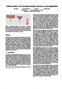
ABSTRACT We derive a conformal algebra treatment unifying all types of collisions among points, vectors, areas (defined by bivectors and trivectors) and 3D solid objects (defined by trivectors and quadvectors), based in a reformulation of collision queries from 3 to conformal 4,1 space. The algebraic formulation in this 5D space is then implemented in GPU to allow faster parallel computation queries. Results show expected orders of magnitude improvements computing collisions among known mesh models, allowing interactive rates without using optimizations and bounding volume hierarchies.

R

R

Categories and Subject Descriptors (according to ACM CCS): I.3.1 [Computer Graphics]: Hardware Architecture—Graphics processors, parallel processing, I.3.5 [Computer Graphics]: Computational Geometry and Object Modeling—Boundary representations, Collision detection, I.1.2 [Computer Graphics]: Algorithms—Algebraic algorithms

1. Introduction

C

E rtain

application domains, such as animation and haptic rendering, involve real-time interactions among detailed models, requiring fast computation of massive numbers of collisions. Diverse formulations and optimizations have been developed that individually target specific object representations for collision queries.

API/SDK [SK10] provides a SIMD parallel programming framework, with concurrent threads/simultaneous kernel execution at the GPU streaming processors. A current survey of GPU-assisted applications, including collision detection, can be found at [LMM10].

2.2. Geometric Algebra

In the next sections we present a unified geometric algebra treatment with a SIMD implementation that shifts collision detection from euclidean 3 to conformal 4,1 space. Line segments, spheres and polygons (and therefore, meshes) are treated as similar conformal entities by a shared core of CUDA kernels running in the GPU.

A recent formalism in Computer Graphics is the Geometric Algebra approach described by Dorst et al [DFM07], with the extensions to conformal geometric spaces added by Vince [Vin08]. The fundamental algebraic operators in this approach are the inner product (x · y), the outer product (x ∧ y), and the geometric product (xy).

Results show expected orders of magnitude improvements when computing collisions and intrusions among known mesh models, without using any hierarchical collision pre-filtering schemes.

Definition 2.1 For vectors a and b, the outer product a ∧ b defines an oriented hyperplane, or bivector. Its magnitude is the signed area of the parallelogram ka ∧ bk = kakkbk sin θ. The sign will be positive if a folds onto b counterclockwise, and negative otherwise.

2. Collision Detection Computation

Definition 2.2 For vectors a and b, its geometric product ab is the sum of the inner dot product and the outer bivector product.   anticommutative, ba = −ab ab = a · b + a ∧ b, associative, a(bc) = (ab)c = abc   distributive, a(b + c)d = abd + acd

R

B

R

A sically,

a collision is the result of a spatial query asking whether two geometric objects intersect at some point in time. A likely scenario is rigid body collision detection, highly used in haptic manipulation [ORC07, TFN10] and animation. Most techniques avoid exhaustive detection by enclosing objects into hierarchies of fast-to-discard bounding volumes [Eri05]: AxisAligned and Oriented Bounding Boxes (AABB, OBB), Rectangular Swept Spheres (RSS), Convex Hulls, kd-trees, and BSP trees.

2.1. GPU-assisted parallel computation General-Purpose Computation on Graphics Hardware [OLG∗ 07] harnesses programmable graphics processors to solve vastly complex problems, sending data as texture memory to shader programs for some number crunching instead of image rendering. On top of that, the Compute Unified Device Architecture (CUDATM )

† Co-financed in part by Project TIN2010-20590-C02-01 of the Spanish Ministry of Science (MEC) V Ibero-American Symposium in Computers Graphics – SIACG 2011

2.3. Conformal Geometry

Conformal Geometry [DFM07, DL09, BCS10] describes an elegant algebraic space for geometric visualization in 3 , since it is homogeneous, supports points and lines at infinity, preserves angle and distance, and can represent points, circles, lines, spheres and planes.

R

R

Definition 2.3 A conformal space p+1,q+1 of p + 1 positive dimensions and q + 1 negative dimensions is built from a p,q space. A point x = ue1 + ve2 + we3 in 3 maps to a null vector X in 4,1 (X · X = 0, X 6= 0), having the orthonormal base {e1 , e2 , e3 , e, e}. ¯

R

e1 · e1 = e2 · e2 = e3 · e3 = 1, n = e + e, ¯

n¯ = e − e¯

e · e = 1,

R

R

e¯ · e¯ = −1

X = P(x) = 2x + x2 n − n¯

(2.1)

E. Roa, V. Theoktisto, M. Fairén and I. Navazo / GPU Collision Detection in Conformal Geometric Space

154

Table 1: The 32 (1+5+10+10+5+1) blade terms of the canonical base for the conformal

1 5 10 10

Base Elements scalar vectors bivectors trivectors

5 1

quadvectors pseudoscalar (I)

Blade components e1 , e1 ∧ e2 , e2 ∧ e3 , e1 ∧ e2 ∧ e3 , e2 ∧ e3 ∧ e, ¯ e1 ∧ e2 ∧ e3 ∧ e, ¯

Blade type trivector trivector quadvector quadvector

Definition 2.4 The outer product of k vectors is called a k-blade:

R

k ≤ n+m

(2.2)

The highest order k-blade of a n,m space is called a pseudoscalar, denoted by I (I 2 = −1), for its similarity as a rotor to the complex number i. Thus, I X is a π2 counterclockwise rotation of X. Likewise, X I is a π2 clockwise rotation of X.

2.4. Intersections in conformal space n+m
= 2n+m A multivector is a linear combination of the ∑n+m k=1 k canonical base of blades for the conformal n,m space. Table 1 shows the 32 blade terms of the canonical base in 4,1 .

R

The meet operator (∨) denotes the intersection multivector, having pseudoscalar I = e1 e2 e3 ee¯ for that space. Intersections among multivector in the conformal model [DL09] are specified by the same equation for all multivectors, as shown in Table 3. B = (X ∨Y ) = (I X) ·Y, with square norm B2 = kBk2

(2.3)

¯ and B = β0 + βe1 e1 + . . . + βe1 e2 e1 e2 + . . . + βe1 e2 e3 ee¯ e1 e2 e3 ee. The work of Roa [Roa11] states the following criteria for B2 : If B2 > 0, X and Y intersect at least at two points. If B2 = 0, X and Y intersect at one point (a tangent). If B2 < 0, X and Y do not intersect. Table 3: Primitive intersections in Primitive Line Line Plane Plane Sphere

Primitive Plane Sphere Plane Sphere Sphere

R4,1 conformal space

Conformal representation B = Π1 ∨ L1 = (I Π1 ) · L1 B = S1 ∨ L1 = (I S1 ) · L1 B = Π1 ∨ Π2 = (I Π1 ) · Π2 B = S1 ∨ Π1 = (I S1 ) · Π1 B = S1 ∨ S2 = (I S1 ) · S2

3. Kernels for the Intersection Algorithms

F

e¯ e3 ∧ e, e¯ ∧ e e3 ∧ e1 ∧ e, e3 ∧ e¯ ∧ e e2 ∧ e3 ∧ e¯ ∧ e

3.1. Line Segment (Ray)–Triangle (Plane) intersection The intersection between a line segment and a triangle is a collision query between the ray passing along the segment and the plane of the triangle, and later checking whether boundaries meet. The intersection multivector B = (Π1 ∨ L1 ) = (I Π1 ) · L1 evaluates to B = (ω2 β3 + ω1 β4 − ω4 β1 )e1 e + (ω2 β3 + ω1 β4 − ω4 β1 )e1 e¯

+ (ω3 β1 − ω2 β2 + ω1 β5 )e2 e + (ω3 β1 − ω2 β2 − ω1 β5 )e2 e¯ + (−ω3 β3 + ω4 β2 + ω1 β6 )e3 e + (−ω3 β3 + ω4 β2 + ω1 β6 )e3 e¯

B

R

e, e1 ∧ e, e2 ∧ e, e3 ∧ e1 ∧ e, ¯ e2 ∧ e¯ ∧ e, e3 ∧ e1 ∧ e¯ ∧ e,

Geometric interpretation Three noncollinear points delimit the perimeter of the circle Two nonidentical points define a segment plus the point at infinity Four noncoplanar points delimit the surface of the sphere Three noncollinear points define a triangle plus the point at infinity

with n and n¯ representing the null vectors at infinity and at the origin. From these null vectors are derived the primitives shown on Table 2.

Rn,m ,

e2 ∧ e, ¯ e3 ∧ e, ¯ e1 ∧ e2 ∧ e, e1 ∧ e¯ ∧ e, e1 ∧ e2 ∧ e¯ ∧ e, e1 ∧ e2 ∧ e3 ∧ e¯ ∧ e

R4,1 conformal space, which also includes scalars, points and vectors

Algebraic representation C = P1 ∧ P2 ∧ P3 L = P1 ∧ P2 ∧ n S = P1 ∧ P2 ∧ P3 ∧ P4 Π = P1 ∧ P2 ∧ P3 ∧ n

v1 ∧ v2 ∧ . . . ∧ vk−1 ∧ vk = V ∈

λ e3 ,

e2 , e3 ∧ e1 , e1 ∧ e, ¯ e1 ∧ e2 ∧ e, ¯ e2 ∧ e3 ∧ e, e1 ∧ e2 ∧ e3 ∧ e,

Table 2: Algebraic primitives built from blades in the Primitive Circle Line Sphere Plane

R4,1 space

the next sections we present the algorithms, results and conclusions of the CUDA implementation for collision detection, using meshes from the Stanford University repository at http://www. graphics.stanford.edu/data/3Dscanrep/. Neither bounding volume hierarchies nor optimizations were employed, just raw collisions.

2

+ (−ω3 β4 − ω4 β5 − ω2 β6 )ee¯

(3.1)

= (ω3 β4 + ω4 β5 + ω2 β6 )

(3.2)

2

where the βs and the ωs are the coefficients of the corresponding multivectors for L1 and Π1 . A nonnegative B2 signals a potential collision. The segment is then tested against the triangle’s edges, to detect crossings and an effective collision. Algorithm 1 describes the complete procedure to compute intersections. Algorithm 1: Line Segment-Triangle intersection 1 k e r n e l S e g m e n t _ T r i a n g l e _ I n t e r s e c t ( s e g m e n t L1 , p l a n e P1 ) 2 N o r m a l i z e ( L1 ) ; N o r m a l i z e ( P1 ) 3 [ a , e 3 e r ] = C o n f o r m a l I n t e r s e c t L i n e P l a n e ( L1 , P1 ) 4 L3 = L i n e ( L0 . p o i n t 1 , L0 . p o i n t 2 ) 5 L2 = L i n e ( P1 . p o i n t 3 , P1 . p o i n t 1 ) 6 [ o u t 1 , i n d 1 ] = C o n f o r m a l I n t e r s e c t S e g m e n t S e g m e n t ( L2 , L3 ) 7 L2 = L i n e ( P1 . p o i n t 1 , P1 . p o i n t 2 ) 8 [ o u t 2 , i n d 2 ] = C o n f o r m a l I n t e r s e c t S e g m e n t S e g m e n t ( L2 , L3 ) 9 L2 = L i n e ( P1 . p o i n t 3 , P1 . p o i n t 2 ) 10 [ o u t 3 , i n d 3 ] = C o n f o r m a l I n t e r s e c t S e g m e n t S e g m e n t ( L2 , L3 ) 11 / / o u t # = 1 ( s e g m e n t s i n t e r s e c t ) ; 0 ( t h e y do n o t ) 12 / / ind #: s c a l a r c o e f f i c i e n t of e vector 13 i f ( a == 0 ) t h e n / / l i n e and p l a n e p a r a l l e l 14 i f e 3 e r = 0 t h e n / / l i n e l i e s on t h e t r i a n g l e ’ s p l a n e 15 / / v e r i f y segment i n t e r s e c t i o n with o t h e r t r i a n g l e s 16 r e t u r n ( o u t 1 ==1) or ( o u t 2 ==1) or ( o u t 3 ==1) 17 e l s e return 0 / / No i n t e r s e c t i o n f o u n d 18 end i f 19 e l s e / / w h e t h e r b o t h p o i n t s a r e i n same s i d e o f p l a n e 20 s i g n 1 = t r i v e c t o r ( P1 . p o i n t 2−P1 . p o i n t 1 , P1 . p o i n t 3−P1 . p o i n t 1 , L1 . p o i n t 1−P1 . p o i n t 1 ) 21 s i g n 2 = t r i v e c t o r ( P1 . p o i n t 2−P1 . p o i n t 1 , P1 . p o i n t 3−P1 . p o i n t 1 , L1 . p o i n t 2−P1 . p o i n t 1 ) 22 i f ( s i g n 1 == s i g n 2 ) t h e n 23 return 0 / / Segment d o e s n o t t o u c h p l a n e 24 end i f / / Segment c r o s s e s t h e p l a n e 25 r e t u r n r e s u l t = ( i n d 1 >0 and i n d 2 >0 and i n d 3 < 0 ) or 26 ( i n d 1