Granular Flows in Split-Bottom Geometries

Granular Flows in Split-Bottom Geometries Joshua A. Dijksman and Martin van Hecke Kamerlingh Onnes Lab, Universiteit Leiden, Postbus 9504, 2300 RA Leiden, The Netherlands (Dated: March 30, 2010) There is a simple and general experimental protocol to generate slow granular flows that exhibit wide shear zones, qualitatively different from the narrow shear bands that are usually observed in granular materials . The essence is to drive the granular medium not from the sidewalls, but to split the bottom of the container that supports the grains in two parts and slide these parts past each other. Here we review the main features of granular flows in such split-bottom geometries.

arXiv:1003.5620v1 [cond-mat.soft] 29 Mar 2010

PACS numbers: 45.70.Mg, 47.57.Gc, 83.50.Ax,

Granular media exhibit a complex mixture of solid and fluid-like behavior, often hard to predict or capture in models. Perhaps the most striking feature of granular flows is their tendency to localize in narrow shear bands [1]. A decent model of grain flows should be able to capture, and preferably, predict this type of behavior, but at present there is no general approach which, for given geometry, driving strength and grain properties, predicts the ensuing flow fields. In recent years, much progress has been made for fast flows, such as avalanche flows down an incline, where large flowing zones form. Microscopically, momentum exchange then takes place by a mixture of collisions and enduring contacts. This allows the definition of a dimensionless parameter I, the inertial number, which characterizes the local ”rapidity” of the flow. A local relation between stresses, strain-rates and I then successfully captures many aspects of these rapid granular flows [2–4]. In contrast, the situation for slow flows, such as those made by slowly shearing the boundaries of a container containing grains, is still wide open. The averaged stresses and flow profiles become essentially independent of the flow rate, so that constitutive relations based on relating stresses and strain rates are unlikely to capture the full physics. In this regime, shear banding is generally very strong, with shear bands having a typical thickness of five to ten grain diameters. These shear bands often localize near the moving boundary. For a recent review, see [1]. Experimental handles for probing this shear localization appears to be limited, since shear banding appears so robust. For example, granular flows in Couette cells always show the formation of a narrow shear band near the inner cylinder, irrespective of dimensionality, driving rate, or details of the geometry [5]. In this regime of slow flows, the inertial number I tends to zero and momentum transfer is dominated by enduring contacts. Soil mechanics is then a natural starting point to describe these flows, and both rate independence and shear banding are consistent with a Mohr-Coulomb picture where the friction laws acting at the grain scale are translated to the stresses acting at coarse-grained level. The idea is that when the ratio of shear to normal stresses is below the yielding threshold, grains remain quiescent, while in slowly flowing regions the shear stresses will be given by a (lower) dynamical yield stress. This way of

thinking readily captures the maximal slope of dry sand piles. However, the steep gradients associated with narrow shear bands are difficult to capture by a continuum theory, and shear bands often are described as having zero width [6]. Shearbands, then, are not always narrow. In this paper we will review recent experiments, numerical work and theoretical descriptions of wide shear zones which have been generated in so-called split-bottom geometries. The essence is to drive the granular medium not from the sidewalls, but to split the bottom of the container that supports the grains in two parts that slide past each other. By taking advantage of gravity to drive the granulate from the sliding discontinuity in the bottom support of the grain layer, one effectively pins a wide shear zone away from the sidewalls. The resulting grain flows are smooth and robust, with both velocity profiles and the location of the shear zones exhibiting simple, grain independent properties. The outline of this paper is as follows. In section I we will review the results of recent experiments and numerical work on the flows which have been generated in these special flow geometries. In section II we will discuss the theoretical ideas proposed to capture the flows observed in these geometries.

I.

SLOW FLOWS IN THE SPLIT-BOTTOM GEOMETRY: PHENOMENOLOGY A.

General Description

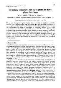
In this section, we focus on the rate independent regime which is reached for slow enough driving. Two variants of the split-bottom geometry will be encountered: in experiments one typically employs a cylindrical split-bottom shear cell, consisting of a bucket, at the bottom of which a disc rotates with respect to the bucket (Fig. 1a) [7–10], while for theoretical studies the linear split-bottom cell with periodic boundary conditions is more convenient (Fig. 1b) [11–14].

2

FIG. 1: (a) Cylindrical split-bottom geometry, showing a disc of radius Rs at the bottom of a granular layer of depth H. Here, the outer cylinder rotates with rate Ω and the bottom disc is kept fixed – A similar geometry, with fixed outer cylinder and rotating disc is also frequently encountered. (b) Linear split-bottom geometry, where a container is split along a straight line in its bottom. This geometry can be seen as the Rs → ∞ limit of the cylindrical cell. (c) The transition in flow structure from shallow to deep flows in the cylindrical split-bottom geometry. In the dark grey region the material essentially co-moves with the disk.

B.

Parameters and Regimes

The cylindrical split-bottom geometry is characterized by three parameters. The radius of the bottom disc Rs and its rotation rate Ω are generally fixed in a set of experiments, and the relative motion of disc with respect to the cylindrical container drives the flow. The thickness of the granular layer, H, is the control parameter that typically is scanned in a series of experiments. Note that the radius of the container appears immaterial, as long as it is sufficiently large; 25% larger than Rs appears to be sufficient [8]. We denote the ratio of the averaged azimuthal velocity of the grains vθ (r)/r and the disk rotation speed Ω by ω; ω = 0 thus corresponding to stationary grains, while ω = 1 corresponds to grains co-moving with the driving. For the small Ω of interest here (typically less than 0.1 s−1 ), the flow profiles ω(r, z) are independent of Ω – the flow is rate independent, and transients are short lived. Since centrifugal forces are negligible for typical sizes of Rs (typically a few cm), one may also fix the disc and rotate the bucket, and essentially obtain the same sort of flows with ω ˜ (r, z) = 1 − ω(r, z) – see [7–9]. The two parameters H and Rs set the large-scale structure of the flow. When the disk rotates, a shear zone propagates from the slip position Rs upwards and inwards. The qualitative flow behavior is governed by the ratio H/Rs , and three regimes can be distinguished – Fig. 1c. A regime of shallow layers is found for H/Rs < 0.45, and

FIG. 2: (a) Surface flows for glass beads of diameter 300 µm and a range of filling heights H as indicated are well described by an error function (fit not shown) - Rs = 85 mm here, and the outer cylinder is rotating. (b) Collapse of the surface flow profiles shown in (a) and comparison to error function. The rescaled radial coordinate λ is defined as (r − Rc )/W . Top inset: strain rates are Gaussian. Bottom inset: the tail of flow profile corresponds well to the Gaussian tail of the error function. Figure adapted from Ref. [7].

here the shear zone reaches the free surface. The threedimensional shape of the shear zones is roughly that of the cone of a trumpet, with the front of the trumpet buried upside down in the sand. Another regime of deep layers plays a role for H/Rs > 0.65, and here the shear zone essentially forms a dome-like structure in the bulk of the material; little or no shear is observed at the free surface. In between there is an intermediate regime, where the shear in the bulk of the material is a mix between the trumpet and dome-like shape. C.

Surface Flow

Shallow layers — We first focus on the flow observed at the free surface. For shallow layers, a narrow shear zone develops above the split at Rs , and when H is increased, the shear zone observed at the surface broadens continuously and without any apparent bound. Additionally, with increasing H, the shear zone shifts away from Rs towards the center of the shear cell (Fig. 2a). After proper rescaling, all bulk profiles collapse on a universal curve which is extremely well fitted by an error function:

ω(r) =

1 1 r − Rc + erf { }, 2 2 W

(1)

where erf denotes the error function, r is the radial coordinate, Rc the center of the shearband (where ω(r) = 0.5) and W the width of the shearband (Fig. 2). Accurate measurement of the tail of the velocity profile further validate Eq. (1), and rule out an exponential tail of the velocity profile (Fig. 2b). The strain rate is therefore Gaussian, and the shear zones are completely determined by their centers Rc and widths W . Particle shape does not influence the functional form of the velocity profiles [8], in contrast to the particle dependence found for wall-localized shear bands in a Couette

3

FIG. 3: (a) Shear zone positions Rc versus H, where Rs = 95, 85, 75, 65, and 45 mm. Lines correspond to Eq. 2. (b) Log-log plots of W for spherical glass beads of increasing sizes (ranging from average diameter 300 µm to 2 mm) for Rs = 95 mm. The lines shown in (b) correspond to exponents of 1/2, 2/3, 1. Figure adapted from [8].

cell [5]. For these, the vicinity of the wall induces particle layering, in particular for monodisperse mixtures. Apparently such layering effects play no role for these bulk shear zones, where it should be noted that the effects of shear-induced ordering of particles with larger aspect ratios has not yet been investigated. Remarkably, the center of the shear zone, Rc , turns out to be independent of the material used (Fig. 3a). Therefore, the only relevant length-scales for Rc appear to be H and Rs . We find that the dimensionless ’displacement’ of the shear zone, (Rs − Rc )/Rs , is a function of the dimensionless height (H/Rs ) only. The simple relation (Rs − Rc )/Rs = (H/Rs )5/2

(2)

fits the data well (Fig. 3a). The relevant length scale for the shear zone width W defined above is given by the grain properties, and is independent of Rs (Fig. 3b). Grains shape, size, and type also influence W (H): irregular particles display smaller shear zones than spherical ones of similar diameter. The best available experimental data shows that W/d ∼ (H/d)2/3 ,

(3)

where d denotes the particle diameter. Although this scaling has not been checked over more than a decade, the exponent is clearly not equal to 1/2 or one. As yet there is no explanation for this scaling. The available numerical data coming from molecular dynamics simulations essentially confirm this picture [10, 12, 13, 15]: the surface flows in split-bottom geometries for H/Rs < 0.45 are given by Eqs. 1-3. Only the absolute width of the shear zone at the surface W (z = H) remains as a fit parameter, but once this width has been measured for a single value of H/Rs , Eq. 3 can be used to estimate the width for the whole range of H/Rs < 0.45.

FIG. 4: Core precession in a split-bottomed geometry. (a-d) Series of snapshots of top views of a setup with stationary disc and rotating outer cylinder (for Rs = 95 mm, H = 60 mm, and rotation rate Ω = 0.024 rps), where colored particles sprinkled on the surface illustrate the core precession for t = 0 s (a), t = 10 s (b), t = 100 s (c) and t = 1000 s (d). (e) Data collapse of the precession rate ωp for Rs = 45 mm (diamonds), Rs = 65 mm (x) and Rs = 95 mm (circles) when plotted as a function of H/Rs . Figure adapted from Ref. [9].

Deep Layers — When H/Rs is small, the core material rests on and co-moves with the center disc. With increasing H/Rs , the width of the shear zone grows continuously, and its location moves inward towards the central region (Eq. 2). This implies that for deep layers qualitatively different flow patterns can be expected to occur. The most striking feature of these flows is that the core, as observed at the free surface, precesses with respect to the bottom disc for H/Rs & 0.65 — hence material in the central part of the system no longer rests on the disc, and there is torsional failure of the core. Precession is not simply a consequence of the overlap of two opposing shear zones, since before being eroded by shear, the inner core rotates as a solid blob for an appreciable time (Fig. 4a-d). The precession rate ωp is defined as the limit of ω(r) for r going to zero, where we assume, for simplicity, that the outer bucket rotates with rate Ω and the bottom disc is kept fixed, as in [9] – consistent results are found in a setup where the disc was rotated and the outer cylinder kept fixed [10]. For various slip radii, the onset height for precession grows with Rs , and the data for ωp collapses when plotted as a function of H/Rs, see Fig. 4e). When H/Rs becomes of order one, the whole surface rotates rigidly with the rotating drum and all shear takes place in the bulk of the material; on the other hand, for H/Rs < 0.65, hardly any precession can be observed. Intermediate regime — In the intermediate regime, 0.45 < H/Rs < 0.65, a precursor to the transition to precession can be observed, since a careful analysis reveals that the surface velocity profiles ω(r) increasingly become asymmetric for H/rs > 0.45. In fact, one can

4

FIG. 6: Contours of constant angular velocity ω, for different filling height H. Upper panels: MRI experiments: ω = 0.84 (diamonds), 0.24 (squares), 2.4 × 10−2 (circles), 2.4 × 10−3 (triangles), and 2.4 ×10−4 (inversed triangles). Dashed lines indicate H and dotted lines are guides to the eye. Lower panels: simulations. Color is used to identify velocity ranges: dark red, ω ∈ [0.84, 1]; orange, ω ∈ [0.24, 0.84]; yellow, ω ∈ [2.4 × 10−2 , 0.24]; green, ω ∈ [2.4 × 10−3 , 2.4 × 10−2 ]; blue, ω ∈ [2.4 × 10−4 , 2.4 × 10−3 ]; grey, ω ∈ [0, 2.4 × 10−4 ]. Figure reprinted with permission from [10]. Copyright (2006) American Physical Society. FIG. 5: Surface velocity profiles ω(r) for Rs = 95 mm and increasing layer depth H. Thick curves: H = 10, 20 . . . 80 mm; Thin curves H = 15, 25, . . . 75 mm; Dashed curves H = 56, 57, . . . 69 mm. (a) Precession gradually sets in for H > 60 mm. (b) Corresponding profiles of χ(r) (dots, see Eq. 4), compared to cubic fits given by Eq. 5 (curves). Figure adapted from [9].

Rc at the free surface. Then to obtain Rc at depth z, one imagines a systems with a depth of H − z, and by inverting Eq. 2, obtains where the split would have to be in a system of depth of H − z for the surface location to be as given [6]. Identifying the split at depth H − z with the center of the shearband Rs (H − z), this yields:

generalize Eq. 1 by writing 1 1 ω(r) = + erf (χ(r)) , 2 2

(4)

and by fitting the data for ω(r) over the whole range of H/Rs to this equation (Fig. 5), one finds that χ(r) can be fitted well by a cubic polynomial of the form χ(r) = a0 + a1 r + a3 r3 .

(5)

For shallow layers, a3 = 0, and a0 and a1 follow from the scaling laws Eqs. 2 and 3. For 0.45 < H/Rs < 0.65, a3 starts to grow and governs the symmetry breaking of the flow profiles, while for deep layers (H/Rs > 0.65), a1 tends to zero, and a two parameter fit describes the flow profiles well again [9].

D.

Bulk Flow

Shallow flows – The bulk structure of granular flows is harder to access, but by now, we have information on split-bottom flows from experiments that bury and excavate colored beads [8], Magnetic Resonance Imaging (MRI) [10, 16] and numerical simulations [10, 12, 13, 15] (see Fig. 6). First, for shallow layers, the flow profiles at fixed depth z below the surface H still takes an error function form, which allows us to characterize ω(r) at fixed z with the same two parameters Rc and W as before. The location of the shear zones in the bulk where found to be consistent with a scaling argument put forward by Unger et al.. The idea is follows: Eq. 2 gives the location

 1/2.5 z = H − Rc 1 − Rc /Rs (1 − H/Rs )2.5 ) .

(6)

The width W (z) of the shear zones is harder to obtain reliably, but the best available experimental data suggest a power law growth of the form W ∼ z α , where α is less than 1/2 and more than 1/4 [8, 11]. More recent numerical studies [13] found that W (z) can also be well described by a “quarter circle” curve of the form p (7) W (z) = W (z = H) 1 − (1 − z/H)2 . Deep Layers – The symmetry breaking and the eventual disappearance of grain motion at the surface indicates that qualitatively different bulk flow is developing: the trumpet shape of the shear zones present in shallow layers must have changed. When H/Rs is sufficiently large, the shear zone is entirely confined to the bulk of the material, and forms a dome-like structure above the rotating disk [6, 9, 10, 16] – see Fig. 6. The torsional failure of the material is thus concentrated in the dome. Cheng et. al. measured the functional form of the axial velocity profile ω(z)|r=0 , and found it to be described by a Gaussian: ω(z, r = 0) = ωp + (1 − ωp ) exp −z 2 /(2σ 2 ) ,

(8)

where ωp is the rotation rate observed at the surface at r = 0, which decreases roughly exponentially with H, and σ, the width of the bulk Gaussian velocity profile, is approximately Rs /5 [10]. More recent experiments find a slightly different functional dependence on z [17]. Couette versus split-bottom geometries –

5

FIG. 7: Surface flow profiles observed for 1 mm glass beads in a split-bottom Couette geometry, with inner cylinder radius Ri = 40 mm, a split at Rs = 65 mm, and H = 10, 30, 40, 50, 60, 70, 80, 100, 110 mm. The outer cylinder is 120 mm. Figure from Ref. [18].

The first studies [7] of split-bottom geometries where done in a modified Couette cell, as shown in Fig. 7. The resulting flows are similar to the disc geometry, as long as the shear flow is away from the side walls, but since for increasing filling heights the shear zones move inward, they will inevitably ’collide’ with the inner cylinder for sufficiently large filling height. The resulting flow profiles are shown in Fig. 7 [18]. First, one observes that for sufficiently large H, the flow profiles become independent of H. The main result is that the tail of these flow profiles becomes purely exponential for large H, while it is Gaussian for shallow H. We have found this exponential tail to be robust, i.e., independent of grain shape. Note that this does not contradict the findings of Mueth et al. – these concern the shape of the flow profile near the shearing wall, corresponding to the range 10−3 < ω < 1 – flow profiles are indeed grain dependent here. But further out in the tail they become purely exponential. For other examples of exponential tails see [19].

FIG. 8: Evolution of dilatancy. (a) Color map of relative density change (light blue corresponds to -10%) for H/Rs = 0.51 after 4 rotations of the bottom disk (b) Spread of dilated zone for vertical shear observed in the bulk at H/Rs = 0.51 at z = 22 mm (H = 36 mm), for N = 1/2, 1, 2, . . . , 64, compared to estimates where, after N turns, the local strain equals one. (c) Spread of dilatancy for dome-like flow observed at H/Rs = 0.77, for number of disc rotations N as indicated. Figure adapted from Ref. [16].

the strain rate [20]. Consistent with this, the dilated zone was found to slowly spread throughout the system as time progresses (Fig. 8). This spread is consistent with the idea that, after initial preparation, the accumulated local strain governs the amount of dilatancy. To show this, the flow field in the bulk was reconstructed by combining the above mentioned scaling relations for the location and width of the shear zones in the bulk, and this reconstructed flow field can then be compared to the density field obtained by MRI. Such comparison shows that the locations of the dilated zone and the shear zone coincide, for small filling heights (H/Rs < 0.6). Finally, for deep filling heights where torsional failure and precession play a role, a relatively long-lived transient was found to cause the dilated zone to deviate substantially from the late-time shear zone.

II. E.

Dilatancy

By means of MRI, direct measurements of the evolution of the local packing density of the shear flow generated in a cylindrical split-bottomed geometry were performed in [16]. To be able to image the particles by means of MRI, food grade poppy seeds were used; these contain MRI-detectable mineral oils. It was observed that the relative change in density in the flowing zone is rather strong and saturates around 1015 % – likely the rough and peanut shape of the poppy seeds plays a role. After long times, a large zone with essentially constant low packing fraction forms, encompassing most of the shearband. The fact that the density remains constant here, even though local strain rates vary over many decades, suggests that the density of the flowing material is a function of the total strain, and not of

FLOWS IN THE SPLIT-BOTTOM GEOMETRY: THEORY

The flows in split-bottom geometries have been simulated both by molecular dynamics simulations [10, 12, 15] as well as by contact dynamics [13], and a number of theoretical approaches have been put forward. It remains remarkable that no single consistent theoretical framework is available from which Eqs. 1-3 can be deduced. Creating such a theory would constitute an important milestone in the development of our understanding of slow granular flows. Here we discuss the main approaches to flows in the split-bottom geometry. Variational principle – The first attempt to describe the flows in split-bottomed geometries goes back to Unger and coworkers [6]. The flows are treated in a Mohr-Coulomb fashion, with shear bands of zero width.

6 The idea is to minimize the energy dissipation needed to sustain the flow. Calculating the total friction along the shear-sheet r(z) using assumptions of constant friction coefficient µ and hydrostatic pressure P , amounts to finding the minimum of the functional (see Fig. 9) Z T (H) = 2gπρφµ

H

(H − z)r2

p

1 + (dr/dz)2 dz

(9)

0

Here ρ is the bulk density of the particles, φ is the average packing fraction (∼ 0.59 [4]) and µ is the effective friction coefficient. Identifying r(z) with the center of the shearband Rc (z), minimizing Eq. 9 gives predictions for the location of the shearbands in the split-bottom geometry. The location of the shear zones predicted for shallow layers are very close to those observed, and for deep layers the model predicts a hysteretic transition to dome-like shear. Hence, while a number of aspects of split-bottom flows can be captured by this simple model, the hysteretic transition and zero width of the shear bands are clearly in contrast to experimental findings.

FIG. 9: (a) An arbitrary shear zone of zero width r(z) separates a rotating inner core and a static outer body. In (b): The frictional stress σrθ = µP on the shearing surface can be integrated to give the total driving torque necessary to rotate the disk in red. The integral is given in Eq. 9.

Extending the variational principle – To explain the broad shearbands in the split-bottom geometry, a random or randomly varying local material failure strength [14, 21] was invoked. The main extension extends the minimal dissipation model by combining the variational principle with a self organized random potential as follows. At any given time, the shear band is represented as having zero width. However, the granular material is now taken to be inhomogeneous, with a local strength field which varies with space and is updated every timestep. At any given time the surface that minimizes the torque can be obtained, after which the strength field is updated etc. A smooth flow profile is then obtained by averaging over the different shear bands. The resulting flow fields are very close to those observed experimentally, with the only adjustable parameter controlling the effect of disorder. One possible point of criticism is that the model assumes that the fluctuating shear bands are radially symmetric – see [14] for details. The main findings of [21] where confirmed by a different but related approach by Jagla [14], and recently a two dimensional model using stochastic interparticle forces was shown to be able to also generate shear bands of finite width [22].

FIG. 10: (a) Shear free sheets in a linear shear geometry. (b) Stress components acting in material (c) Shear free sheets in curved geometry. (d) Stress ratios in section of linear geometry, showing that the stresses are of the form of Eq. 10, and that the friction coefficient µ = −σ23 /σ33 is not completely constant. Figure adapted from Ref. [12].

Inertial flows – Jop performed simulations of flows in a cylindrical split-bottom setup [23], using the inertial number theory, which should be valid for faster flows [4]. The location of the shear zones in the bulk, the smooth transition to precession and the dome flows were all recovered. The width of the shear zones was found to scale with driving rate as Ω0.38 , and indeed for slow flows the shear zones attain zero width. The inertial model therefore does not fully capture the physics of the slow split-bottom flows, but

Shear free sheets – The form of the stress tensor in slow granular flows is a matter of debate. From a soil mechanics perspective, there is no reason to assume that the principle directions of stress and strain rate align, but Depken and coworkers have suggested that once there is flow in the system, the principle directions do align. The idea is that flow, even at a distance, creates sufficient amount of agitation that any amount of shear stress should lead to flow – in other words, once there is flow, there is no clear yielding threshold anymore [11, 12, 17].

it does slightly better than Ungers original model [6] in that it captures the smooth transition to precession. The only experimental work so far on rate dependent flows in the split-bottom is the work by Corwin [24]. He however described flows for which the centripetal forces dominate the gravitational and hydrostatic forces, which are outside the regime of flow rates studies by Jop.

7 Coaxiality severely restricts the form of the stress tensor, and for steady grain flows the flow can be decomposed into so-called shear free sheets (SFS), that slide past each other – there is no (average) grain motion within the sheets (Fig. 10a-c). In this SFS basis, the stress tensor takes the form:  P0 0 0 = 0 P τ  . 0 τ P

structure of this model is incapable of capturing the observed wide shearbands – the model’s only lengthscale is the spot size, and therefore cannot yield wide shearbands. Moreover, its use of Mohr-Coulomb plasticity theory is in conflict with the observed co-axiality [12, 13] of the stress and strain tensors.



σSFS

(10)

The form of the stress tensor is reminiscent of that of the inertial model [3], but with the exception that the stresses P and P 0 do not need to be equal (they are not in fact – see Fig. 10), and that the friction coefficient µ := τ /P does not depend on flow rate, since the flows are rate-independent. However, as Depken showed [11], µ cannot be constant if the shear zones have finite width, and in fact has to attain a local maximum within the shear zone – as subsequent numerical simulations indeed found [12, 13]. Recent contact dynamics simulations of Ries et al. in linear split-bottom cells [13] have confirmed that the stress and strain tensors align, so that the stresses take the form given by Eq. 10. The alignment also occurs in the absence of gravity (to carry out these simulations, a mirror of the system was added; see Fig. 7 in [13]). Perhaps surprisingly, gravity appears not to be important for the understanding of split-bottom flows.

III.

OUTLOOK

Spot model — To describe rate-independent flows in general, Bazant and coworkers put forward the ’spot’-model, which is based on the assumption that slow, dense granular flows are best described with a diffusion of low density regions in the material, called spots [25]. The two-dimensional model describes flow profiles in chute flow and Couette geometries reasonably well. However, recently it was shown [26] that the very

The surprising, robust and universal properties of slow granular flows in split-bottom geometries have made the split-bottom geometry into a versatile testing ground, not only for models of slow flows, but also for experimental studies of related flows, of mixtures and segregation [27], of non-local flows [17], of faster grain flows [24, 28] and of suspension flows [29]. So far, no single convincing continuum theory to describe the wide shear zones generated in split-bottom shear cells has been put forward — even though the experimental results strongly suggest that these flows should be amenable to a continuum description. The failure of the Mohr-Coulomb approach to describe the internal structure of narrow shear bands might not be troublesome, but its failure to describe these much wider shear zones is cause for concern. Apart from the theoretical challenges and experimental use of the split-bottom geometry, the broad shear zones occurring in this geometry allow for further experiments on slow flows, that are more difficult to realize in narrowly localized shear bands. Open questions for the future include to understand the microscopic organization and velocity fluctuations in these flows, to understand the role of interstitial fluid and grain shape, and to explore the range of much smaller, but in particular much faster driving rates.

[1] P. Schall and M. van Hecke, Ann. Rev. Fluid Mech., 2010, 42, 67–88. [2] G. MiDi, Eur. Phys. J. E, 2004, 14, 341–365. [3] Y. F. P. Jop and O. Pouliquen, Nature, 2006, 441, 727– 730. [4] Y. Forterre and O. Pouliquen, Ann. Rev. Fluid Mech., 2008, 40, 1–24. [5] D. M. Mueth, G. F. Debregeas, G. S. Karczmar, P. J. Eng, S. R. Nagel and H. M. Jaeger, Nature, 2000, 406, 385–389. [6] T. Unger, J. T¨ or¨ ok, J. Kert´esz and D. E. Wolf, Phys. Rev. Lett., 2004, 92, 214301. [7] D. Fenistein and M. van Hecke, Nature, 2003, 425, 356. [8] D. Fenistein, J.-W. van de Meent and M. van Hecke, Phys. Rev. Lett., 2004, 92, 094301. [9] D. Fenistein, J.-W. van de Meent and M. van Hecke, Phys. Rev. Lett., 2006, 96, 118001.

[10] X. Cheng, J. B. Lechman, A. Fernandez-Barbero, G. S. Grest, H. M. Jaeger, G. S. Karczmar, M. E. M¨ obius and S. R. Nagel, Phys. Rev. Lett., 2006, 96, 038001. [11] M. Depken, W. van Saarloos and M. van Hecke, Phys. Rev. E, 2006, 73, 031302. [12] M. Depken, J. B. Lechman, M. van Hecke, W. van Saarloos and G. S. Grest, EPL, 2007, 78, 58001 (5pp). [13] A. Ries, D. E. Wolf and T. Unger, Phys. Rev. E, 2007, 76, 051301. [14] E. A. Jagla, Phys. Rev. E, 2008, 78, 026105. [15] S. Luding, Particulate Sci. and Techn., 2008, 26, 33–42. [16] K. Sakaie, D. Fenistein, T. J. Carroll, M. van Hecke and P. Umbanhowar, EPL, 2008, 84, 49902. [17] K. Nichol, A. Zanin, R. Bastien, E. Wandersman and M. van Hecke, arXiv, 2009, 0911.4635. [18] R. Mikkelsen, Ph.D. thesis, University of Twente, 2005. [19] J. Crassous, J.-F. Metayer, P. Richard and C. Laroche,

8 J. Stat. Mech., 2008, P03009 (15pp). [20] A. J. Kabla and T. J. Senden, Phys. Rev. Lett., 2009, 102, 228301. [21] J. T¨ or¨ ok, T. Unger, J. Kert´esz and D. E. Wolf, Phys. Rev. E, 2007, 75, 011305. [22] A. Bordignon, L. Sigaud, G. Tavares, H. Lopes, T. Lewiner and W. Morgado, Phys. A, 2009, 388, 2099 – 2108. [23] P. Jop, Phys. Rev. E, 2008, 77, 032301. [24] E. I. Corwin, Phys. Rev. E, 2008, 77, 031308.

[25] W. W. Mullins, J. Appl. Phys., 1972, 43, 665–678. [26] E. Woldhuis, B. Tighe and W. van Saarloos, Eur. Phys. J. E, 2009, 28, 73 – 78. [27] K. M. Hill and Y. Fan, Phys. Rev. Lett., 2008, 101, 088001. [28] J. Dijksman, Ph.D. thesis, Leiden University, 2009. [29] J. Dijksman, S. Slotterback, E. Wandersman, C. Berardi, W. D. Updegraff, M. van Hecke and W. Losert, in preparation.