Graph-based Intrusion Detection on Massive Process Traces - arXiv

GID: Graph-based Intrusion Detection on Massive Process Traces for Enterprise Security Systems

arXiv:1608.02639v1 [cs.CR] 8 Aug 2016

Boxiang Dong∗ , Zhengzhang Chen† , Hui Wang∗ , Lu-An Tang† , Kai Zhang† , Ying Lin‡ , Wei Cheng† , Haifeng Chen† and Guofei Jiang† ∗ Stevens Institute of Technology, Hoboken NJ † NEC Laboratories America, Princeton NJ ‡ University of Washington, Seattle WA

Abstract—Intrusion detection system (IDS) is an important part of enterprise security system architecture. In particular, anomaly-based IDS has been widely applied to detect abnormal process behaviors that deviate from the majority. However, such abnormal behavior usually consists of a series of lowlevel heterogeneous events. The gap between the low-level events and the high-level abnormal behaviors makes it hard to infer which single events are related to the real abnormal activities, especially considering that there are massive “noisy” low-level events happening in between. Hence, the existing work that focus on detecting single entities/events can hardly achieve high detection accuracy. Different from previous work, we design and implement GID, an efficient graph-based intrusion detection technique that can identify abnormal event sequences from a massive heterogeneous process traces with high accuracy. GID first builds a compact graph structure to capture the interactions between different system entities. The suspiciousness or anomaly score of process paths is then measured by leveraging random walk technique to the constructed acyclic directed graph. To eliminate the score bias from the path length, the Box-Cox power transformation based approach is introduced to normalize the anomaly scores so that the scores of paths of different lengths have the same distribution. The efficiency of suspicious path discovery is further improved by the proposed optimization scheme. We fully implement our GID algorithm and deploy it into a real enterprise security system, and it greatly helps detect the advanced threats, and optimize the incident response. Executing GID on system monitoring datasets showing that GID is efficient (about 2 million records per minute) and accurate (higher than 80% in terms of detection rate). Keywords-Enterprise security system; intrusion detection; graph modeling; anomaly detection; random walk; path searching

I. I NTRODUCTION With computers and networked systems playing indispensable roles in almost every aspect of modern world of society such as industry, government, and economy, cyber-security undoubtedly bears the utmost importance in preserving right social orders. However, nowadays, serious cyber-attacks still keep happening, which causes significant financial loss and public tensions. One example is the leakage of sensitive, highprofile information from giant marketing establishments or financial institutions. According to a recent study by Ponemon Institute and IBM [4], data breaches cost companies an average of $201 per record in 2014, and the total cost paid by organizations reaches $5.9 millions.

To guarantee the information security in the network of computers, an intrusion detection system (IDS) is needed to keep track of the running status of the entire network and identify scenarios that are associated with potential attacks or malicious behaviours. Compared to signature-based methods, which can only detect attacks for which a signature has previously been created, anomaly-based intrusion detection aims at identifying unusual entities, events, or observations from a running system that deviate from its normal pattern of behaviours. Detected anomaly patterns can be translated into critical actionable information that can significantly facilitate human decision making and mitigate the damage of cyberattacks. Towards this end, anomaly-based intrusion detection, with a variety of algorithms proposed in recent years (e.g., [16], [14]), turns out to be a particularly useful tool. However, building an efficient and accurate anomaly-based intrusion detection system is still challenging due to the nature of the system monitoring data. However, building an efficient and accurate anomaly-based intrusion detection system is still challenging due to the nature of the system monitoring data. First, IDS typically deals with a large volume of system event data (normally more than 10, 000 events per host per second) to detect possible malicious activities. Second, the variety of system entity types may necessitate high-dimensional features in subsequent processing. Such enormous feature space could easily lead to the problem, coined by Bellman as “the curse of dimensionality” [2]. More importantly, IDS often relies on a coordinated or sequential, not independent, action of several system events to determine what state a given system is in. The system monitoring data are typically low-level interactions between various entities (e.g., a program opens a file or connects to a server) with exact time stamps, while abnormal behaviors such as attempted intrusions are higher-level activities which usually involve multiple different events. For example, a network attack called Advanced Persistent Threat (APT) is composed of a set of stealthy and continuous computer hacking processes, by first attempting to gain a foothold in the environment, then using the compromised systems as the access into the target network, followed by deploying additional tools that help fulfill the attack objective. The gap between the low-level events (e.g., process events) and the high-level abnormal behaviors (e.g., APT attacks) makes it

hard to infer which events are related to the real abnormal activities, especially considering that there are massive “noisy” low-level events happening in between. Hence, the approaches [23], [27] that identify individual events that confer a given system state are inappropriate to detect sequences of such interactions between different events. Therefore, there exists a vital need for the methods that can detect the sequences of events that are related to the abnormal activities in an efficient and accurate way. To address the aforementioned challenges, in this paper, we introduce GID, a graph-based intrusion detection algorithm to capture the interaction behavior among different entities, which sheds important light on event sequences (or sequence patterns) that are related to anomalous behavior. A key proposal to achieve this is a compact graph representation that preserves all useful information from the massive heterogeneous system monitoring data. Then, a random-walk based algorithm on this graph is conducted to provide anomaly scores that quantify the “rareness” or anomaly degree of the event sequences with regards to the historical data. Existing randomwalk based anomaly detection algorithms (e.g., [6], [7]) can only be applied to detect single suspicious entities/events. By introducing the sender and receiver scores, we extend the random-walk technique to detect suspicious process paths, and prove its convergence in the directed acyclic graph. To eliminate the potential score bias from the path length, we use the Box-Cox power transformation based approach to normalize the anomaly scores so that the scores of paths of different lengths have the same distribution. To improve the detection accuracy, we perform the validation of the suspicious event sequences to ensure that the abnormal event sequences are sufficiently deviated from normal ones. We further propose an optimization scheme by integrating the threshold algorithm with the detection algorithm to improve the efficiency. We launch an extensive set of experiments on a testbed that simulates the real-world attacks on the real enterprise system, to evaluate the time performance and detection accuracy of our approach. The results demonstrate that, on an enterprise surveillance data that contain 440 million system events, GID is efficient (as much as 2 million records per minute) and accurate (higher than 80% in terms of detection rate). We fully implement our GID system and deploy it into a real enterprise security system, which greatly helps detect advanced threats, and optimize the incident response. To summarize, in this paper we make the following contributions: • We identify an important problem (suspicious process path discovery) in intrusion detection, and design a compact graph model to preserve all the useful information from massive system monitoring data; • We develop a suspicious path discovery algorithm based on random walk and Box-Cox power transformation. By introducing the sender and receiver scores, we extend the random-walk technique to detect suspicious sequences in the directed acyclic graphs, and prove its convergence; • We propose a fast optimization technique to avoid check-

ing all candidate paths; We apply our algorithm to real enterprise surveillance data and demonstrate its effectiveness and efficiency. The rest of the paper is organized as follows. Section II formally states our problem. Section III discusses our graph-based intrusion detection approach in detail. Section IV presents the optimization scheme to improve the efficiency. Section V provides the experiment results. Section VI discusses the related work. Finally, Section VII concludes the paper. •

II. P RELIMINARIES In this section, we present the preliminaries of our work. For the following sections, we assume that the computer system is UNIX system, for simplicity of discussion. System Entities. System monitoring data, collected by our agent, indicates the interactions between a set of system entities. We consider four different types of system entities: (1) files, (2) processes, (3) Unix domain sockets (UDSockets), and (4) Internet sockets (INETSockets). Each type of entities is associated with a set of attributes. Two types of interactions between the system entities are considered in this paper: (1) file accessed by the processes; and (2) communication between processes. According to the design of modern operating systems, sockets function as the proxy for different processes to communicate. Typically, two processes that execute on the same host communicate with each other via UDSockets, while processes on different hosts communicate with each other by INETSockets. Thus, on a single host, the interactions exist between the following types of entities: (1) processes and files, (2) processes and processes, (3) processes and sockets (both UDSockets and INETSockets), and (4) UDSockets and UDSockets. System Events. We model the interactions between entities as system events. Formally, a system event e(nb , nd , t) is a record contains source entity nb , destination entity nd , a timestamp t when e happens. nb and nd are different entities from possibly different types. In computer systems, a heterogeneous event is a record involving entities of different types such as the files, processes, Unix domain sockets (UDSockets), and Internet sockets (INETSockets). And the following types of entity interactions are allowed in UNIX: (1) processes and files, (2) processes and processes, (3) processes and sockets (both UDSockets and INETSockets), and (4) UDSockets and UDSockets. System events can be generated at a high frequency (e.g., 20, 000 events per second). In a modern computer system, plentiful system events can happen without users’ awareness. For instance, the Exim process, which is the mail transfer agent, frequently accesses the /etc/hosts file to check the mapping between host names and IP addresses. Event Sequence. System events often happen in a chain. For instance, process A first opens file F , then reads F , and sends the content of F to process B. We formulate such chain as the event sequence. Formally, a sequence of events e1 , . . . , eℓ−1 that happens in a chain is denoted as S{e1 , e2 , . . . , eℓ−1 }, where ei .nd = ei+1 .nb , i.e., ei ’s destination entity is the ei+1 ’s

source entity, and ei .t < ei+1 .t for i ∈ {1, . . . , ℓ − 1}. The length of S is ℓ. The timespan of a event sequence is ts = eℓ−1 .t−e1.t. A simplified representation is to denote the event sequence as S{n1 , n2 , . . . , nℓ−1 , nℓ }, informing that the data is transmitted from n1 to nℓ , via n2 , . . . , nℓ−1 following the time order. Abnormal Event Sequence. Most of the abnormal system behaviors, such as cyber intrusion, spying, and information stealing, often exploit event sequences to achieve their goals. Typically these event sequences, not individual events, behave differently from the regular event sequences (see formal definition of abnormality in Section III-E). We call those event sequences that are associated with malicious behaviors as abnormal event sequences. Abnormal system activities, such as cyber attacks, often finish in a relatively short time period, in order to avoid detection. Thus, the timespan of abnormal event sequences is short as well. To measure the degree of severity of suspicious event sequences, we assign a score to each event sequence (the formulation of anomaly score is in Section III-E). Intrusion attacks usually complete in a short time period, in order to avoid getting captured. In other words, only those events that are temporally close may be utilized in a sequence by the attacker to commit a cyber crime. Therefore, we mainly focus on the events in a short time span, instead of search all the historical events. More formally, our problem can be defined as follows: Problem Statement. Given the heterogeneous event data that contains a set of events E, the user-specified positive integers ℓ, k, and time window size ∆t, we aim to find the top k abnormal event sequences in E that include at most ℓ system events occurring within the time period of ∆t. There are two major challenges in this problem: (1) How to define and compute the anomaly score of event sequence containing multiple heterogeneous entities; and (2) How to rank the event sequences of different lengths at the same time. III. A LGORITHM A. Overview To address the aforementioned challenges, in this paper, we propose GID, a graph-based intrusion detection system, that can find abnormal event sequences from a large number of heterogeneous event traces. Figure 1 shows the framework of GID. In particular, the graph modeling component (Section III-B) generates a compact graph that captures the complex interactions among event entities, aiming to reduce the computational cost in subsequent analysis components. The path pattern generation component constructs the patterns of abnormal event sequences (Section III-C). The candidate path searching component discovers all the candidate event sequences that comply with the path patterns by scanning the graph (Section III-D). From the candidate paths identified, the suspicious path discovery component discriminates those abnormal event sequences from those normal ones (Section III-E). The distinction between abnormal and normal paths is based on the anomaly scores that measure the “rareness” of

each candidate event sequence compared with the historical ones. The suspicious path discovery component returns those paths of top-k anomaly scores as suspicious paths. To further reduce false alarms, the suspicious path validation component measures the deviation between the suspicious sequences from the normal ones, and outputs those sequences as abnormal only if their deviation is sufficiently large (Section III-F). In the following sections, we discuss the details of each component. Path Pattern Generation

Graph Modeling

System monitoring file "

Graph G=(V,E,T)

Path Patterns # Candidate Path Searching Suspicious Path Discovery

Suspicious Path Validation

Abnormal Event Sequences %

Candidate Paths !

Suspicious Paths $

Fig. 1.

Framework of GID

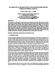
B. Graph Modeling The system monitoring data can be massive. For example, the data collected from a single computer system by monitoring the process interactions in one hour can easily reach 1 GB. Searching over such massive data is prohibitively expensive in terms of both time and space. Therefore, we devise a compact, graph-based representation that can greatly improve the performance of the detection procedure. The idea of compact graph design comes from our observation that the original system surveillance data is often largely redundant in several ways. First, the redundancy comes from the attributes, as each event record always contains not only the involved entities but also the attributes of these entities. Repeatedly storing the attributes of those entities in a large number of events introduce significant redundancy. Second, the redundancy comes from the events as the events that involve the same entities is always repeatedly saved (with different time stamps). Third, normally, the abnormal behaviors, such as intrusion attacks, complete in a short time window. Therefore, it is not necessary to search the data outside of the user-defined time window. {11:44:21} {09:16:24, 11:24:03}

grep

notebook.doc {08:21:13}

passwd

{09:25:01, 13:14:55}

{06:32:41}

ip1 -> ip2

dash INET

{11:51:52}

vim

{10:13:52}

{09:16:24, 11:24:03}

ud2

{10:05:02}

ud1

hosts {10:52:00} {07:02:14, 12:11:43}

https

{09:31:33}

Process

calendar.txt

UD

{06:16:21, 13:21:03}

index.html File

Fig. 2. An example of compact graph model; the red path corresponds to an abnormal event sequence

Our graph model eliminates redundancies in the data. Given the data in a time window, we construct a directed graph G =

(V, E, T ), with: (1) V as a set of vertices, each representing an entity. For enterprise surveillance data (see Section V-A), each vertex of V belongs to any of the following four types: files (F ), processes (P ), UDSockets (U ), and INETSockets (I), namely V = F ∪ P ∪ U ∪ I; (2) E as a set of edges. For each pair of entities (ni , nj ), if there exists any system event between them, we construct an edge (vi , vj ) in the graph, where vi (vj ) corresponds to ni (nj ); and (3) T as a set of time stamps. For any edge (vi , vj ), it is possible that it is associated with multiple timestamps (i.e., the corresponding event happens multiple times). We use T (vi , vj ) to denote the set of time stamps on which this event has ever happened. Formally, T (vi , vj ) = {e.t|e ∈ E, vi = e.nb and vj = e.nd }. nb (nd ) is the source (destination) entity of e. Given an event sequence of length ℓ, there is a corresponding path in G that includes ℓ vertices. In the rest of the paper, we will use event sequence and path interchangeably. In this paper, we are interested in only those event sequences that happen within a given time interval, namely the timespan is less than or equal to ∆t, where ∆t is a given threshold. In other words, the graph only records events that happen in a time window of size ∆t. Figure 2 shows an example of the compact graph for enterprise surveillance data. Note that according to the types of entity interactions that are allowed in UNIX (Section V-A), G is not a complete graph. Instead, it only allows the edges between (1) process and file nodes, (2) process and process nodes, (3) process and socket (both UDSockets and INETSockets) nodes, and (4) UDSocket and UDSocket nodes. By removing the redundancy of attributes and events, our graph representation can significantly compress the original heterogeneous event data while preserving relevant information for intrusion detection. Our experiment results in Section V-E demonstrate that the graph model reduces the space cost significantly. C. Path Pattern Generation The graph constructed by the graph modeling component can be densely connected. Path search in such graphs can be time costly. To speed up the path searching procedure, GID allows users to embed the predefined set of valid path patterns B first. The path patterns could be defined by the experts according to their experiences and knowledge. Arguably, it would be valuable to incorporate experts’ knowledge into the path pattern generation. Formally, given a graph G(V, E, T ), a path pattern B is of the format {X1 , . . . , Xℓ ), where each Xi (1 ≤ i ≤ ℓ) is either a specific entity (e.g., file install.log) in V or a specific entity type (e.g., P , which can be mapped to any system process). The length of B that consists of ℓ nodes is ℓ. Take the information leakage problem in computer systems for example, we set each Xi (1 ≤ i ≤ ℓ) as a specific system entity type, i.e., Xi ∈ {F, P, U, I}. Note that for all the paths that correspond to information leakage, they must satisfy that X1 = F and Xℓ = I.

Given a path p ∈ G and a path pattern B of G, let p[i] and B[i] represent the i-th node in p and B respectively, we say p is consistent with B, denoted as p ≺ B, if: (1) p and B have the same length; and (2) for each i, p[i] ∈ B[i] (i.e., the specific entity p[i] belongs to the entity type B[i]), we say B is a valid path pattern if there exists at least one path p in G s.t. that p ≺ B. For example, the path patterns of length 3 with the four entity types for information leakage problem are {F, F, I}, {F, P, I}, {F, U, I} and {F, I, I}. But the only valid one is {F, P, I}, because only a process node can connect a file node to a INETSocket node. In this way, we can extract all the valid patterns from B by searching in G. D. Candidate Path Searching Based on the valid path patterns B, the candidate path searching component searches for the paths in G that are consistent with B. Formally, given a set of path patterns B, the candidate path searching component aims to find the set of candidate paths C: C = {p|p ∈ G, ∃B ∈ B s.t. p ≺ B}.

(1)

Besides the consistency requirement, we also impose the following time order constraint on the search procedure, demanding that for each path that is consistent with B, its corresponding event sequence must follow the time order. Formally, a path p = {n1 , . . . , nr+1 } satisfies the time order constraint if ∀i ∈ [1, r − 1], there exists t1 ∈ T (ni , ni+1 ) and t2 ∈ T (ni+1 , ni+2 ) such that t1 ≤ t2 . This condition enforces the time order in the corresponding event sequences. A straightforward approach to find all candidate paths is to apply the path patterns and time order constraints to the breadth-first search algorithm. If no valid path patterns are provided, GID would only apply the time order constraints. One scan of the system event graph G is sufficient to find all candidate paths. We omit the details here due to the limited space. E. Suspicious Path Discovery It is possible that some candidate paths discovered by the candidate path searching component are not associated with abnormal event sequences. Hence it is necessary to distinguish the suspicious paths that are highly likely to be associated with abnormal event sequences among a large set of candidate paths. A straightforward idea of the suspicious path discovery is to define their anomaly based on the frequency of the system entities that are involved. Those paths that involve rarely-used system entities are considered as suspicious. This is not correct as many intrusion attacks indeed only involve system entities that are popularly used in many events. Consider the enterprise surveillance graph in Figure 2 as an example. The red path shows a typical insider attack, via which the secret passwd file is leaked through the vim and httpsd entities. Apparently vim is the editor process and the httpsd process is a background daemon process that supports https service. Both entities are

involved in many normal system events. The frequency-based anomaly approach cannot catch such intrusion attacks. Continuing the example, we notice that, however, the interaction between vim and passwd entities is abnormal, as typically the passwd file is accessed by the processes such as bash, but not by the vim process, which mainly serves as a file editor. Therefore, our basic idea is to define the anomaly based on both the system entities and the interactions among them. Each path is assigned an anomaly score that quantifies the degree of anomaly. Next, we discuss how to calculate the anomaly scores. First, we assign each system entity two scores, namely, a sender score and a receiver score. The sender (receiver, resp.) score measures the amounts of information that is sent (received, resp.) by the entity. For instance, the /etc/ passwd file has a high sender score but relatively low receiver score, as it is sent to many processes for access permission check, but it is rarely modified. In contrast, the /var/log/install.log file has a high receiver score. Both sender and receiver scores are computed by performing random walk on the system event graph G. In particular, given the graph G, we produce a N ∗ N square transition matrix A, where N is the total number of entities, and A[i][j] = prob(vi → vj ) =

|T (vi , vj )| , N P |T (vi , vk )|| |

(2)

k=1

where T (vi , vj ) denotes the set of time stamps on which the event between vi and vj has ever happened. Intuitively, A[i][j] denotes the probability that the information flows from vi to vj in G. We denote A as P F I U P →F P →I P →U P 0 A A A , (3) 0 0 0 A = F AF →P I AI→P 0 0 0 U→U U AU→P 0 0 A

where 0 represents a zero sub-matrix. Note that the non-zero sub-matrices of A (Equation 3) only appear between processes and files, processes and sockets, as well as UDSockets and UDSockets, but not between processes, because the interaction between process and process does not come with information flow. This is what is allowed by the Unix system. The calculation of sender and receiver scores is adapted from the reasoning of authorities and hubs [15]. In particular, let x be the sender score vector, with x(vi ) denoting the node vi ’s sender score. Similarly, we use y to denote the receiver score vector. To calculate each node (entity)’s sender and receiver scores, first, we assign initial scores. We randomly generate the initial vector x0 and y0 and iteratively update the two vectors by the following  T T xm+1 = A ∗ ym , (4) T = AT ∗ xTm ym+1

where T denotes the matrix transpose. According to Equation 4, an entity vi ’s sender score is the summation over the receiver scores of the entity to which vi sends information to. The intuition is that if an entity sends information to a large number entities of high receiver scores, this entity is an important information sender, and it should have a high sender score. Similarly, an entity should have a high receiver score if it receives information from many entities of high sender scores. As a result, an entity vi ’s receiver score is calculated by accumulating the sender scores of the entities from which vi receives information. From Equation 4, we derive  T xm+1 = (A ∗ AT ) ∗ xTm−1 . (5) T T ym+1 = (AT ∗ A) ∗ ym−1 In Equation 5, we update the two score vectors independently. It is easy to see that the learned scores xm and ym depend on the initial score vector x0 and y0 . Different initial score vectors lead to different learned score values. It is difficult to choose “good” initial score vector in order to learn the accurate sender and receiver scores. However, we find an important property in matrix theory, namely the steady state property of the matrix [10], to eliminate the effect of x0 and y0 on the result scores. Specifically, let M be a general square matrix, and π be a general vector. By repeatedly updating π with T T πm+1 = M ∗ πm , (6) there is a possible convergence state such that πm+1 = πm for sufficiently large m value. In this case, there is only one unique πn which can reach the convergence state, i.e., πnT = M ∗ πnT .

(7)

The convergence state has a good property that the converged vector is only dependent on the matrix M , but independent from the initial vector value π0 . Based on this property, we prefer that the sender and receiver vectors can reach the convergence state. Next, we discuss how to ensure the convergence. To reach the convergence state, the matrix M must satisfy two conditions: irreducibility and aperiodicity [10]. A graph G is irreducible if and only if for any two nodes vi , vj ∈ V , there exists at least one path from vi to vj . The period of a node v ∈ V is the minimum path length from v to v. The graph’s period is the greatest common divisor of all the node’s period value. A graph G is aperiodic if and only if it is irreducible and the period of G is 1. As our system event graph G is not always a strongly connected graph, the iteration in Equation (5) can not reach the convergence state. To ensure convergence, we add a restart matrix R, which is widely used in random walk on homogeneous graph [21] and bipartite graph [22]. Typically, R is a N ∗ N square matrix, with each cell value be N1 . With ¯ R, we get a new transition matrix A: A¯ = (1 − c) ∗ A + c ∗ R,

(8)

where c is a value between 0 and 1. We call c the restart ratio. With the restart technique, A¯ is guaranteed to be an irreducible and aperiodic matrix. By replacing A with A¯ in Equation (5), we are able to get the converged sender score vector x and receiver score vector y. We can also control the convergence rate by controlling the restart rate value. Our experiments show that the convergence can be reached within 10 iterations. Given a path p = (v1 , . . . , vr+1 ), based on the sender and receiver score, the anomaly score is calculated as Score(p) = 1 − N S(p),

(9)

where N S(p) is the regularity score of the path calculated by the following formula: N S(p) =

r Y

i=1

x(vi ) ∗ A(vi , vi+1 ) ∗ y(vi+1 ),

(10)

where x and y are the sender and receiver vectors, and A is calculated by Equation 3. In Equation (10), x(vi )∗A(vi , vi+1 )∗ y(vi+1 ) measures the normality of the event (edge) that vi sends information to vi+1 . Intuitively, any path that involves at least one abnormal event is assigned a high anomaly score. Consider the example of the suspicious path (the red path) in Figure 2. As the passwd file is rarely accessed by the vim process, the information transition probability between passwd and vim is low. Therefore, the event sequence is assigned with a high anomaly score. For each path p ∈ C, we calculate the anomaly score by Equation 9. However, it is easy to see that longer paths tend to have higher anomaly scores than the shorter paths. To eliminate the score bias from the path length, we normalize the anomaly scores so that the scores of paths of different lengths have the same distribution. Let T denote the normalization function. We use the Box-Cox power transformation function [20] as our normalization function. In particular, let Q(r) denote the set of anomaly scores of r-length paths before normalization. For each score q ∈ Q(r), we apply  qλ −1 : λ 6= 0 λ (11) T (q, λ) = log q : λ = 0

¯ λ) = 1 Pn T (qi , λ). where T (q, i=1 n To minimize the margin between the normalized and the normal distribution, we find the λ that maximizes the loglikelihood. A possible solution is to take derivatives of L(Q, λ) on λ, and pick λ that makes ∂L ∂λ = 0. The suspicious path discovery component returns those paths of top-k normalized anomaly scores as suspicious paths. F. Suspicious Path Validation To further validate the discovered suspicious paths, we calculate the t-value between the two groups of paths: all candidate paths C, and the set of discovered suspicious paths S. The t-test returns a confidence score that determines whether the difference between the two sets of paths is significant. If the confidence score is greater than 0.9 with p − value smaller than 0.05, all paths in S are considered as abnormal paths that are relevant to intrusion attacks. Otherwise, we treat those paths as normal and do not raise alerts. The suspicious path validation component prevents GIDfrom sending false alarms when there is no attack at all. IV. O PTIMIZED S USPICIOUS PATH D ISCOVERY

The suspicious path discovery method (Section III-E) calculates the anomaly score for each candidate path. However, the number of candidate paths can be prohibitively large. It would be desirable if we only need to check a small number of candidate paths to find those suspicious ones. In this section, we devise an optimization scheme that addresses this issue by integrating the threshold algorithm [30] with our intrusion detection algorithm. The optimization scheme notably improves the efficiency of suspicious path discovery (see Section V-C). Intuitively, the top-k suspicious paths are those candidate paths with the k largest anomaly score Score(p). We observe that the anomaly score function has the monotone property. In particular, given two paths p and p′ of the same length, ′ where p = (v1 , . . . , vℓ+1 ), and p′ = (v1′ , . . . , vℓ+1 ), if x(vi ) ≤ ′ ′ x(vi ) and y(vi ) ≤ y(vi ) for i ∈ [1, ℓ + 1], it must be true that N S(p) ≤ N S(p′ ), thus Score(p) ≥ Score(p′ ). Based where λ is a normalization parameter. Different λ values on the monotone property, we design the procedure shown in yield different transformed distributions. Our goal is to find Algorithm 1 to find the top-k suspicious paths, without the the optimal λ value to make the distribution after normalneed to calculate the anomaly score of each path. ization as close to the normal distribution as possible (i.e., Our algorithm is adapted from the well-known threshold T (Q, λ) ∼ N (µ, σ 2 )). algorithm [30]. First, we apply random walk on the graph G Next, we discuss how to compute the optimal λ. First, we to calculate the two vectors x and y. Second, for each type of assume that such λ exists to make T (Q, λ) ∼ N (µ, σ 2 ). The entities, we create two queues sorted in the descendent order density of a normalized scores is of the sender score and the receiver score respectively. Also, exp(− 2σ1 2 (T (q, λ) − µ)2 ) we sort the edges according the probability A[i][j]. After that, √ . (12) P rob(T (q, λ)) = in each iteration of the WHILE loop, we fetch the entity or 2πσ edge with the smallest score from each queue, and identify all The profile logarithm likelihood of the normalized distributhe valid paths that contain these entities and edges. Assume tion is that there is a path p consisting of these entities and edges, n n ¯ λ))2 X X (T (qi , λ) − T (q, n log qiwe , calculate Score(p). Apparently Score(p) is the highest )+(λ−1) L(Q, λ) = − log( 2 n anomaly score for all the paths that are not explored yet. If i=1 i=1 (13) Score(p) is no larger than the minimum anomaly score of all

Algorithm 1 Discover top-k suspicious paths Require: G = (V, E, T ), where V = F ∪ P ∪ U ∪ I, k, Ensure: SP that contains the top-k suspicious paths of G. Initialize SP as an empty priority queue; Apply random walk on G to calculate sender score vector x and receiver score vector y; Let FX be the files sorted in descendent order of the sender score. Let FY be the files sorted in descendent order of the receiver score. Create PX , PY , UX , UY , SX and SY in the same way. Let E ′ be the edges sorted descendingly by A[i][j] while PX , PY , UX , UY , SX , SY and E ′ are not empty do fx = FX .pop(), fy = FY .pop() px = PX .pop(), py = PY .pop() ux = UX .pop(), uy = UY .pop() sx = SX .pop(), sy = SY .pop(), e = E ′ .pop() Assume p is the path involving fx , fy , px , py , ux , uy , sx , sy , e ′ . if Score(p) ≤ min{Score(p′ )|p′ ∈ SP } then break else Find the path set P such that every path p confirms to the event sequence pattern and time constraint, and p involves at least one node in {fx , fy , px , py , ux , uy , sx , sy } or e′ . for all p ∈ P do if Score(p) > min{Score(p′ )|p′ ∈ SP } then Insert p into SP if SP contains k + 1 paths then Remove the (k+1)-th path from SP . end if end if end for end if end while return SP

paths in the output SP , we stop the iterations and output SP . Otherwise, we discover the paths P that involve at least one un-checked entity that is of the highest score in any queue, and calculate the anomaly scores of these paths. Let the kth path pk ∈ SP be the path in SP that is of the minimal anomaly score. For any path p ∈ P such that Score(p) > Score(pk ), we replace pk with p. By Algorithm 1, we only need to calculate the anomaly score for a small number of valid paths to find the top-k suspicious paths. It has proven that the threshold algorithm can correctly find the top k answers if the aggregation function is monotone [30]. Therefore, our optimization algorithm can find exact top-k suspicious paths efficiently. In Algorithm 1, we use random walk with restarts to calculate the sender and receiver scores. The complexity of the random walk step is O(N 2 ) [31], where N is the number of entities in the graph. This is because it only needs a constant

number of steps of matrix multiplication to converge. Suppose that there are C candidate paths, the time complexity to extract the top-k suspicious ones is O(C), as in the worst case, we need to calculate the anomaly score for every candidate path. Thus, the total complexity for Algorithm 1 for the worst case is O(N 2 + C). However, due to the early stop condition of the threshold algorithm, the average-case complexity of Algorithm 1 is O(N 2 + C ′ ), where C ′