Graph-based representations of point clouds - imati-cnr

Graph-based representations of point clouds Mattia Natali, Silvia Biasotti, Giuseppe Patan`e, Bianca Falcidieno Istituto di Matematica Applicata e Tecnologie Informatiche Consiglio Nazionale delle Ricerche Via De Marini 6 16149 Genova, Italy

Abstract This paper introduces a skeletal representation, called Point Cloud Graph, that generalizes the definition of the Reeb graph to arbitrary point clouds sampled from m-dimensional manifolds embedded in the d-dimensional space. The proposed algorithm is easy to implement and the graph representation yields to an effective abstraction of the data. Finally, we present experimental results on point-sampled surfaces and volumetric data that show the robustness of the Point Cloud Graph to non-uniform point distributions and its usefulness for shape comparison. Keywords: Graph-based representations, point clouds, shape abstraction, shape comparison.

1. Introduction Shape representation from data samples is a well known problem in many fields of science and engineering. In most of cases, the data samples are assumed to approximate a manifold embedded in a higher-dimensional space. A typical example is shape reconstruction from range images obtained by scanning real 3D objects: here, the dimension of the embedding space is three (i.e., the dimension of the Euclidean space) while the intrinsic dimensionality of the surface is two. Generally, point sets are supposed to densely sample the boundary of a smooth surface, which is reconstructed through moving least-squares [4, 6, 41], implicit [1] and Voronoi/ Delaunay [5, 29] approximations. Since point sets are able to represent arbitrarily complex 3D shapes without needing the explicit storage of the manifold connectivity, they have become a surface representation alternative to polygonal meshes and have been widely used for several applications. Among them, we mention ray tracing [2], surface reconstruction [43, 68], sampling [4], simplification [52], segmentation [8], spectral analysis [51], machine learning [12, 62], progressive rendering and streaming [33] Since only few works address the problem of computing high-level representations [14] of point clouds, this paper tackles the problem of defining graph-based representations of point clouds. By skeletal representation we mean an explicit graphlike coding of the essential structure of the shape underlying the input point cloud and the way the shape components glue together to form the whole. In general, a skeletal representation yields a compact and expressive shape abstraction, which attempts to reflect the human intuition. The use of sufficiently concise, informative, and easily computable skeletal representations, instead of the whole models, may facilitate the comparison process. In fact, Preprint submitted to Elsevier

the search in a database for an object similar to a query can be nearly impossible if approached by simply comparing point clouds or bulks of thousand triangles. Important aspects that drive the definition of a skeletal representation are the invariance to translations, rotations, and scalings; the identification and abstraction of shape features; the independence of the representation with respect to the shape embedding and discretization; the property of being medial with respect to the shape. From a general perspective, two main philosophies drive the definition of skeletal representations on triangulated surfaces: (i) defining a medial structure representation that always falls inside the shape and is equidistant from the shape boundary at each point or (ii) explicitly representing how the basic components of the shape are glued together to form the whole. We highlight that in the latter case, the skeletal representation is not necessarily medial with respect to the shape. Main examples of medial representations are: the Medial Axis [19, 20, 58], which in 3D may contain both curve segments and sheets with non-manifold connections; the medial curves computed through segmentation [22, 25, 39]; the medial geodesic skeleton [30]; the mesh contraction based on Laplacian smoothing [9] and surface-based operations [3, 26, 60]. As a representative of the second class of skeletal representations, the Reeb graph [54] codes the evolution and arrangement of the level sets of a real function f : M → R, defined over a manifold M. The Reeb graph has been proven to be always a 1-dimensional complex and in its original definition provides a description that is not invertible. This means that the input shape cannot be exactly recovered from the Reeb graph and the geometric information stored in its nodes and arcs. Since the Reeb graph is parametric with respect to the input map, changing f induces different descriptions of the same surface, which can be tackled to shape comparison [38], segmentation [13], and visualization [63]. Examples of functions effectively used February 9, 2011

(a)

(b)

(c)

(d)

Figure 1: (a-d) Graph representations of several point-sampled surfaces with different features and sampling densities. The original triangle mesh representing the model in (a) has 11 components.

in applications are geodesic distances, harmonic and Laplacian eigenfunctions. Efficient algorithms for the computation of the Reeb graph exist for polyhedral surfaces [24, 50], volume models [63], and higher dimensional data [49, 32, 37]. A main limitation of the aforementioned approaches is that they assume a manifold connectivity for the representation of the input shape, thus making skeletons unavailable for nonmanifold models, such as triangle soups and point sets in arbitrary dimension. Concerning point sets, the main approaches for skeletal representations are based on medial-like concepts and exploit the identification of a rotational symmetry axis [61] through symmetry detection; the Voronoi diagrams [47]; a thinning process based on the 1D moving least-squares construction [40]; a Laplacian-based contraction [21]; and the maximal spheres inscribed inside the input point set [56]. Methods that approximate the Medial Axis generally assume that the point cloud densely samples the external surface of a solid [5, 28]. A few methods generalize the Reeb graph to point clouds, either using the level sets of geodesic distance functions and a discrete Reeb graph coding [67, 65] for human body scans, or introducing a cluster-based multi-resolution structure, which may admit input functions of co-dimension higher than one [59].

function f makes the Point Cloud Graph suitable for several applications (e.g., shape abstraction, sketching, comparison). Replacing the level sets with strips leads to a robust computation of the skeletal curve when P has deficiencies in terms of noise, missed data, and multiple components. Additionally, this choice avoids the need of computing the moving least-squares surface underlying P and allows us to extract the skeleton of an arbitrary set of points in Rd , without requiring a local smoothness or connectivity of the underlying shape. Finally, in R3 the Point Cloud Graph reduces to the Reeb graph of the underlying manifold as the point cloud becomes denser. Fig. 1 shows the results of the proposed algorithm on point-sampled surfaces. The main contribution of the proposed approach relies on its generality with respect to (P, f ) and the capability of handling point sets in any dimension. Concerning the first contribution, our computation of the Point Cloud Graph handles shapes that are not necessarily described as an assembly of cylindrical patches and joints as in [61]; is restricted neither to point sets representing 0-genus surfaces nor to a specific scalar function; does not use any template to drive the graph extraction, as in [65] for human scans. Finally, we directly compute the skeletal representation without a graph post-processing, which is generally required by the Laplacian-based contraction [21]. According to the definition of the Reeb Graph [54], the Point Cloud Graph codes a point set P in a 1D representation, whose properties depend on those ones of f and the shape underlying P. Note that reducing the width of the partition of the interval containing the image of f forces the strips to converge to the corresponding level sets. Even though the Point Cloud Graph cannot be used to exactly recover the input data (invertibility property), the graph is useful to compute an approximation of the input point set through an implicit representation Σ := {p : F(p) = 0} with radial basis functions [61]. Concerning the computation of the Point Cloud Graph for higher dimensional data, the proposed approach remains unchanged by substituting surface with volume strips. The Point Cloud Graph, as well as the Reeb graph, does not distinguish all the features in higher dimensions [16]; in fact, in case of volumetric data it may not code cavities. Since the Point Cloud Graph is intended to generalize the Extended Reeb graph to point clouds embedded in Rd , differently from [59] we consider

Overview and contribution. This paper introduces a skeletal representation, called Point Cloud Graph, which generalizes the definition of the Reeb graph to arbitrary point clouds sampled from m-dimensional manifolds embedded in the d-dimensional space. The input point sets represent single shapes, scenes with several objects, and volumetric data, without assumptions on the quality of the input point sets in terms of noise, missing data, and low sampling densities. The proposed approach computes the Point Cloud Graph of the point set P := {pi }ni=1 ⊆ Rd by joining the connected components of strips of a real function f : P → R. To extract this skeletal representation, we exploit the local connectivity of the k-nearest neighbor graph of P, which is also used to identify the connected components of P (P may represent a set of shapes) and of the strips of P induced by f . Intuitively, the Point Cloud Graph codes the points according to their nearness but it might distort large scale distances. This is a desirable property in those applications where large scale distances carry a little meaning. Moreover, the flexibility of the choice of the 2

Figure 3: Connectivity between two point sets P and Q.

which contains the elements of Ikpi whose distance from pi is equal to or lower than τ (Fig. 2). These different types of neighbors will be used to extract the connected components of the strips and join the corresponding nodes of the graph without meshing the point set (Fig. 3). To this end, we adopt the following notions of connectivity and connected components of point sets.

Figure 2: Example of k-nearest neighbor Ikp , which includes the k points of P k closest to p; Ik,r p is the set of points in Ip whose distances from p are lower than r.

only R as co-domain of the function f and we do not admit the overlap between clusters of points. Admitting overlapping domains would not be meaningful for the equivalence relation in Definition 2.2. Furthermore, in R3 the number of loops of the corresponding Reeb graph would be no more equal to the genus of the input surface. The paper is organized as follows. In Section 2, we provide formal definitions of the point cloud connectivity, introduce the notion of Point Cloud Graph, and detail our graph extraction technique. In Section 3, we present our experimental settings, discuss the robustness of the method with respect to noise and parameters, and show shape matching as a possible application. Conclusions and future developments are provided in Section 4.

Definition 2.1. Let P := {pi }ni=1 and Q := {q j }mj=1 be two point sets. Given a positive threshold τ, P and Q are τ-connected if exist two points pi ∈ P and q j ∈ Q such that ||pi − q j ||2 ≤ τ. In particular, a point set P is said τ-connected if each nonempty subset Ω of P and its complementary set ΩC in P are themselves τ-connected. Then, a connected component of a point set P is a τ-connected set of points in P. Finally, given two τ-connected components C1 and C2 we define their distance d(C1 , C2 ) as d(C1 , C2 ) = min ||p1 − p2 ||2 . (1) p ∈C 1 1 p2 ∈C2

2.2. Graph definition

2. The Point Cloud Graph

We now generalize the Reeb graph definition to scalar funcOur graph representation broadens to point sets concepts tions defined on point sets. Given the scalar function f : P → related to the Reeb graph; in particular, it generalizes the ExR, we denote its minimum and maximum with tended Reeb graph (ERG) originally defined on triangle meshes [15] and the Discrete Reeb graph [67]. We name this new represenvm := min { f (pi ), pi ∈ P}, v M := max { f (pi ), pi ∈ P}, i=1,...,n i=1,...,n tation Point Cloud Graph (PCG). Similarly to the ERG, the aim of the method is to extract the PCG of the pair (P, f ), where and Im( f ) = [vm , v M ] is the interval of R that contains the disP := {pi }ni=1 ⊆ Rd is a set of points in Rd and f : P → R is a crete image Im( f ) := { f (pi ), pi ∈ P} of f . For any interval scalar function defined on P, i.e., f (pi ) is known for each point [a, b], a < b, contained in Im( f ), the discrete strip related to pi ∈ P. The idea behind our approach is to organize the data [a, b] (Fig. 4(a)) is defined as the set S[a,b] = {pi ∈ P : a ≤ into a family of strips of points of P, to associate a node to each f (pi ) ≤ b}. Then, we replace the role of contours in the definiconnected component of the strip, and to insert an arc between tion of the Reeb graph [54] with the concept of strips. two nodes if their distance is less than a user given threshold. In the following, we introduce the connectivity among the Definition 2.2. Let f : P → R be a real-valued function depoints of P (Section 2.1), the definition of the Point Cloud fined on a point cloud P and J = {J1 , . . . , Jm } be a partiS Graph of (P, f ) (Section 2.2), and its computation (Section 2.3). tion of Im( f ) by non-empty intervals, i.e. Im( f ) = m k=1 Jk , T Ji J j = ∅, i , j. Then, the Point Cloud Graph of P with 2.1. Connectivity and connected sets of point clouds respect to f and J is the quotient space of P × R defined from Within the k-nearest neighbor graph T of P, each point the equivalence relation “∼”: (p, f (p)) ∼ (q, f (q)) if and only pi ∈ P is associated to its k nearest points of P, which identify if ∃Jk ∈ J such that: the neighbor Ikpi := {p js }ks=1 of pi . In a similar way, the σ1. f (p), f (q) ∈ Jk ; nearest neighbor of pi is defined as the set of points of P that 2. p, q ∈ P belong to the same connected component of fall inside the sphere of center pi and radius σ. Finally, we SJk . introduce the neighbor k Ik,τ pi := {p j s ∈ Ipi : kpi − p j s k2 ≤ τ},

3

(a)

(b)

(c)

(d)

(e)

(f)

Figure 4: (a-d) Main steps of the proposed approach; as f , we consider a harmonic function with one maximum and one minimum. (a) A strip (red) and (b) its connected components are identified with different colors. (c) The nodes of the Point Cloud Graph are computed as centroids of each connected component and (d) linked to form the arcs of the PCG. (e,f) PCG with respect to the height function oriented according to the y-axis. The same axis frame is used in the rest of the paper. In (e), the green nodes represent strips with more than one component and (f) the corresponding arcs are identified with three colors.

The connected components of a strip (Fig. 4(b)) correspond to its τ-connected sets defined in Section 2.1. In particular, we notice that Definition 2.2 introduces the PCG through an equivalence relation that requires the set J to be a partition. Indeed, the elements of J cannot intersect and the PCG cannot be implemented through the clustering strategy introduced in [59]. 2.3. Graph extraction To describe how our algorithm extracts the Point Cloud Graph as a couple G = (V, E), where V and E are respectively the set of the graph nodes and edges, we distinguish four fundamental steps: 1. choice of the scalar function f ; 2. extraction of the strips of f (Fig. 4(a)); 3. identification of the connected components of each strip (Fig. 4(b)) and creation of the set V of nodes (Fig. 4(c)); 4. generation of the set E of arcs (Fig. 4(d)).

and its closeness to the underlying surface. An alternative is to trace the shortest path among the nodes of an extended sphereof-influence graph. In this case, the Point Cloud Graph associated to the averaged geodesic distance from a set of source points is useful for the computation of bending invariant shape signatures [55, 65]. To define harmonic scalar functions on a point set P, the Laplace-Beltrami operator is discretized by the Laplacian matrix L := (Li j )ni, j=1 as [10, 11, 23]   −1    ai j /αi Li j :=     0

i = j, p j ∈ Npi , else,

    kpi −p j k22   , a := exp −  ij h2  P    αi := j∈Np ai j . i

We briefly remind that the vector h, h , 0, is an eigenvector of L related to the eigenvalue λ if and only if Lh = λh. Once L has been built, the computation of the harmonic scalar function resembles the case of triangle meshes [31, 34, 46]. Choosing a set of boundary conditions B := { f (pi ) = ai }i∈I , I ⊆ {1, . . . , n}, Choice of the scalar function f . The graph extraction scheme we solve the linear system L⋆ f ⋆ = b, where f ⋆ := ( f (pi ))i∈IC is can be applied to any map f defined on P, thus providing a set the vector of unknowns, IC is the complementary set of I, b is of characterizations and different descriptions of the shape una constant vector, and L⋆ is achieved by removing the ith -row derlying P. The properties of the corresponding skeleton will and ith -column of L, i ∈ I. reflect those of f , thus yielding to a multi-view shape descripThe Laplace-Beltrami eigenfunctions [12], or the heat kertion. Coding the PCG as an attributed graph, the choice of the nel [42], provide a family of maps whose Reeb graphs code function f influences the geometric and topological informathe features of P in a multi-scale manner; i.e., from global tion stored in its nodes and arcs. Scalar functions may be either to local levels of detail. Even though a general choice of f induced by the application context or intrinsically defined by does not guarantee that the corresponding Reeb graph is inthe manifold M underlying P. In the following, we briefly reside P, specific choices of the input maps such as the Laplaceview the computation of the geodesic, harmonic, and Laplacian Beltrami eigenfunctions provide representations that are cenfunctions. tered and well aligned with generalized cylinders of P (if any). Recent works [44, 55] on the computation of geodesics on a Furthermore, non-cylindrical joints are represented as graph edges point set P have enriched the class of scalar functions on P with without self-intersections. For shape analysis, we mainly focus geodesics-based maps, previously defined on triangle meshes [38] on functions that are intrinsically defined by the point cloud, and used for shape comparison [27, 45]. For instance, in [55] such as the Laplacian eigenfunctions. piecewise linear approximations of geodesic paths on pointExtraction of the strips of f . According to Definition 2.2, the sampled surfaces are computed by minimizing an energy funcstrips are extracted with respect to a partition {Jk }m tion, which takes into account both the geodesic path length k=1 of the in4

Table 1: Computational cost of the main steps of the proposed approach, where s is the number of source points used for the computation of the geodesic distance.

Task Load Function k-nearest neigh. graph Conn. components Arc constructions

Comput. cost O(n) O(n)-O(sn log n) O(n log n) O(kn) O(n)

(a)

Figure 5: The node ni1 is linked to node ni+1 1 . Similarly, there is an arc between i , Ci+1 ) > τ, we have not a linking edge between nodes ni2 and ni+1 . Since d(C 2 2 1 ni2 and ni+1 . 1

terval Im( f ) (Fig. 4(a)). The easiest way to partition Im( f ) into n s sub-intervals is to select n s + 1 values v0 := vm , v1 , . . . , vns := v M , vi ≤ vi+1 , and define each strip as SJi := f −1 (Ji ), Ji = [vi , vi+1 ), i = 0, . . . , n s − 1. This slicing strategy is quite common in the extraction of discrete approximations of the Reeb graph because uniform interval subdivisions of Im( f ) allow us to approximate the size and the relevance of a feature in terms of the length of the arcs of the graph; i.e., the longer the arc the more important the feature coded by the graph. Furthermore, it is possible to define an iterative sequence in the interval subdivision that makes the graph multi-resolutive. For more details on the slicing strategy, we refer the reader to [16, 38].

(b) Figure 6: Point Cloud Graph of a scene with (a) three and (b) four components. As scalar function, we have chosen the height function with respect to the zaxis.

are visited sequentially with respect to the increasing ordering of the corresponding intervals Ji . According to Equation (1), two connected components Cis and Cri+1 are linked if d(Cis , Cri+1 ) ≤ τ; in this case, we add the arc (nis , nri+1 ) to G (Fig. 4). The extraction of the set E of arcs ends when all the possible links among the connected components of two consecutive strips have been processed (Fig. 5). The construction of the arcs allows us to easily recognize branching parts. Figs. 4(d,e) show the Point Cloud Graph of the same point cloud with respect to two different functions. Differently from [57] and in order to extract the graph of scenes, which are typically composed of several components (Fig. 6), we do not automatically connect adjacent strips that have only one connected component. Finally, Figs. 7, 8, and 9 show the Point Cloud Graph of the same shape with different functions.

Connected components of strips and creation of the set V of nodes. Once we have identified the strip SJi , we detect its τconnected components with respect to Definition 2.1. To extract a τ-connected component Cij of the strip SJi , we select a point p j1 ∈ SJi that has not been marked as belonging to any τ-connected component. Then, all the points of SJi ∩ Ik,τ p j1 are marked as belonging to Cij and we recursively repeat this expansion on all the points of Cij . If at the end of this process there are points of SJi that are still unmarked, then we select one of them, identify a new connected component, and continue until all the points of SJi have been labeled as visited. The whole process is applied to all the strips and ends when each point of P has been assigned to some τ-connected component. Finally, we associate a node nij to every connected component Cij . As spatial representative of nij , we choose the centroid of Cij , (Fig. 4(c)).

Computational cost. Our algorithm is computationally efficient and handles point clouds with hundred thousands of points and more than one object. Analyzing the single steps of the algorithm (Table 1), the data loading requires O(n) operations, where n is the number of points of P. The computation of the input scalar function f varies from O(n) to O(n log n). For instance, the evaluation of the height function and the distance from the center of mass is linear in the number of points; the computation of the geodesic distance from s source points is O(sn log n) using the Dijkstra’s algorithm; and the solution of the Laplace-Beltrami eigenvalue problem is super-linear in n

Creation of the set E of arcs. According to Definition 2.2, the node nij , which codes the connected component Cij , must be linked to the nodes that correspond to the connected components of the strips SJi−1 and SJi+1 . Note that these strips {SJi }i 5

(a)

(b)

(c)

(a)

(b)

(c)

(d)

(e)

(f)

(g)

(h)

(d)

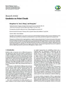
Figure 7: Point Cloud Graph of the same point cloud with respect to different scalar functions: (a) height function with respect to the z-axis; (b) f (p) := log(kpk2 + 1); (c) f (x, y, z) := x2 − y2 , p := (x, y, z); (d) f (p) := kpk2 .

Figure 9: Point Cloud Graphs of the scans of two statues with respect to (a,b,e,f) Laplacian-Beltrami eigenfunctions and (c,d,g,h) harmonic functions.

Figure 8: In (a), the graph is represented as two overlapping arcs. (b) Changing the scalar function, the arcs of the Point Cloud Graph are explicitly coded. Here, f is the height function with respect to (a) the z-axis and (b) y-axis.

our method to point sets with different sampling density, noise level, distribution of shape features, and missed parts. Most of point clouds corresponds to 3D scans of real models such as small statues and human bodies in different poses. We also consider point samples of volumetric data, i.e., where the underlying manifold is a 3−manifold with boundary embedded in R3 . For our tests, we have considered 50 points clouds from the AIM@SHAPE repository 1 , 30 body scans from the CAESAR Data Samples2 , and the 400 models of the SHREC 2007 benchmark3. The non-orientable models have been obtained from parametric samples of the Moebius surface and Klein’s bottle and the two scenes have been composed from objects of the data sets. To evaluate how the Point Cloud Graph depends on the data quality, the point clouds have been perturbed with geometric noise, by modifying the point coordinates. To show the scalability and the efficiency of the method (Table 2), the size of the data set ranges from a few thousand points to over one million. All the experiments have been performed over a mini-laptop equipped with Linux operative system, Mobile Intel Celeron 900MHz, and 2048MByte Ram. Beside the choice of the input function f , the arcs and nodes of the Point Cloud Graph are determined by the point cloud connectivity stored in the k-nearest neighbor graph. For point sets that represent 3D surfaces, we have experimentally verified that when the sampling of P is sufficiently dense the number of

and the number of eigenfunctions computed. The computation of the k-nearest neighbor graph T takes O(n log n) operations [7] and the creation of the strips is linear in n. For each strip, the computation of the connected components takes O(kn) operations. The extraction of the arcs of G requires to traverse two consecutive strips and visit their points at most twice; indeed, this step runs in O(n) operations. Finally, the overall computational cost is O(n)+O(n log n)+O(kn) = O(max{kn, n log n}), which does not considerably differ from the O(n log n) time required to compute the Reeb graph over triangle meshes [24, 16] and an efficient implementation of the clustering strategy in [59]. 3. Discussion and results Once our experimental settings have been introduced (Section 3.1), we discuss the main properties and degrees of freedom in the computation of the Point Cloud Graph; namely, the choice of the parameters (Section 3.2), its robustness (Section 3.3), the generalization to volume data and non-orientable surfaces (Section 3.4), and the application to shape comparison (Section 3.5). 3.1. Experimental settings To analyze the behavior of the Point Cloud graph with respect to the size of the neighbor of each point through the connectivity parameters introduced in Section 2.1, we have applied

1 http://shapes.aim-at-shape.net 2 http://www.hec.afrl.af.mil/HECP/Card1b.shtml#caesarsamples 3 http://watertight.ge.imati.cnr.it/

6

(a)

(b)

(c)

(d)

(b)

Figure 10: (a) The adaptive selection of the threshold τi allows us to better identify through holes in the point clouds as loops of the Point Cloud Graph. (b) The choice of a constant τ provides a skeleton that codes a lower number of local details. Here, f is the first non-trivial Laplacian eigenfunction.

Figure 11: Point Cloud Graph of a point set with (a,b) a low and irregular sampling density with missed parts (shoulder and feet in (b)), which are occluded during the acquisition process. (c,d) Zoom-in. For both examples, the extracted skeletal representations capture the main features of the underlying surface. In both cases, we have selected the first non-trivial Laplacian eigenfunction.

loops of the PCG is equal to the genus of the surface underlying P. Since the sampling density varies from model to model, it is crucial to automatically select a threshold that identifies the connected components of both the shapes of a scene and the strips of each building shape. To this end, we assume that the 3D shapes are coherently sampled, i.e., the local sampling density σP of P [53] is equal to or lower than the distance used to identify the connected components of the strips, the size of the through holes and the connected components.

variation of the sampling density occurs, the choice of τ j might provide problems for the identification of topological handles whose size is approximately τ j (Fig. 10). A crucial part for the extraction of G is related to the computation of the connected components of each strip and the generation of the arcs of the graph, where multiple components occur. These two steps of the algorithm are guided by the expansion radius τ j of the neighbor of each point of SJi . The tolerance τ that identifies the connected component of the strip SJi will be also defined as a multiple of τ j . The adaptive choice of the parameters is also crucial when we deal with scenes that include components with a different sampling density. For instance, in Fig. 6(b) the table model is denser than the other ones and the dog surface is not uniformly sampled. In case of a non-uniform distribution of points, the Point Cloud Graph could present more/less connections than expected or many connected components (Figs. 11 and 12). Fig. 12(a) shows how our representation automatically distinguishes spurious data, such as regions of the platform on which the human is standing during the body acquisition, from body parts partially occluded. Additionally, the rear part of the head is correctly connected to the main body. Table 2 summarizes the characteristics of the PCG in terms of number of elements, loops, and connected components with respect to different choices of k and τ. For the computation

3.2. Choice of the parameters Since the choice of the parameters τ and k is crucial to obtain an effective representation of the shape characteristics, we analyze how their choice influences the Point Cloud Graph and how to automatically determine them. To deal with nonuniform point samples or partially missing data, we introduce an adaptive definition of τ, which is iteratively tuned according to the local density of the point cloud P. To guarantee the coherence of the point cloud, we fix the value of τ1 as a multiple of σP and initialize the connected components of SJi . Then, during the expansion process and in a neighbor of a point p ji of the i−th strip SJi we iteratively refine the constant τ j+1 , j ≥ 1, as follows:  α j+1 + jτ j k,τ j    j+1 , |Ip ji | = k, τ j+1 :=  j   2α j+1 + jτ j , |Ik,τ p ji | < k, j+1

where |I| is the number of points of the set I and α j+1 = maxp∈Ik,τ j kp − p ji k2 . In those shape regions where an irregular pj

(a)

i

7

(a)

(a)

(b)

(c)

(d)

(e)

(f)

(g)

(h)

(i)

(j)

(b)

Figure 12: (a,b) Point Cloud Graph extracted from partially occluded body scans and in different postures. In these examples, we have selected the first non-trivial Laplacian eigenfunction.

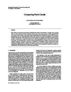
Figure 13: If the original point cloud (a) is perturbed with a Gaussian noise (be), then the number of nodes and arcs of the PCGs does not change. The PCGs in (f-h) correspond to the ones in (c-e) selecting ns = 30 instead of ns = 50. For (i,j), the reference Point Cloud Graphs are shown in Figs. 9(b,g), respectively. In these examples, the chosen scalar function is the height function in the z-axis direction.

of these graphs, the number of strips has been fixed to 30 for the bi-torus model, 100 for the hand model, and 50 for the 3D scene. Our tests have shown that if the parameters k and τ are arbitrarily chosen the number of loops of the graph may vary (e.g., Fig. 13). Moreover, the value τ j affects the connectivity of the graph: this is not surprising because when τ j increases the τ−connected sets become larger and the corresponding nodes are connected. In our data set, we have experimentally verified that a good compromise between computational complexity and efficacy of the description is to choose k smaller than 12; to initialize τ1 from 5 to 10 times σP ; and to set τ as 2τ j , where τ j the is the adaptive threshold previously discussed. If not differently specified in the text, then we set k = 10, τ1 = 5σP , and τ = 2τ j .

fact that we code the evolution of the strips instead of the contours, which are more sensitive to local perturbations of both P and f . As shown in Figs. 12 and 14, the Point Cloud graph handles either irregularly or partially sampled data, due to occlusions during the acquisition process. For instance, Fig. 12(a) shows the behavior of the graph with respect to shape outliers. In fact, this body scan presents a few points (low-left) that can be considered as noise. With our standard choice of the parameters k and τ j , the human model and few isolated points (left part) are abstracted as distinct graphs. The smallest component disappears only when the chosen parameter τ allows us to glue this small component to the body. Moreover, Fig. 14 depicts that, differently from [61], the flexibility in the choice

3.3. Robustness We now discuss the robustness of the graph to noise, local deformations, and missed data by experimentally verifying how these factors affect the corresponding structure. To this end, we simulate a geometric perturbation of the point cloud modifying the coordinates of the points through random Gaussian perturbations. The variance of noise perturbation of the models in Figs. 13(b-e) is 2%, 5%, 10%, and 15% of the maximum diameter of P, respectively. All these graphs have been obtained using n s = 50 strips. The overall structure of the graph is the same even if the number n s of strips varies: Figs. 13(f-h) show the PCGs extracted setting n s = 30 and the noise variance is equal to 5%, 10%, and 15%. Moreover, we notice that when the bitorus model is perturbed with a noise variation higher than 5% the corresponding triangle mesh is no more manifold and small self-intersections appear; indeed, we are not able to extract the Reeb graph from the mesh while this is possible with our PCG. Additional examples are depicted in Figs. 13(i,j): these models correspond to 2% noise perturbations of the ones in Figs. 9(b,g), respectively. In all cases, the extraction of the skeletal structure remains stable; i.e., the number and position of nodes and arcs do not significantly change. This property is mainly due to the

Table 2: Point Cloud Graph complexity. The variation of τ and k influences the connectivity of the graph in terms of number of connected components CC, vertices |V|, edges |E|, and loops. The Bi-torus, the Hand, and the Scene point clouds are respectively shown in Figs. 13(a), 1(d), and 6(a), respectively.

Model Bi-torus Bi-torus Bi-torus Bi-torus Bi-torus Hand Hand Hand Scene Scene Scene 8

n 12K 12K 12K 12K 12K 37K 37K 37K 330K 330K 330K

τ 2τ j 2τ j 10τ j 2τ j 2τ j 2τ j 2τ j 2τ j 2τ j 4τ j 10τ j

k 10 7 7 100 102 10 7 4 10 8 12

|V| 42 70 42 31 30 155 161 302 250 253 232

|E| 43 97 43 31 29 154 160 407 250 252 233

loops 2 18 2 1 0 0 0 106 3 3 3

CC 1 1 1 1 1 1 1 1 3 4 2

(a)

(c)

(b)

(d)

(e)

Figure 15: Point Cloud Graph of point sets sampled from (a) a Mobius surface, (b) a plane with three twists, and (c-e) a Klein bottle at different resolutions. In (a,b), the input map is the height function with respect to the y-axis. In (c-e), we have selected the first non-trivial Laplacian eigenfunction.

of the parameter τ automatically provides an estimation of the entity of the missed part. In fact, these examples represent a sequence of different samples of the same statue, whose resolution increases from (a) to (d). To compute the PCG, we have considered the distance from the center of mass and set the parameters k, τ1 , and τ with the default values discussed in Section 3.2. The graph in Fig. 12(a) highlights that the bust and the bottom of the statue is completely missing: this implies that a loop of the graph is broken and an additional loop appears in the bottom. The two intermediate PCGs in Fig. 12(b,c) are qualitatively and qualitatively equivalent while the PCG of a finer sample (Fig. 12(d)) of the statue correctly recognizes the two hands and has an additional loop.

Table 3: Statistics on the Point Cloud Graph extraction for some of our test models, the last four rows refer to point clouds of volumetric data: n number of points of P, nS number of strips used to extract the description, |V| cardinality of the set of nodes, |E| number of arcs of G. Time is expressed in seconds.

Model Monk - 11(a) Camel - 1(c) Hand - 1(d) Ippocrates - 10(a) Human - 11(b) Scene - 6(a) Raptor - 1(a) Hand - 16(a) Vertebrae - 16(b) Skull - 16(c) Ear - 16(d)

3.4. Non-orientable surfaces and volume data In the following, we show that our approach is able to describe a class of data larger than the Reeb graph, including point clouds originated by surfaces, volume data, or m−dimensional manifolds embedded in Rd with multiple components. For instance, since the original triangle mesh representing the model in Fig. 1(a) contains 11 components, it is not possible to compute the Reeb graph directly on the triangle mesh while our algorithm effectively runs also on this example. The same remark holds for the representation of sets of objects as in case of scenes (Fig. 6). Our graph representation also handles point sets representing non-orientable surfaces (Fig. 15) and volume data (Fig. 16), without building a manifold representation of the model. In all these examples, the values of k and τ are the default ones ex-

n 30K 35K 53K 102K 190K 330K 1M 29K 17K 38K 153K

nS 120 140 100 200 120 200 400 30 20 50 20

|V| 137 241 221 222 249 1003 1164 49 20 65 60

|E| 141 242 220 226 248 1003 1142 48 19 65 92

Time 1,2 1,7 4,1 11,9 41,8 370 435 5 3 5 221

cept for the models in Fig 15(c-e) (τ = 10τ j ) and Figs. 15(c-e) (k = 25, k = 15, k = 30). Volume data are quite common in medical and FEM applications. Until now, the extraction of the Reeb graph description for these data required the generation of a tetrahedral representation of P [49] and the identification of hole cuts [63] to have computational efficiency. In its original definition, the Reeb graph is not able to fully represent cavities, similarly the PCG has the same limitation. For instance, in Figure 16(c) the skull cavity is simply represented with a sequence of nodes and arcs. Table 3 reports statistics on the Point Cloud Graph computation for 3D shapes with different sampling den9

(a)

(a)

(b)

(c)

(d)

(b)

(c)

Figure 16: (a-d) Point Cloud Graph of volume data. Here, the map is the height function with respect to the main direction provided by the Principal Component Analysis on the input data set. According to the definition of Reeb graph, (a) highlights a situation for which the choice of f generates a PCG which is not medial to the shape.

(d)

Figure 14: (a-d) Point Cloud Graph with respect to irregular sampling density and missed part. Slightly increasing the shape resolution improves the quality of the Point Cloud Graph, in terms of a lower number of terminal arcs and a better alignment with the underlying shape. Here, the height function is in the direction of the z-axis.

D is a pseudo-metric, which satisfies positivity, symmetry and triangle inequality; identity is not verified (i.e., D(G1 , G2 ) = 0 ; G1 ≃ G2 ). More details can be found in [48]. In our tests, we have selected seven classes (human, cup, table, glass, octopus, plier, and bird models) from the SHREC 2007 benchmark on watertight models [35] and tested the retrieval performance of the Point Cloud Graph using the first and second non-trivial Laplace-Beltrami eigenfunctions, either singularly or in combination. Table 4 quantitatively compares the distances between couples of models (three humans, two cups, and two tables) computed either using the PCG (bottom value) or the Reeb graph (top value) as shape signatures. Despite the relative relevance of the numerical scores, the values of the distances are nearly comparable and in both cases well discriminate among objects belonging to different classes. A qualitative comparison of the two descriptors is shown in Fig. 17, where the precision-recall diagrams of the PCG and the Reeb graph (RG) [48] are depicted over the benchmark and the human model class. Again, these diagrams confirm that the performance of the two descriptors is substantially the same; in fact, in our feeling the relevance of the PCG graph is in the extension of the application domain (more objects, even disconnected and polygon soups) rather than one more method that slightly improves graph matching using Reeb graphs.

sities and resolution. 3.5. Shape comparison A current limitation of the use of the Reeb graph for matching purposes is that the existing algorithms [17, 64, 18] and applications to relevance feedback [36] requires the models to be watertight and without topological artifacts (e.g., dangling edges, multiple components). Indeed, the use of the Reeb graph is limited to a narrow number of data sets. In this context, we outline how the graph matching techniques used for Reeb graph comparison is easily adapted to the Point Cloud Graph, thus broadening the use of this description to quite a number of data sets. In our experiments, we compare the Point Cloud Graphs using the graph distance [48], which is an extension to set of graphs of Laplace-based metric [66], and match both single or sets of graphs. More formally, we consider the set of elementary symmetric polynomials: X vi1 vi2 · · · vi j , j = 1, . . . , n. S j (v1 , . . . , vn ) = i1