Graph coloring algorithms for fast evaluation of curtis ... - CiteSeerX

12.3

GRAPH COLORING ALGORITHMS FOR FAST EVALUATION OF CURTIS DECOMPOSITIONS Marek Perkowski, Rahul Malvi, Stan Grygiel, Mike Burns, and Alan Mishchenko Portland State University, Department of Electrical and Computer Engineering, Portland, Oregon, 97207-0751, USA

mperkows @ee.pdx.edu Abstract

F as follows: F ( X ) = H ( G ( B ) , A )where functions G , H , F can be all multi-output. Set of input variables X is first partitioned to the set of bound variables B and the set of free variables A (sets A and B can overlap in the so-called "non-disjoint decompositions", then sets A and B are formally a cover of set X, we will keep the name partition for uniformity). The set of bound variables is called the bound set and the set of free variables is called the free set. There exist some methods to find set PAR of good partitionings of set X to sets A ; and Bi [22], but they are not a subject of this paper. Then each set ( A ; , B j ) is tested for decomposition, For some of these subsets (Ai,B;) there exist decompositions, for some other there are no Curtis decomposition. Some of the existing decompositions are also evaluated as better than others using certain cost functions. When the set ( A , , B , ) is found'that its corresponding decomposition is evaluated as having the smallest cost for all subsets of PAR, functions C, and H j are actually created from F . This two-level decomposition process is next recursively applied to new functions Hi and Gi, until small functions Cf and Hf are created, that are not further decomposable (such functions are realized by CLBs or standard cells). Thus, the Curtis decomposition is multi-level, and each two-level stage should create the candidates for the next level decompositions, that will be as well decomposable as possible. Currently there exist no provably exact algorithms to find sufficiently good sets of partitions that would guarantee that the best two-level decomposition is not lost. Thus, if the presented below stages of the two-level decomposition were faster, the algorithms that generate larger sets PAR of pairs ( A i , B ; )could be used, thus giving a higher chance.of arriving at the minimum cost (i.e., best) decomposition. In Curtis decompositions, the primary goal is typically to minimize, in a number of steps, the total complexity of the hierarchical multi-level realization of a given function, relation or (non-deterministic) machine. In our case, by the best decomposition we understand one that minimizes the value of DFC. DFC or Decomposed Function Cardinality is the total cost of blocks, where the cost of a (binary) block with n inputs and m outputs is 2" * m, [23] (we use DFC because our research is mostly based on decompositions for VLSI layout generation and Machine Learning; most authors are interested in FPGAs and use the total number of Look-Up table blocks as the cost function; for instance, XC3000 CLB of Xilinx has a DFC cost ofZ5 = 32). The two-level Curtis decomposition algorithm can be summarized as follows. STEP-1. Find, using algorithms not described here, set PAR of "good pairs'' of sets (Ai,&) (set PAR is usually large, but still much

Finding the minimum column multiplicity for a bound set of variables is an important problem in Curtis decomposition. To investigate this problem, we compared two graphcoloring programs: o n e exact, and another o n e based on heuristics which can give, however, p r o v a b l y exact results on some types of graphs. These programs were incorporated into the multi-valued decomposer MVGUD. We proved that the exact graph coloring is not necessary for high-quality functional decomposers. Thus w e improved by orders of magnitude the speed o f the column multiplicity problem, with very little or no sacrifice of decomposition quality. Comparison of our experimental results with competing decomposers shows that for nearly all benchmarks our solutions are best and time is usually not too high.

1. Generalized C u r t i s Decompositions The decomposition method formulated by Curtis [IO] has been widely used for multi-level realizations of single-output Boolean functions and gives better results than factorization. It found many applications in multi-level FPGA synthesis, VLSI design, Machine Learning (ML) and Data Mining. In an innovative approach to Finite State Machine design [7, 19, 161, the design starts from temporal logic constraints, from which a canonical representation of the non-deterministic machine is automatically created in the form: F = F ( x ( t ) , x ( t - 1) ,...x ( t - r ) , y ( t - I),y(t-2) )...y ( t - v ) ) (shown here with single input x and single output y for simplification), where x ( t - 1) is the value of signal x in the previous clock pulse. The function (relation) F is next hierarchically decomposed [23, 61 using generalized Curtis decomposition. This relation has many inputs, outputs and terms, and is strongly unspecified; the problem is thus very complex. The slow speed of the algorithms is the reason that the decomposition-based design methods are not yet as popularly used in EDA tools as they deserve, especially for efficient FSM design. Therefore, creating decomposers that are both efficient and effective is important. Wo-level Curtis method decomposes function Permission to make digital or hard copies of all or part of this work for personal or classroom use is granted without fee provided that copies are not made or dishibthe full citation on the first page. To copy otherwise, to republish, to post on servers or to redistribute to lists, requires prior specific permission and/or a fee. DAC 99, New Orleans, Louisiana uted for profit or commercial advantage and that copies bear this notice and

01999 ACM 1-581 13-092-9/99/M)06..$5.00

225

smaller than the total number of partitions, or two-block covers, of set X ) . STEPZ. For each pair of sets (A;,B;) find decomposition F ( X ) = H;(G;(B;),A ; ) such that the value p; ofthe columnmultiplicity index is (quasi)minimum. The multiplicity index is equal to the number of values of a multi-valued variable G . This means that when a binary encoding with the minimum number of bits is used, it creates the minimum number of wires from block G to block H. Minimizing the number of these wires is the heuristic of Curtis decomposition. If the number of binary signals going out of block G is not smaller from the number of binary signals going into G , then it is considered that the Curtis decomposition does not exist. The multiplicity index is equal to the minimum number of compatible groups of columns in a Kamaugh map with cofactors for bound set variables as columns, and free set variables as rows. A column is the same as a single cofactor of a bound set, a row is the same as a cofactor of the free set. The multiplicity index is usually found as follows. An incompatibility graph is created with initial columns as nodes and their incompatibility relations as edges. If two columns are incompatible, which means if they cannot be combined to one column, there is an edge between the respective nodes. Because columns fk and fr are cofactors on the bound set, they can be combined together (i.e., are compatible) if they constitute an incomplete tautology fk = fi. A popular method to find the minimum multiplicity index is to find a (quasi)minimum coloring of the incompatibility graph using some graph-coloring algorithm (graph coloring is an NP-complete problem, and even its provable-quality approximation version is NP-complete [ 131). The multiplicity index p found is equal to the number of different colors used and it is not smaller than the chromatic number p 2 QJ = for exact coloring). All columns colored with the same color correspond to a mutually compatible set of cofactors. If during the creation of the graph it is found that a partial graph already has a clique with more nodes than the previously found value of p. than the creation is not completed and the next set (A;,B;) is tested (it is obvious that the clique size is the lower bound of x). If during or after coloring it is found that the current number of colors or p exceeds the previous minimum value of the multiplicity index P,,~, it is discarded, and the next set ( A ; , B ; )is tested. S T E P 3 From the set of groups of compatible columns functions G; and H;are quickly found, and their DFC is counted. The decomposition with DFC higher than the minimum previous value of DFC is discarded. Observe that the decomposition F = H ( G ( B ; ) , A ; )is repeated for all sets (A;, B;) until the best set (A;, E ; ) is found for which the decomposition with the smallest DFC cost exists. By minimizing first the column multiplicity index and next the DFC, we also preserve, or even increase, the number of don’t cares for the successive decomposition steps. Thus, it is of high importance that this step is as fast as possible and at the same time gives the value of p

x

x,

2 and 7 removed

+

uni ue colors assigned to no%es in complete graph

(f) Final colored graph

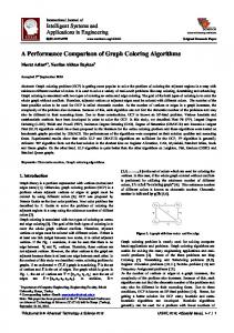
Fig. 1. Example showing how DOM colors a reducible graph

should be as close to minimum as possible. Here, we want to find out what is the role of Column Minimization in the overall success of a Decomposer; especially, in terms of the calculation time, the memory usage, and the quality of results. We want to investigate how the answers to these questions depend on the type of data, for instance on the percent of don’t cares, or on the density of graphs in question.

x.

There are basically four methods to find the Column Multiplicity in Functional Decomposition, namely Set Covering, Graph Coloring, Clique Partitioning and Clique Covering. A relation between the columns of the Karnaugh map of a function, for a given bound and free sets can be represented as a Compatibility Graph or as an Incompatibility Graph. If represented as a Compatibility Graph, nodes which are connected together are compatible nodes and can be colored with the same color. This is called Clique Covering. Even though there has been a lot of research done in the field of Graph Coloring and Functional Decomposition, nobody, to our knowledge, has compared these methods, or evaluated the importance of finding minimal solutions to the problem of Column Multiplicity in the Curtis Decomposition. There exist hundreds exact and heuristic graphcoloring and clique finding algorithms in the literature, to mention just [ I , 2 , 3, 4, 5 , 9, I I , 12, 13, 14, 17, 201 and in the past we programmed and compared several of them [8,21,22,23,25]. Although we are not able to study all published papers, we did not find an algorithm similar to our algorithm DOM), which is very fast, and gives good results. It uses domination coverings to color the graph and makes use of the fact that many graphs are colored with known values of p(,/)*. (The names domination and covering are used here with different meanings than in Graph Theory). In result, we obtain very high quality decompositions quite quickly, which positions our decomposer on top for nearly all tested by us benchark functions, not only from ISCAS and MCNC benchmarks, but also for KDD, Data Mining and ML benchmarks from U.C. Irvine and Wright Labs that have very high percent of don’t cares. (Moreover, our method is for multi-output decompositions, which allows to use it also for FSMs [7, 19, 161).

that is close to x. Because two-level decomposition stage is repeated very many times on all second, third, etc. levels, the stages of graph creation and graph coloring in S T E P 2 must be thoroughly designed. They are very important to the overall success of a Functional Decomposer program, because a high percentage of the run time of the Functional Decomposer is spent on the Column Minimization part of Decomposition [22,23]. One needs thus: (1) to create the graph quickly [6], (2) to color the graph quickly, but also the result

226

@ Removenode 1 * /

@ ‘

+- P A o . 7 and 5 bseudo-

Q

0

0

0

covering

(4

(‘1)

(C)

Fig. 2. Example showing how DOM colors a non-reducible graph

2. A New Algorithm DOM for Graph Coloring based on Domination Covering

that only few non-reducible graphs are created by DOM, this class is well-colorable by DOM. The number of removals is the upper bound on the difference p - x. The following explains how DOM colors a reducible graph. [l.] Fig. l(a) shows an Incompatibility Graph. Nodes 2 and 7 are covered by node 1, so in Fig. I(b) nodes 2 and 7 are removed and it is remembered that they were covered by node 1. [2.] Next, in Fig. l(b) node 5 is removed as it is covered by node 4, and it is remembered that node 4 covers node 5. 13.1 After removing node 7 the resulting graph shown in Fig. l(d).is a complete graph. [4.] In Fig. I(e), each node in the Complete Graph is given a unique color. [S.] In Fig. 1(t) the covered nodes are colored with the same color as the covering node. The color assignments are: Color A { I , 2, 7}, Color B {3}, Color C (4, 5 } , Color D 1 6 }. Fig. l(e) shows the completely colored graph. Four colors were used which is the minimum required for this graph. (p = exact solution was found). Example showing how DOM colors a non-reducible graph. [l.] An incompatibility graph is shown in Fig. 2(a), This graph is not reducible. 12.1 As the first step the graph is checked for coverings, but no coverings are found in this graph, so the first node (random) is removed from the graph, which is node 1, and it is assigned a minimum possible color which in this case is color A. [3.] This results in a new graph, shown in Fig. 2(b). In this graph node 4 covers node 2 and node 6. So node 2 and node 6 are removed from the graph, and it is remembered that node 4 covers node 2 and node 6. [4.] On removing node 2 and node 6, in the resulting graph shown in Fig. 2(c) nodes 3 and 5 have a pseudo-covering so the first one of these nodes which is node 3 is removed, and then node 4,5, and 7 form a complete graph. The complete graph is shown in Fig. 2(d). [5.] Now nodes are colored with the minimum possible color, and each covered node is given the same color as the node which covered it. The coloring is shown in Fig. 2(e). Three colors were used to color the graph, which is the minimum required for this graph. The color assignments are: Color A { 1, 3, 5 } , Color B {7}, Color C {2,4,6}. In the example like this no proof of exact solution can be given but only few consecutive graphs (here, only the initial graph) were non-reducible; so the solution is of a good quality (here, p differs by not more than one color from x). We showed experimentally elsewhere that DOM departs from the exact minimum for large random graphs, but we will demonstrate experimentally here that it will perform well in most cases on real-life benchmarks from decomposition. One weak point of the algorithm is when no coverings or pseudo-coverings are found at any stage of the coloring, then a node is selected and assigned a minimum possible color. If the coloring of this node is a bad choice, it will result in a solution which is not minimal. But experiments show that such complicated graphs(worst case graphs) will rarely, if ever, occur during the Column Minimization steps of decomposition, which is our application. When is equal or slightly higher than the size of the maximum clique, which is the case in our graphs, the results are very good. The strong point of DOM is that it can find the minimum solution without backtracking in all cases when the graph which results after checking for coverings is a complete graph. Thus this program will be effective in finding the minimum solution in all reducible graphs. Observe that if, for instance, p = 7 is found and the x = 6, then still only 3 wires (2’ > 7) are needed for output of block G , so the only loss of non-exact coloring is one column of

x.

Definition 1 A node “A” in an incompatibility graph covers some other node “B” in the graph if all of the following are satisfied: 1 ) Node “A” and node “B” have no common edge. 2 ) Node “A” has edges with all the nodes that node “B” has edges with. 3 ) Node “A” has at least one more edge than node “B”. When two nodes have a covering then both the nodes can be colored with the same color.

Definition 2 I f conditions I) and 2 )for coverings are satisfied and node “A” has the same number of edges as node “B”, then it is called a pseudo-covering. Theorem 1 Ifany node “ A ” in a graph coversany other node “B” in the graph, node “B” can be removed from the graph, and in a pseudo-covering any one of the nodes “A” or “B” can be removed. Definition 3 A Complete graph is one in which all pairs of vertices are connected. In a complete graph, total-edges = 2 , where total-edges is the sum of all the edges in the graph. In a Complete Graph no coverings or pseudo-coverings can be found and all nodes must have unique colors. Fig. Id shows a complete graph with 4 nodes. Definition 4 A non-reducible graph is a graph that is not complete and has no coveredor pseudo-coveredrtode(s). Graphs from Fig. la,b,c are reducible. The graph from Fig. 2a is non-reducible. Graphs from Fig. 2b,c are reducible, and graph from Fig. 2d is complete. Theorem 2 I f a graph is reducible and can be reduced to a complete graph by successive removing of all its covered andpseudocovered nodes, then Algorithm DOM finds the coloring with the minimum number of colors (the exact coloring). Our approach to the Column Minimization Problem in Functional Decomposition is the following: For an arbitrary graph, it is assumed that the graph is reducible and the DOM algorithm is used. If it finds a solution by subsequent reduction and arrives at a complete graph without generating a non-reducible graph, we know that this solution is exact. If a non-reducible graph is generated, we color and remove a randomly selected node. The removal makes the graph reducible - in such case we have no proof of optimality, but still a good coloring is found if only few non-reducible graphs were consecutively converted to reducible graphs by the removal of nodes. Thus, if the characteristics of graphs of some class is

x

227

tical function benchmarks. We instantiated three algorithms into MVGUD, a Greedy Clique Partitioning (CLIP), the Dominance Graph Coloring ( D O N and the Exact Graph Coloring(EX0C). The decomposer was run with different numbers of variables in the Bound Set on two kinds of benchmarks: MCNC benchmarks for circuits (presented below), and ML Benchmarks (from the Wright Labs Database) for data from ML, Pattern Recognition and Knowledge Discovery in Data Bases. A comparison of DOM and EXOC was first done on randomly generated graphs, for varying number of nodes and varying percentage of edges (not shown because of a lack of space). Conclusions were reached about how well DOM and EXOC will perform on the different kinds of graphs. Tests were done to characterize the kind of graphs that are generated in decomposition with regard to the number of nodes in the graph and the percentage of edges in the graph in order to see if the same conclusions hold for the graphs generated during Functional Decomposition F = H ( G ( B ) , A ) . Whether the method used by MVGUD to calculate D F C is a good evaluation of the cost of the decomposed multi-valued blocks is not discussed here, but since the D F C is used for a comparison between different methods of calculating the Column Multiplicity in Decomposition, within the same decomposer, the method of calculation of the D F C does not matter for the purpose of evaluating algorithms for calculating column multiplicity. What matters is that the same method is used for all the algorithms that are compared. The goal of the testing is to see if an Exact Graph Coloring is necessary to calculate the Column Multiplicity in Functional Decomposition, and if the D F C can be improved in case that MVGUD is run with EXOC, in comparison to when it is run with DOM or with CLIP. MVGUD was tested with 2 - 5, and more variables in the Bound set (only some results are reported here because of space). Notations Used in the Tables. The following is an explanation of the Notations used in the Tables in this section: Bnch : Name of the Benchmark function; i: Number of inputs of the Benchmark: 0 : Number of outputs of the Benchmark; c: Number of cubes in the Benchmark; C: Decomposed function cardinality of the decomposed function; AI: Name of Algorithm used in MVGUD (E=EXOC, D=DOM, C=CLIPS); n bl: Number of multi-valued blocks in the decomposed function; NP: Number ofpasses,or number of times the function to calculate the column multiplicity was called; TC: Total Colors, iterative sum of colors generated for each pass; AC: Average Colors = TC/NP; T(s): User time in seconds. A comparison was first made by runningMVGUD with 2 variables in the Bound Set for EXOC, DOM and CLIP. Comparisons were made with respect to the DFC, the number of two-input gates in the final decomposed function, and the time taken by MVGUD to decompose the function. DOM provides a smaller DFC in 6 cases and CLIP provides a smaller DFC in 5 cases, while EXOC provides a tie with the best solution in 6 ofthe cases. Hence EXOCdoes not provide any real improvement, on the other hand it is much slower than CLIP and DOM, which is to be expected. The reason for this kind of results is that since in this experiment there are 2 variables in the Bound Set, in most cases the size of the Incompatibility Graph at different levels of the decomposition is 4, which is a small graph, and it is known that for small graphs both CLIP and DOM usually generate the best solution as well. Hence we conclude that for two variables in the Bound Set it is not worthwhile having an Exact Graph Coloring to calculate the Column Multiplicity in MVGUD,

A Comparison of results obtained by running MVGUD with 4 variables in the Bound Set on MCNC Benchmarks

A Comparison of Total Colors generated by DOM, and CLIP compared with total colors generated by EXOC on the same graphs for two, four and five variables in the Bound Set for ML Benchmarks

don't cares, instead of two columns of don't cares in case of exact coloring with p = Let us make a point that in both cases the number of new wires (functions) created is the minimum and the same (here, 3).

x.

3. An Evaluation of DOM on the Column Multiplicity Problem In this section we will evaluate the importance of an Exact Graph Coloring in Curtis Decompositions. Our aim is to investigate if an Exact Graph Coloring is required in Functional Decomposition and if it leads to better results on the graphs that are created from prac-

A Summary showing the Addition of the Total Colors obtained in Table 2

228

CI'I

and a good heuristic algorithm to calculate the Column Multiplicity is sufficient. Table 1 shows the result for 4 variables in the Bound Set. AV E% was calculated to see how dense or sparse the graphs generated during the decomposition are. This was calculated in the following way: For any graph with number of nodes = n , the total-possible-edges for this graph( 100% edges ) will be equal to n * ( n - l)/2. Hence if the number of edges in the graph is equal This to e, then the edgepercent = ( e * lOO)/totalpossible~dges. will give the edgegercent in a graph with n nodes and e edges. Since the decomposer calls the function to calculate the Column Multiplicity a number oftimes, the Av E% was calculated by adding the edgepercent for a graph each time the function to find Column Multiplicity was called, and then dividing this total by the number of times the function to calculate the Column Multiplicity was called. EXOC(E), DOM(D) and CLIP (C) generate the same results in all the cases in terms of DFC and number of CLB's. The reason for the slow times of MVGUD with EXOC can be explained as follows: when MVGUD is run with 5 variables (not shown) in the Bound set, in most cases the average number of nodes in the graph is 32 and the edge percentage is always high with the highest being 77% and the lowest being 46.1 % This means that the graphs generated during decomposition were nearly always (since this is an average) dense graphs. It was found experimentally on random graphs that for dense graphs EXOC takes a long time to find the Exact solution, hence we have such slow times for EXOC. Whenever DOM does not generate an exact solution, it is usually 1 or 2 colors away from the Exact solution and rarely more than that, and this being on randomly generated graphs. Now considering that there were 5 variables in the Bound Set, then the Incompatibility graph will have 32 nodes, and for a Curtis decomposition to exist, if a coloring of the graph with 16 colors or less is found then one exists. In a Table for 5 variables in the column for Average colors A C we would find that the largest average color is 7.65 for the benchmark sao2. But this means that these graphs generated during decomposition, had low chromatic numbers, which were much less than 16. So even if DOM or CLIP generate a solution that is 2 or 3 colors away, the solution will be accepted as a Curtis Decomposition because it will still be less than 16. The same reasoning applies to Table 1 where a comparison is made with 4 variables in the Bound Set. Hence we conclude that for 4 or 5 or greater number of variables in the Bound Set an Exact Graph Coloring does not produce better Curtis Decompositions, and having a good heuristic algorithm to find the Column Multiplicity or even a greedy algorithm to find the Column Multiplicity is good enough. By the results of the testing we can definitely say that we have proved that an Exact Graph Coloring is not required to find the Column Multiplicity where Curtis Decompositions are considered. Exact Graph Colorings only take up more time and fails to produce any significant change in the results. This is true with respect to both Circuit Benchmarks and ML Benchmarks (not presented here). Also the results shown raise the question that in cases where CLIP did not generate the same total numbers of colors as EXOC, why did the DFC not improve when we used EXOC? The only possible answer to this question is that the decompositions generated by CLIP were still acceptabledecompositions, even if they use non minimum numbers of colors which in turn means that these graphs generated during the decomposition process must be having low chromatic numbers. This provides a very valuable insight

FLIC SXpI 'J)

ZXX(9) IMYS)

YX4 OX

2428 37211 3'J2

a

ZSZ 672 SI6

4hX

464 42lM

m

J, 321yZll)

Jb 33921)

MI &34%(lIlU,

240 224 416 3112X 84 2.56 120

"x

2240)

2Sh(X) 2SNX) 352(11) 3lWIY) 76U(24)

MV

11.11 26.4

112XY.ll

z w

zi1n.o

22Y 3Y2

I0.I X.6 II~.II

rn MI

IMy.5) 2S9X) 576(18)

IMyS) 224(7) 576(1X) SIZ(16) 73fd46)

111so(33)im(si 41913)

a W 752(47)

i n s m i i n 4 1 x z ~14, i

2.3

70 2xm

Ul

ZXX(IH)

[iimrl

-4

13160 1.8 13.1 32.6 47.2 WI.lI

Y5S

1326

467

53

SI2(16) l8sYll6 IHW(114

lab e 4

into the kinds of graphs that are generated during the decomposition process: the graphs generated during the decomposition process are definitely of a different nature than random graphs. This is because it is known [24] that 98% of real-life functions is decomposable; thus their graphs have small (in contrast, only l% of randomly generated functions are decomposable). The result that random graphs are much more difficult than graphs originating from real-life problem is known from other EDA areas [9], but was not known for functional decomposition. As found in experiments EXOC was unable to provide a better DFC for the ML Benchmarks. In order to see the total numbers of colors generated by DOM, EXOC and CLIP on the same graphs, which were generated during the process of Functional Decomposition, the following experiment was performed: MVGUD was made to run with all three algorithms EXOC, CLIP, and DOM calculating the Column Multiplicity, and only the results of one of them was accepted and the results from the other two was discarded. The count of the colors was kept for all three Algorithms, thus demonstrating how EXOC, CLIP, and DOM compare with respect to the total number of colors generated on the same graphs, only now these graphs have been generated from practical function Benchmarks. Table 2 is a summary of the results of 46 program runs. It shows how DOM and CLIP compare with respect to the number of times that the total number of colors generated by DOM and CLIP are the same as the total number of colors generated by EXOC, and the number of times the total colors generated by DOM and CLIP were not exact and by how much. [l.] In Table 2, the row Exact stands for the case when the total numbers of colors generated by DOM and CLIP was the same as the total colors generated by EXOC. Error I stands for the case in which the total numbers of colors generated by DOM and CLIP were one color away from the total numbers of colors generated by EXOC, and so on, till Error6. Corresponding to these rows, the column Nu gives the number of times, and column % is equal to Nu/TotalNurnbero fProgramRuns* 100. [2.] As can be seen from the Table 2 , DOM performs extremely well, and CLIP does not perform so well. DOM thus proves to be a very good heuristic algorithm. [3.] Table 3 is a total of the rows of Table 2 for DOM and CLIP.

x

4. General Comparison of MVGUD with other Decomposers and Conclusions Table 4 shows the result of comparison of MVGUD and other decomposers on some benchmarks (recall that in contrast to others, we do not have a fixed number of inputs to a block). Observe that

229

REFERENCES

DFC allows to compare (only approximately) decomposers that decompose to various types and sizes of blocks. In Table, all the functions in the table are binary and are taken from the set of MCNC benchmarks. St is the binary decomposer from Freiberg (Steinbach). TRADE (MI) is an earlier decomposer developed at Portland State University [25]; MIS11 (MI) at University of California, Berkeley; SC is the Mulop-dc decomposer from Freiburg (Scholl) Js and Js are from Technical Univ. of Eindhoven (Jozwiak) (Js is systematic and Jh heuristic strategy); and LU is the Dernain program from Warsaw/Monash (Luba and Selvaraj) The final cost value is computed as a sum of the costs of DFCs of single blocks of the result of the decomposition. For MVGUD (MV) there is also execution time given (DECstation 5000/240,64 MB of memory, user time in seconds) to show that the decomposition task can be performed in a reasonable amount of time. Numbers in parentheses are numbers of 5-input CLBs (Jozwiak reports only 4-input CLBs). The underlined results are the best DFC values for a given benchmark. Our version of clip is different ( 9 3 , and we cannot find some of the benchmarks used by other authors.

[ I ] A.V. Anisirnov, “Local Optimization of Colorings of Graphs,” Cybernetics, Vol. 22, No. 6, pp. 683-692, 1986. [2] L. Babel. “Finding Maximum Cliques in Arbitrary and in Special

Graphs,” Contp. Vol46, pp. 321-341. 1991. [3] E.A. Bender, and H.S. Wilf, “A Theoretical Analysis of Backtracking in the Graph Coloring Problem,” pp. 275-282.J. (f’Alg., Vol. 6.

[41 A. Blurn. “New approximation algorithms for graph coloring:’JACM, Vol. 41, NO.3,pp. 470-516, 1994. [SI P. Briggs, K. Cooper. K. Kennedy, and L. Torczon, “Coloring Heuristics for Register Allocation,” ASCM Conf:on Progr: k i n . Des. Impl, pp. 275-284, ACM. 1989. [6] M. Burns. M. Perkowski. L. Jozwiak. “An Efficient Approach to Decomposition of Multi-Output Boolean Functions with Large Sets of Bound Variables,” Proc. 1998 Euromicro. pp. 16-23. Vasteras. Sweden, August 25-27, 1998. 171 A.N. Chehotarev, “Approach to Functional Specification of Automata,” Kibernetiku i Sisremnyj Anuliz, No. 3, pp. 31-42, 1991 (in Russian). [8] M.J. Ciesielski. S. Yang, and M.A. Perkowski, “Multiple-Valued Minimization Based on Graph Coloring,” . Proc. of ICCD’89, pp. 262 - 265. Oct. 1989. [9] 0. Coudert, “Coloring of Real-Life Graphs is Easy,” Pmc. DAC’97, 1997. [IO] H.A. Curtis, “A New Approach to the Design of Switching Circuits,” k n Nostrund, Princeton, N.J., 1962. [I I ] R. Diestel. “Graph Theory,”Springer, 1997. [ 121 E. C. Freuder, “A Sufficient Condition of Backtrack-Free Search,” JACM. Vol. 29, NO. I . pp. 24-32, 1982 [I31 M.R. Carey, and D.S. Johnson. “The Complexity of Near-Optimal Graph Coloring,” JACM. Vol. 23, No. I , Jan. 1976, pp. 43-49. [ 141 I.M. Gessel. “A coloring problem,” The Am. Muth. Monthly, Vol. 98, pp. 530-538, 1991. [ 151 S.Grygiel, M. Perkowski, M. Marek-Sadowska, T. Luba, L. Jozwiak. “Cube Diagram Bundles: A New Representation of Strongly Unspecified Multiple-Valued Functions and Relations,” froc. ISMVL’97. pp. 287-292. [I61 S. Grygiel, M. Perkowski, “New Compact Representation of Multiple-Valued Functions, Relations, and Non-Deterministic State Machines, Proc. ICCD’98. Oct. 5 , 1998. [I71 T.R. Jensen, and B. Toft,“Graph Coloring Problems,” Wiley, 1995. [IS] T.Luba, M. Mochocki, J. Rybnik, “Decomposition of Information Systems Using Decision Tables,” Bull. fd. Acud. Sei.. Techn. Sei., Vol. 41, No. 3, 1993. [ 191 A.A. Mishchenko. “A CAD System for Automated Synthesis of Controlling Automata,” Cyberrietics utrd System Anulysis, Plenum Press, NO. 3. pp. 23-30. 1997. [ZO] C. Morgenstern. “Improved Implementations of Dynamic Sequential Coloring Algorithms,” Dept. Comp. Sci, Texas Christ. Univ, 1991. [21] L. Nguyen. M. Perkowski, and N. Goldstein, “PALMINI - Fast Boolean Minimizer for Personal Computers,” Proc. ofDAC, pp. 615621,1987. [22] M.A. Perkowski, “A New Representation of Strongly Unspecified Switching Functions and it Application to Multi-Level AND/OR/EXOR Synthesis.”Proc. RM’9.5Work, 1995. pp. 143-151. [23] M. Perkowski, M. Marek-Sadowska, L. Jozwiak, M. Nowicka, R. Malvi, Z. Wang, J. Zhang, “Decomposition of Multiple-Valued Relations,” Proc. ISMVL’97,pp. 13-18. [24] T.D. Ross, M.J. Noviskey, T.N. Taylor, D.A. Gadd, “Pattern Theory: An Engineering Paradigm for Algorithm Design,” Final Technical Report WL-TR-9 1 - 1060, Wright Laboratories, USAF, WUAARTNPAFB. OH 45433-6543. August 199I. [ Z S ] W. Wan. M.A. Perkowski, “A New Approach to the Decomposition of Incompletely Specified Multi-Output Functions Based on GraphColoring and Local Transformations and its Application to FPGA mapping,’’Pmc. (#EURO-DAC’92, pp. 230-235, 1992.

Concluding, in order to create an efficient and effective program for the Column Multiplicity in Curtis decomposition, it was necessary to analyse its stages systematically. Our achievements are:

1 The new algorithm for incompatibility graph creation, GCA, is always faster, and for larger bound sets it is orders of magnitude faster than the previous algorithm PCA used in other decomposers, producing the same graphs [6]. 2 The new heuristic Dominance Coloring program, DOM was compared with heuristic Clique Partitioning CLIP used in previous research. It was shown that DOM performs better, because it gives exact solutions on some types of graphs, which happen to be quite common in decomposition. 3 DOM was compared with the Exact Graph Coloring algorithm EXOC. It was shown that Exact Algorithm is not needed to find the minimum Column Multiplicity for Curtis Decompositions on graphs from decomposition, because it is much slower on larger bound sets and gives the same or only slightly better results. In many various type experiments we clearly demonstrated that the incompatibility graphs generated during the decomposition process are much simpler than graphs generated randomly (for which Exact algorithm gives much better results, as may be expected for NPcomplete problem).

4 The DOM graph reduction can be seen as a preprocessing step, so it could be applied to any other heuristic or exact graph coloring algorithm.

5 The introduction of the idea of fast early filtering of decompositions by using clique size and H,,,,, values for the cut-oft’ of the graph creation process, of the further graph coloring process, and of the G and H calculation processes. 6 Because using GCA and DOM together we can create and color graphs quickly, we can test many more bound set candidates, and also larger bound sets, in the same time. Thus, our decomposer can find relatively quickly hierarchical decompositions of smaller complexity. DFC of our solutions is in most cases smaller than that for other decomposers. Thus, we created a highly efficient and effective decomposer, and, paraphrasing 0. Coudert, [9] we showed experimentally that “Column Minimization for Curtis Decomposition is Easy.”

230