Graph Embedding Techniques, Applications, and Performance - arXiv

IEEE TRANSACTIONS ON PATTERN ANALYSIS AND MACHINE INTELLIGENCE, VOL. XX, NO. XX, MAY 2017

1

Graph Embedding Techniques, Applications, and Performance: A Survey

arXiv:1705.02801v2 [cs.SI] 9 May 2017

Palash Goyal and Emilio Ferrara Abstract—Graphs, such as social networks, word co-occurrence networks, and communication networks, occur naturally in various real-world applications. Analyzing them yields insight into the structure of society, language, and different patterns of communication. Many approaches have been proposed to perform the analysis. Recently, methods which use the representation of graph nodes in vector space have gained traction from the research community. In this survey, we provide a comprehensive and structured analysis of various graph embedding techniques proposed in the literature. We first introduce the embedding task and its challenges such as scalability, choice of dimensionality, and features to be preserved, and their possible solutions. We then present three categories of approaches based on factorization methods, random walks, and deep learning, with examples of representative algorithms in each category and analysis of their performance on various tasks. We evaluate these state-of-the-art methods on a few common datasets and compare their performance against one another and versus non-embedding based models. Our analysis concludes by suggesting some potential applications and future directions. We finally present the open-source Python library, named GEM (Graph Embedding Methods), we developed that provides all presented algorithms within a unified interface, to foster and facilitate research on the topic. Index Terms—Graph embedding techniques, Graph embedding applications, Python Graph Embedding Methods GEM Library

F

1

I NTRODUCTION

G

RAPH analysis has been attracting increasing attention in the recent years due the ubiquity of networks in the real world. Graphs (a.k.a. networks) have been used to denote information in various areas including biology (Protein-Protein interaction networks) [1], social sciences (friendship networks) [2] and linguistics (word co-occurrence networks) [3]. Modeling the interactions between entities as graphs has enabled researchers to understand the various network systems in a systematic manner [4]. For example, social networks have been used for applications like friendship or content recommendation, as well as for advertisement [5]. Graph analytic tasks can be broadly abstracted into the following four categories: (a) node classification [6], (b) link prediction [5], (c) clustering [7], and (d) visualization [8]. Node classification aims at determining the label of nodes (a.k.a. vertices) based on other labeled nodes and the topology of the network. Link prediction refers to the task of predicting missing links or links that are likely to occur in the future. Clustering is used to find subsets of similar nodes and group them together; finally, visualization helps in providing insights into the structure of the network. In the past few decades, many methods have been proposed for the tasks defined above. For node classification, there are broadly two categories of approaches — methods which use random walks to propagate the labels [9], [10], and methods which extract features from nodes and apply classifiers on them [11], [12]. Approaches for link prediction include similarity based methods [13], [14], maximum likelihood models [15], [16], and probabilistic models [17],

•

Palash Goyal and Emilio Ferrara are with the Department of Computer Science, University of Southern California (USC), and with the USC Information Sciences Institute.

Manuscript received April 24, 2017.

[18]. Clustering methods include attribute based models [19] and methods which directly maximize (resp., minimize) the inter-cluster (resp., intra-cluster) distances [7], [20]. This survey will provide a taxonomy that captures these application domains and the existing strategies. Typically, a model defined to solve graph-based problems either operates on the original graph adjacency matrix or on a derived vector space. Recently, the methods based on representing networks in vector space, while preserving their properties, have become widely popular [21], [22], [23]. Obtaining such an embedding is useful in the tasks defined above.1 The embeddings are input as features to a model and the parameters are learned based on the training data. This obviates the need for complex classification models which are applied directly on the graph. 1.1

Challenges

Obtaining a vector representation of each node of a graph is inherently difficult and poses several challenges which have been driving research in this field: (i) Choice of property: A “good” vector representation of nodes should preserve the structure of the graph and the connection between individual nodes. The first challenge is choosing the property of the graph which the embedding should preserve. Given the plethora of distance metrics and properties defined for graphs, this choice can be difficult and the performance may depend on the application. (ii) Scalability: Most real networks are large and contain millions of nodes and edges — embedding methods should 1. The term graph embedding has been used in the literature in two ways: to represent an entire graph in vector space, or to represent each individual node in vector space. In this paper, we use the latter definition since such representations can be used for tasks like node classification, differently from the former representation.

IEEE TRANSACTIONS ON PATTERN ANALYSIS AND MACHINE INTELLIGENCE, VOL. XX, NO. XX, MAY 2017

be scalable and able to process large graphs. Defining a scalable model can be challenging especially when the model is aimed to preserve global properties of the network. (iii) Dimensionality of the embedding: Finding the optimal dimensions of the representation can be hard. For example, higher number of dimensions may increase the reconstruction precision but will have high time and space complexity. The choice can also be application-specific depending on the approach: E.g., lower number of dimensions may result in better link prediction accuracy if the chosen model only captures local connections between nodes. 1.2

Our contribution

This survey provides a three-pronged contribution: (1) We propose a taxonomy of approaches to graph embedding, and explain their differences. We define four different tasks, i.e., application domains of graph embedding techniques. We illustrate the evolution of the topic, the challenges it faces, and future possible research directions. (2) We provide a detailed and systematic analysis of various graph embedding models and discuss their performance on the various tasks. For each method, we analyze the properties preserved and its accuracy, through comprehensive comparative evaluation on a few common data sets and application scenarios. (3) To foster further research in this topic, we finally present GEM, the open-source Python library we developed that provides, under a unified interface, implementations of all graph embedding methods discussed in this survey. To the best of our knowledge, this is the first paper to survey graph embedding techniques and their applications. 1.3

Organization of the survey

The survey is organized as follows. In Section 2, we provide the definitions required to understand the problem and models discussed next. Section 3 proposes a taxonomy of graph embedding approaches and provides a description of representative algorithms in each category. The list of applications for which researchers have used the representation learning approach for graphs is provided in Section 4. We then describe our experimental setup (Section 5) and evaluate the different models (Section 6). Section 7 introduces our Python library for graph embedding methods. Finally, in Section 8 we draw our conclusions and discuss potential applications and future research direction.

2

2

Definition 2. (First-order proximity) Edge weights sij are also called first-order proximities between nodes vi and vj , since they are the first and foremost measures of similarity between two nodes. We can similarly define higher-order proximities between nodes. For instance, Definition 3. (Second-order proximity) The second-order proximity between a pair of nodes describes the proximity of the pair’s neighborhood structure. Let si = [si1 , · · · , sin ] denote the first-order proximity between vi and other nodes. Then, second-order proximity between vi and vj is determined by the similarity of si and sj . Second-order proximity compares the neighborhood of two nodes and treats them as similar if they have a similar neighborhood. It is possible to define higher-order proximities using other metrics, e.g. Katz Index, Rooted PageRank, Common Neighbors, Adamic Adar, etc. (for detailed definitions, omitted here in the interest of space, see Ou et al. [24]). Next, we define a graph embedding: Definition 4. (Graph embedding) Given a graph G = (V, E), a graph embedding is a mapping f : vi → yi ∈ Rd ∀i ∈ [n] such that d  |V | and the function f preserves some proximity measure defined on graph G. An embedding therefore maps each node to a lowdimensional feature vector and tries to preserve the connection strengths between vertices. For instance, an embedding preserving P first-order proximity might be obtained by minimizing i,j sij kyi − yj k22 . Let two node pairs (vi , vj ) and (vi , vk ) be associated with connections strengths such that sij > sik . In this case, vi and vj will be mapped to points in the embedding space that will be closer each other than the mapping of vi and vk .

3

A LGORITHMIC A PPROACHES : A TAXONOMY

In the past decade, there has been a lot of research in the field of graph embedding, with a focus on designing new embedding algorithms. More recently, researchers pushed forward scalable embedding algorithms that can be applied on graphs with millions of nodes and edges. In the following, we provide historical context about the research progress in this domain (§3.1), then propose a taxonomy of graph embedding techniques (§3.2) covering (i) factorization methods (§3.3), (ii) random walk techniques (§3.4), (iii) deep learning (§3.5), and (iv) other miscellaneous strategies (§3.6).

D EFINITIONS AND P RELIMINARIES

We represent the set {1, · · · , n} by [n] in the rest of the paper. We start by formally defining several preliminaries which have been defined similar to Wang et al. [23]. Definition 1. (Graph) A graph G(V, E) is a collection of V = {v1 , · · · , vn } vertices (a.k.a. nodes) and E = {eij }ni,j=1 edges. The adjacency matrix S of graph G contains nonnegative weights associated with each edge: sij ≥ 0. If vi and vj are not connected to each other, then sij = 0. For undirected weighted graphs, sij = sji ∀i, j ∈ [n]. The edge weight sij is generally treated as a measure of similarity between the nodes vi and vj . The higher the edge weight, the more similar the two nodes are expected to be.

3.1

Graph Embedding Research Context and Evolution

In the early 2000s, researchers developed graph embedding algorithms as part of dimensionality reduction techniques. They would construct a similarity graph for a set of n D-dimensional points based on neighborhood and then embed the nodes of the graph in a d-dimensional vector space, where d  D. The idea for embedding was to keep connected nodes closer to each other in the vector space. Laplacian Eigenmaps [25] and Locally Linear Embedding (LLE) [26] are examples of algorithms based on this rationale. However, scalability is a major issue in this approach, whose time complexity is O(|V |2 ).

IEEE TRANSACTIONS ON PATTERN ANALYSIS AND MACHINE INTELLIGENCE, VOL. XX, NO. XX, MAY 2017

Since 2010, research on graph embedding has shifted to obtaining scalable graph embedding techniques which leverage the sparsity of real-world networks. For example, Graph Factorization [21] uses an approximate factorization of the adjacency matrix as the embedding. LINE [22] extends this approach and attempts to preserve both first order and second proximities. HOPE [24] extends LINE to attempt preserve high-order proximity by decomposing the similarity matrix rather than adjacency matrix using a generalized Singular Value Decomposition (SVD). SDNE [23] uses autoencoders to embed graph nodes and capture highly nonlinear dependencies. The new scalable approaches have a time complexity of O(|E|).

3.2

A Taxonomy of Graph Embedding Methods

We propose a taxonomy of embedding approaches. We categorize the embedding methods into three broad categories: (1) Factorization based, (2) Random Walk based, and (3) Deep Learning based. Below we explain the characteristics of each of these categories and provide a summary of a few representative approaches for each category (cf. Table 1), using the notation presented in Table 2.

3.3

Factorization based Methods

Factorization based algorithms represent the connections between nodes in the form of a matrix and factorize this matrix to obtain the embedding. The matrices used to represent the connections include node adjacency matrix, Laplacian matrix, node transition probability matrix, and Katz similarity matrix, among others. Approaches to factorize the representative matrix vary based on the matrix properties. If the obtained matrix is positive semidefinite, e.g. the Laplacian matrix, one can use eigenvalue decomposition. For unstructured matrices, one can use gradient descent methods to obtain the embedding in linear time. 3.3.1

Locally Linear Embedding (LLE)

LLE [26] assumes that every node is a linear combination of its neighbors in the embedding space. If we assume that the adjacency matrix element Wij of graph G represents the weight of node j in the representation of node i, we define X Yi ≈ Wij Yj ∀i ∈ V. j

Hence, we can obtain the embedding Y N ×d by minimizing X X φ(Y ) = |Yi − Wij Yj |2 , i

3.3.2

3

Laplacian Eigenmaps

Laplacian Eigenmaps [25] aim to keep the embedding of two nodes close when the weight Wij is high. Specifically, they minimize the following objective function

φ(Y ) =

1X (Yi − Yj )2 Wij 2 i,j

= Y T LY, where L is the Laplacian of graph G. The solution to this can be obtained by taking the eigenvectors corresponding to the d smallest eigenvalues of the normalized Laplacian, Lnorm = D−1/2 LD−1/2 . 3.3.3

Graph Factorization (GF)

To the best of our knowledge, Graph Factorization [21] was the first method to obtain a graph embedding in O(|E|) time. To obtain the embedding, GF factorizes the adjacency matrix of the graph, minimizing the following loss function

φ(Y, λ) =

1 X λX kYi k2 , (Wij − < Yi , Yj >)2 + 2 2 i (i,j)∈E

where λ is a regularization coefficient. Note that the summation is over the observed edges as opposed to all possible edges. This is an approximation in the interest of scalability, and as such it may introduce noise in the solution. Note that as the adjacency matrix is often not positive semidefinite, the minimum of the loss function is greater than 0 even if the dimensionality of embedding is |V |. 3.3.4

GraRep

GraRep [27] defines the node transition probability as T = D−1 W and preserves k -order proximity by minimizing kX k − Ysk YtkT k2F where X k is derived from T k (refer to [27] for a detailed derivation). It then concatenates Ysk for all k to form Ys . Note that this is similar to HOPE [24] which minimizes kS − Ys YtT k2F where S is an appropriate similarity matrix. The drawback of GraRep is scalability, since T k can have O(|V |2 ) non-zero entries. 3.3.5

HOPE

HOPE [24] preserves higher order proximity by minimizing kS − Ys YtT k2F , where S is the similarity matrix. The authors experimented with different similarity measures, including Katz Index, Rooted Page Rank, Common Neighbors, and Adamic-Adar score. They represented each similarity measure as S = Mg−1 Ml , where both Mg and Ml are sparse. This enables HOPE to use generalized Singular Value Decomposition (SVD) [30] to obtain the embedding efficiently.

j

To remove degenerate solutions, the variance of the embed1 ding is constrained as N Y T Y = I . To further remove translational invariance, the embedding is centered around zero: P Y = 0. The above constrained optimization problem i i can be reduced to an eigenvalue problem, whose solution is to take the bottom d + 1 eigenvectors of the sparse matrix (I − W )T (I − W ) and discarding the eigenvector corresponding to the smallest eigenvalue.

3.4

Random Walk based Methods

Random walks have been used to approximate many properties in the graph including node centrality [31] and similarity [32]. They are especially useful when one can either only partially observe the graph, or the graph is too large to measure in its entirety. Embedding techniques using random walks on graphs to obtain node representations have been proposed: DeepWalk and node2vec are two examples.

IEEE TRANSACTIONS ON PATTERN ANALYSIS AND MACHINE INTELLIGENCE, VOL. XX, NO. XX, MAY 2017

4

TABLE 1 List of graph embedding approaches Category

Year

Published

Authors/Lab

Method

Time Complexity

Random Walk

2000 2001 2013 2015 2016 2014 2016

Science [26] NIPS [25] WWW [21] CIKM [27] KDD [24] KDD [28] KDD [29]

Roweis & Saul Belkin & Niyogi Google Research IBM Research P. Cui & al. S. Skienna & al. J. Leskovec & al.

LLE Laplacian Eigenmaps Graph Factorization GraRep HOPE DeepWalk node2vec

O(|E|d2 ) O(|E|d2 ) O(|E|d) O(|V |3 ) O(|E|d2 ) O(|V |) O(|V |)

Deep learning

2016

KDD [23]

P. Cui & al.

SDNE

O(|V ||E|)

1st and 2nd order proximities

Miscellaneous

2015

WWW [22]

Microsoft Research

LINE

O(|E|d)

1st and 2nd order proximities

Factorization

TABLE 2 Summary of notation G

Graphical representation of the data

V

Set of vertices in the graph

E

Set of edges in the graph

d

Number of dimensions

Y

Embedding of the graph, |V | × d

Yi

Embedding of node vi , 1 × d (also ith row of Y )

Ys

Source embedding of a directed graph, |V | × d

Yt

Target embedding of a directed graph, |V | × d

W

Adjacency matrix of the graph, |V | × |V |

D

Diagonal matrix of the degree of each vertex, |V | × |V |

L

Graph Laplacian (L = D − W ), |V | × |V |

< Y i , Yj >

Inner product of Yi and Yj i.e. Yi YjT

S

Similarity matrix of the graph, |V | × |V |

3.4.1

DeepWalk

DeepWalk [28] preserves higher-order proximity between nodes by maximizing the probability of observing the last k nodes and the next k nodes in the random walk centered at vi , i.e. maximizing log P r(vi−k , . . . , vi−1 , vi+1 , . . . , vi+k |Yi ), where 2k + 1 is the length of the random walk. 3.4.2

node2vec

Similar to DeepWalk [28], node2vec [29] preserves higherorder proximity between nodes by maximizing the probability of occurrence of subsequent nodes in fixed length random walks. The crucial difference from DeepWalk is that node2vec employs biased-random walks that provide a trade-off between breadth-first (BFS) and depth-first (DFS) graph searches, and hence produces higher-quality and more informative embeddings than DeepWalk. Choosing the right balance enables node2vec to preserve community structure as well as structural equivalence between nodes. 3.5

Deep Learning based Methods

The growing research on deep learning has led to a deluge of deep neural networks based methods applied to graphs [23], [33], [34]. Deep autoencoders have been e.g. used for dimensionality reduction [35] due to their ability to model non-linear structure in the data. Recently, SDNE [23] utilized this ability of deep autoencoder to generate an embedding model that can capture non-linearity in graphs.

Properties preserved 1st order proximity

1 − kth order proximities 1 − kth order proximities, structural equivalence

3.5.1 SDNE Wang et al. [23] proposed to use deep autoencoders to preserve the first and second order network proximities. They achieve this by jointly optimizing the two proximities. The approach uses highly non-linear functions to obtain the embedding. The model consists of two parts: unsupervised and supervised. The former consists of an autoencoder aiming at finding an embedding for a node which can reconstruct its neighborhood. The latter is based on Laplacian Eigenmaps [25] which apply a penalty when similar vertices are mapped far from each other in the embedding space. 3.6

Other Methods

3.6.1 LINE LINE [22] explicitly defines two functions, one each for firstand second-order proximities, and minimizes the combination of the two. The function for first-order proximity is similar to that of Graph Factorization (GF) [21] in that they both aim to keep the adjacency matrix and dot product of embeddings close. The difference is that GF does this by directly minimizing the difference of the two. Instead, LINE defines two joint probability distributions for each pair of vertices, one using adjancency matrix and the other using the embedding. Then, LINE minimizes the KullbackLeibler (KL) divergence of these two distributions. The two distributions and the objective function are as follows

1 1 + exp(− < Yi , Yj >) Wij pˆ1 (vi , vj ) = P (i,j)∈E Wij p1 (vi , vj ) =

O1 = KL(pˆ1 , p1 ) X O1 = − Wij log p1 (vi , vj ). (i,j)∈E

The authors similarly define probability distributions and objective function for the second-order proximity. 3.7

Discussion

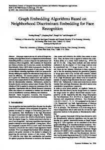
We can interpret embeddings as representations which describe graph data. Thus, embeddings can yield insights into the properties of a network. We illustrate this in Figure 1. Consider a complete bipartite graph G. An embedding algorithm which attempts to keep two connected nodes

IEEE TRANSACTIONS ON PATTERN ANALYSIS AND MACHINE INTELLIGENCE, VOL. XX, NO. XX, MAY 2017

1 2 3

5



6



7

 

8





 





       

(a) Graph G1

 



(b) CPE for G1











 











 





 



 







  



(c) SPE for G1





(d) Graph G2







4

5









 



(e) CPE for G2











(f) SPE for G2

Fig. 1. Examples illustrating the effect of type of similarity preserved. Here, CPE and SPE stand for Community Preserving Embedding and Structural-equivalence Preserving Embedding, respectively.

close (i.e., preserve the community structure), would fail to capture the structure of the graph — as shown in 1(b). However, an algorithm which embeds structurally-equivalent nodes together learns an interpretable embedding — as shown in 1(c). Similarly, in 1(d) we consider a graph with two star components connected through a hub. Nodes 1 and 3 are structurally equivalent (they link to the same nodes) and are clustered together in 1(f), whereas in 1(e) they are far apart. The classes of algorithms above can be described in terms of their ability to explain the properties of graphs. Factorization-based methods are not capable of learning an arbitrary function, e.g., to explain network connectivity. Thus, unless explicitly included in their objective function, they cannot learn structural equivalence. In random walk based methods, the mixture of equivalences can be controlled to a certain extent by varying the random walk parameters. Deep learning methods can model a wide range of functions following the universal approximation theorem [36]: given enough parameters, they can learn the mix of community and structural equivalence, to embed the nodes such that the reconstruction error is minimized. We can interpret the weights of the autoencoder as a representation of the structure of the graph. For example, 1(c) plots the embedding learned by SDNE for the complete bipartite graph G1 . The autoencoder stored the bipartite structure in weights and achieved perfect reconstruction. Given the variety of properties of real-world graphs, using general non-linear models that span a large class of functions is a promising direction that warrants further exploration.

4

A PPLICATIONS

As graph representations, embeddings can be used in a variety of tasks. These applications can be broadly classified as: network compression (§4.1), visualization (§4.2), clustering (§4.3), link prediction (§4.4), and node classification (§4.5).

4.1

Network Compression

Feder et al. [37] introduced the concept of network compression (a.k.a. graph simplification). For a graph G, they defined a compression G∗ which has smaller number of edges. The goal was to store the network more efficiently and run graph analysis algorithms faster. They obtained the compression graph by partitioning the original graph into bipartite cliques and replacing them by trees, thus reducing the number of edges. Over the years, many researchers have used aggregation based methods [38], [39], [40] to compress graphs. The main idea in this line of work is to exploit the link structure of the graph to group nodes and edges. Navlakha et al. [41] used Minimum Description Length (MDL) [42] from information theory to summarize a graph into a graph summary and edge correction. Similar to these representations, graph embedding can also be interpreted as a summarization of graph. Wang et al. [23] and Ou et al. [24] tested this hypothesis explicitly by reconstructing the original graph from the embedding and evaluating the reconstruction error. They show that a low dimensional representation for each node (in the order of 100s) suffices to reconstruct the graph with high precision. 4.2

Visualization

Application of visualizing graphs can be dated back to 1736 when Euler used it to solve ”Konigsberger Bruckenproblem” [43]. In the recent years, graph visualization has found applications in software engineering [44], electrical circuits [45], biology [1] and sociology [2]. Battista et al. [45] and Eades et al. [46] survey a range of methods used to draw graphs and define aesthetic criteria for this purpose. Herman et al. [47] generalize this and view it from an information visualization perspective. They study and compare various traditional layouts used to draw graphs including tree-, 3D- and hyperbolic-based layouts.

IEEE TRANSACTIONS ON PATTERN ANALYSIS AND MACHINE INTELLIGENCE, VOL. XX, NO. XX, MAY 2017

As embedding represents a graph in a vector space, dimensionality reduction techniques like Principal Component Analysis (PCA) [48] and t-distributed stochastic neighbor embedding (t-SNE) [8] can be applied on it to visualize the graph. The authors of DeepWalk [28] illustrated the goodness of their embedding approach by visualizing the Zachary’s Karate Club network. The authors of LINE [22] visualized the DBLP co-authorship network, and showed that LINE is able to cluster together authors in the same field. The authors of SDNE [23] applied it on 20-Newsgroup document similarity network to obtain clusters of documents based on topics. 4.3

Clustering

Graph clustering (a.k.a., network partitioning) can be of two types: (a) structure based, and (b) attribute based clustering. The former can be further divided into two categories, namely community based, and structurally equivalent clustering. Structure-based methods [7], [20], [49], aim to find dense subgraphs with high number of intra-cluster edges, and low number of inter-cluster edges. Structural equivalence clustering [50], on the contrary, is designed to identify nodes with similar roles (like bridges and outliers). Attribute based methods [19] utilize node labels, in addition to observed links, to cluster nodes. White et al. [51] used k -means on the embedding to cluster the nodes and visualize the clusters obtained on Wordnet and NCAA data sets verifying that the clusters obtained have intuitive interpretation. Recent methods on embedding haven’t explicitly evaluated their models on this task and thus it is a promising field of research in the graph embedding community. 4.4

Link Prediction

Networks are constructed from the observed interactions between entities, which may be incomplete or inaccurate. The challenge often lies in identifying spurious interactions and predicting missing information. Link prediction refers to the task of predicting either missing interactions or links that may appear in the future in an evolving network. Link prediction is pervasive in biological network analysis, where verifying the existence of links between nodes requires costly experimental tests. Limiting the experiments to links ordered by presence likelihood has been shown to be very cost effective. In social networks, link prediction is used to predict probable friendships, which can be used for recommendation and lead to a more satisfactory user experience. Liben-Nowell et al. [5], Lu et al. [52] and Hasan et al. [53] survey the recent progress in this field and categorize the algorithms into (a) similarity based (local and global) [13], [14], [54], (b) maximum likelihood based [15], [16] and (c) probabilistic methods [17], [18], [55]. Embeddings capture inherent dynamics of the network either explicitly or implicitly thus enabling application to link prediction. Wang et al. [23] and Ou et al. [24] predict links from the learned node representations on publicly available collaboration and social networks. In addition, Grover et al. [29] apply it to biology networks. They show that on these data sets links predicted using embeddings are more accurate than traditional similarity based link prediction methods described above.

4.5

6

Node Classification

Often in networks, a fraction of nodes are labeled. In social networks, labels may indicate interests, beliefs, or demographics. In language networks, a document may be labeled with topics or keywords, whereas the labels of entities in biology networks may be based on functionality. Due to various factors, labels may be unknown for large fractions of nodes. For example, in social networks many users do not provide their demographic information due to privacy concerns. Missing labels can be inferred using the labeled nodes and the links in the network. The task of predicting these missing labels is also known as node classification. Bhagat et al. [6] survey the methods used in the literature for this task. They classify the approaches into two categories, i.e., feature extraction based and random walk based. Feature-based models [11], [12], [56] generate features for nodes based on their neighborhood and local network statistics and then apply a classifier like Logistic Regression [57] and Naive Bayes [58] to predict the labels. Random walk based models [9], [10] propagate the labels with random walks. Embeddings can be interpreted as automatically extracted node features based on network structure and thus falls into the first category. Recent work [22], [23], [24], [28], [29] has evaluated the predictive power of embedding on various information networks including language, social, biology and collaboration graphs. They show that embeddings can predict missing labels with high precision.

5

E XPERIMENTAL S ETUP

Our experiments evaluate the feature representations obtained using the methods reviewed before on the previous four application domains. Next, we specify the datasets and evaluation metrics we used. The experiments were performed on a Ubuntu 14.04.4 LTS system with 32 cores, 128 GB RAM and a clock speed of 2.6 GHz. The GPU used for deep network based models was Nvidia Tesla K40C. 5.1

Datasets

We evaluate the embedding approaches on a synthetic and 6 real datasets. The datasets are summarized in Table 3. SYN-SBM: We generate synthetic graph using Stochastic Block Model [59] with 1024 nodes and 3 communities. We set the in-block and cross-block probabilities as 0.1 and 0.01 respectively. As we know the community structure in this graph, we use it to visualize the embeddings learnt by various approaches. KARATE [60]: Zachary’s karate network is a well-known social network of a university karate club. It has been widely studied in social network analysis. The network has 34 nodes, 78 edges and 2 communities. BLOGCATALOG [61]: This is a network of social relationships of the bloggers listed on the BlogCatalog website. The labels represent blogger interests inferred through the metadata provided by the bloggers. The network has 10,312 nodes, 333,983 edges and 39 different labels. YOUTUBE [62]: This is a social network of Youtube users. This is a large network containing 1,157,827 nodes and 4,945,382 edges. The labels represent groups of users who enjoy common video genres.

IEEE TRANSACTIONS ON PATTERN ANALYSIS AND MACHINE INTELLIGENCE, VOL. XX, NO. XX, MAY 2017

TABLE 3 Dataset Statistics Social Network

Synthetic

7

Collaboration Network

Biology Network

Name

SYN-SBM

KARATE

BLOGCATALOG

YOUTUBE

HEP-TH

ASTRO-PH

PPI

|V |

1024

34

10,312

1,157,827

7,980

18,772

3,890

|E|

29,833

78

333,983

4,945,382

21,036

396,160

38,739

Avg. degree

58.27

4.59

64.78

8.54

5.27

31.55

19.91

No. of labels

3

4

39

47

-

-

50

6

E XPERIMENTS AND A NALYSIS

HEP-TH [63]: The original dataset contains abstracts of papers in High Energy Physics Theory for the period from January 1993 to April 2003. We create a collaboration network for the papers published in this period. The network has 7,980 nodes and 21,036 edges. ASTRO-PH [64]: This is a collaboration network of authors of papers submitted to e-print arXiv during the period from January 1993 to April 2003. The network has 18,772 nodes and 396,160 edges. PROTEIN-PROTEIN INTERACTIONS (PPI) [65]: This is a network of biological interactions between proteins in humans. This network has 3,890 nodes and 38,739 edges.

In this section, we evaluate and compare embedding methods on the for tasks presented above. For each task, we show the effect of number of embedding dimensions on the performance and compare hyper parameter sensitivity of the methods. Furthermore, we correlate the performance of embedding techniques on various tasks varying hyper parameters to test the notion of an “all-good” embedding which can perform well on all tasks.

5.2

6.1

Evaluation Metrics

To evaluate the performance of embedding methods on graph reconstruction and link prediction, we use Precision at k (P r@k ) and M eanAverageP recision(M AP ) as our metrics. For node classification, we use micro-F1 and macroF1. These metrics are defined as follows: Pr@k is the fraction of correct predictions in top k |E (1:k)∩Eobs | predictions. It is defined as P r@k = pred k , where Epred (1 : k) are the top k predictions and Eobs are the observed edges. For the task of graph reconstruction, Eobs = E and for link prediction, Eobs is the set of hidden edges. MAP estimates precision for every node and computes the average over all nodes, as follows: P AP (i) , M AP = i |V | P

where AP (i) = |Epredi (1:k)∩Eobsi | , k

k

P r@k(i)·I{Epredi (k)∈Eobsi } , |{k:Epredi (k)∈Eobsi }|

P r@k(i) =

and Epredi and Eobsi are the predicted and observed edges for node i respectively. macro-F1, in a multi-label classification task, is defined as the average F 1 of all the labels, i.e., P F 1(l) , macro − F 1 = l∈L |L| where F 1(l) is the F 1-score for label l. micro-F1 calculates F 1 globally by counting the total true positives, false negatives and false positives, giving equal weight to each instance. It is defined as follows:

micro − F 1 = P

T P (l)

2∗P ∗R , P +R P

T P (l)

l∈L P , where P = P (Tl∈L P (l)+F P (l)) , and R = l∈L l∈L (T P (l)+F N (l)) are precision (P) and recall (R) respectively, and T P (l), F P (l) and F N (l) denote the number of true positives, false positives and false negatives respectively among the instances which are associated with the label l either in the ground truth or the predictions.

Graph Reconstruction

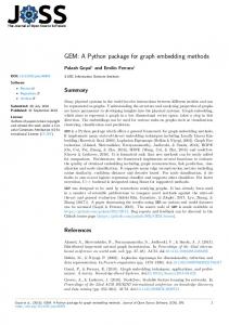
Embeddings as a low-dimensional representation of the graph are expected to accurately reconstruct the graph. Note that reconstruction differs for different embedding techniques (refer to Section 3). For each method, we reconstruct the proximity of nodes and rank pair of nodes according to their proximity. Then we calculate the ratio of real links in top k predictions as the reconstruction precision. As the number of possible node pairs (N (N − 1)) can be very large for networks with a large number of nodes, we randomly sample 1024 nodes for evaluation. We obtain 5 such samples for each dataset and calculate the mean and standard deviation of precision and MAP values for subgraph reconstruction. Figure 2 illustrates the reconstruction precision obtained by 128-dimensional embeddings. We observe that although performance of methods is dataset dependent, embedding approaches which preserve higher order proximities in general outperform others. Exceptional performance of Laplacian Eigenmaps on SBM can be attributed to the lack of higher order structure in the data set. We also observe that SDNE reconstruction with decoder outperforms other methods whereas Euclidean reconstruction is unable to achieve high precision. Similarly, embeddings learnt by node2vec have low reconstruction precision. This may be due to the highly non-linear dimensionality reduction yielding a nonlinear manifold. However, HOPE, which learns linear embeddings but preserves higher order proximity reconstructs the graph well without any additional parameters. Effect of dimension. Figure 3 illustrates the effect of dimension on the reconstruction error. With a couple of exceptions, as the number of dimensions increase, the MAP value increases. This is intuitive as higher number of dimensions are capable of storing more information. We also observe that SDNE is able to embed the graphs in 16dimensional vector space with high precision although decoder parameters are required to obtain such precision.

IEEE TRANSACTIONS ON PATTERN ANALYSIS AND MACHINE INTELLIGENCE, VOL. XX, NO. XX, MAY 2017

1.0

1.0

0.9 0.7 0.6

Method

0.5 0.4 0.3 0.2 0 2

LE GF n2v SDNE HOPE

0.8

Method

LE GF n2v SDNE HOPE

0.6 0.4 0.2

24

22

k

26

28

0.0

210

20

24

22

precision@k

0.8 0.6

precision@k

LE GF n2v SDNE HOPE

0.4

0.0

210

Method

LE GF n2v SDNE HOPE

20

24

22

0.8

0.8

0.6

Method 0.4

26

28

210

LE GF n2v SDNE HOPE

20

24

(d) BlogCatalog

26

28

210

28

210

0.6 0.4 0.2

22

k

(c) AstroPh 1.0

0.2

k

k

28

1.0

0.2

24

26

precision@k

Method

22

0.4

(b) PPI

1.0

20

0.6

0.2

(a) SBM

0.0

precision@k

precision@k

precision@k

1.0

0.8

0.8

8

26

k

28

0.0

210

Method

LE GF n2v SDNE HOPE

20

24

22

(e) Hep-th

k

26

(f) Youtube

Fig. 2. Precision@k of graph reconstruction for different data sets (dimension of embedding is 128). Method

0.6

0.5

0.7 0.6 0.5

MAP

0.8

MAP

0.8

LE GF n2v SDNE HOPE

0.4 0.3

0.4

0.2 0.2

0.4

Method

LE GF n2v SDNE HOPE

MAP

1.0

22

24

23

d

25

26

27

0.0

21

28

0.1

22

0.4 0.3

MAP

MAP

25

26

27

0.1

22

23

24

d

21

22

23

25

(d) BlogCatalog

26

27

28

Method

0.5

LE GF n2v SDNE HOPE

0.4

0.2

0.0

21

24

d

25

26

27

28

26

27

28

(c) AstroPh

0.3

Method

LE GF n2v SDNE HOPE

0.2

0.1

21

0.0

28

MAP

LE GF n2v SDNE HOPE

0.2

0.0

d

(b) PPI

Method

0.3

24

23

(a) SBM

0.4

LE GF n2v SDNE HOPE

0.2

0.1

21

0.3

Method

0.1

22

24

23

d

25

(e) Hep-th

26

27

28

0.0

21

22

23

24

d

25

(f) Youtube

Fig. 3. MAP of graph reconstruction for different data sets with varying dimensions.

6.2

Visualization

Since embedding is a low-dimensional vector representation of nodes in the graph, it allows us to visualize the nodes to understand the network topology. As different embedding methods preserve different structures in the network, their ability and interpretation of node visualization differ. For instance, embeddings learnt by node2vec with parameters set to prefer BFS random walk would cluster structurally equivalent nodes together. On the other hand, methods which directly preserve k -hop distances between nodes (GF,

LE and LLE with k = 1 and HOPE and SDNE with k > 1) cluster neighboring nodes together. We compare the ability of different methods to visualize nodes on SBM and Karate graph. For SBM, following [23], we learn a 128-dimensional embedding for each method and input it to t-SNE [8] to reduce the dimensionality to 2 and visualize nodes in a 2dimensional space. Visualization of SBM is show in Figure 4. As we know the underlying community structure, we use the community label to color the nodes. We observe that embeddings

IEEE TRANSACTIONS ON PATTERN ANALYSIS AND MACHINE INTELLIGENCE, VOL. XX, NO. XX, MAY 2017

9

15

0

10

10

5

5

10

0

15

5

20

10

25

15

5 0 5 10 15 15

10

5

0

5

10

15

15

10

5

(a) LLE

0

5

10

15

20 10 0

15

15

10

10

5

5

0

0

0

5

10

15

20

25

0

5

10

15

20

15

20

20

5

10

15 5

10

5

10

10

10

15

(c) node2vec

5

15

20

(b) GF

20

15

10

(d) HOPE

5

0

5

10

15

15

10

5

(e) SDNE

0

5

10

15

(f) LE

Fig. 4. Visualization of SBM using t-SNE (original dimension of embedding is 128). Each point corresponds to a node in the graph. Color of a node denotes its community. 0.4

21 1

0.3 0.2

2

0.1 0.0 0.1

30 9 15 14 18 20 3233 27 2622 29 31 23 2524

28

0.04 73

13 19

17 12 011

0.2

16

0.2

0.1

0.0

0.1

0.2

4

0.00

0 12 33 13 27 15 14 20 19 18 22 32 31 30 29 28 26 23 89 24 25 32 1 7 21

2

0.06 0.04 0.02 0.00 0.02

2329 31

2730 28

9 22 15 14 18 20 26 2524

0 1 3

13

8

7

19 2111 16

1756 12 10 4

0.100 0.075 0.050 0.025 0.000 0.025 0.050 0.075 0.100

(d) HOPE

165

6

8.0 0.02

6

33

5

32

4 3 2

27

33 32

29

0.01

0.00

0.01

0.02

24

1.2

0.03

1.0

25 21 12 17 11

0

10 645 16

0.0

0.8

0.6

0.3

56

10 4

0.1

2627 15 14 18 20 2822

0.0 0.1

11 0

1217

0.2

7

0.3 0

1.0

0.2

0.0

16

0.2

0.5

25

0.4

(c) node2vec

23 2 8 30 31 13 28 1 15 14 18 20 22 29 9 26 27 19 24 73

1

23

31

(b) GF

33 32

7.0

11

0

10

4

6.5

0.03

0.3

0.12

0.08

17

6 16

7.5

(a) LLE

0.10

5

19 13 9 8 30 18 1 2 15 20 26 1422 28

7

3

6.0

0.02

56

0.4

0.01

0.01

10 4

0.3

10

17

11 12

5.5

0.02

8

21

5.0

0.03

1.5

2.0

(e) SDNE

8 9 30

3 1

0.4

2.5

19 21 13 2

242531 23 29 3233

0.3

0.2

0.1

0.0

0.1

0.2

0.3

(f) LE

Fig. 5. Visualization of Karate club graph. Each point corresponds to a node in the graph.

generated by HOPE and SDNE which preserve higher order proximities well separate the communities although as the data is well structured LE, GF and LLE are able to capture community structure to some extent. We visualize Karate graph (see Figure 5) to illustrate the properties preserved by embedding methods. LLE and LE ((a) and (f)) attempt to preserve the community structure of the graph and cluster nodes with high intra-cluster edges together. GF ((b)) embeds communities very closely and keeps leaf nodes far away from other nodes. In (d), we

observe that HOPE embeds nodes 16 and 21, whose Katz similarity in the original graph is very low (0.0006), farthest apart (considering dot product similarity). node2vec and SDNE ((c) and (e)) preserve a mix of community structure and structural property of the nodes. Nodes 32 and 33, which are both high degree hubs and central in their communities, are embedded together and away from low degree nodes. Also, they are closer to nodes which belong to their communities. SDNE embeds node 0, which acts a bridge between communities, far away from other nodes.

IEEE TRANSACTIONS ON PATTERN ANALYSIS AND MACHINE INTELLIGENCE, VOL. XX, NO. XX, MAY 2017

6.3

Link Prediction

Another important application of graph embedding is predicting unobserved links in the graph. A good network representation should be able to capture the inherent structure of graph well enough to predict the likely but unobserved links. To test the performance of different embedding methods on this task, for each data set we randomly hide 20% of the network edges. We learn the embedding using the rest of the 80% edges and predict the most likely edges which are not observed in the training data from the learnt embedding. As with graph reconstruction, we generate 5 random subgraphs with 1024 nodes and test the predicted links against the held-out links in the subgraphs. Figure 6 shows the link prediction results with 128dimensional embeddings. Here we can see that the performance of methods is highly data set dependent. node2vec achieves the best performance on BlogCatalog but performs poorly on other data sets. HOPE achieves good performance on all data sets which implies that preserving higher order proximities is conducive to predicting unobserved links. Effect of dimension. Figure 7 illustrates the effect of embedding dimension on link prediction. We make two observations. Firstly, in PPI and BlogCatalog, unlike graph reconstruction performance does not improve as the number of dimensions increase. This may be because with more parameters the models overfit on the observed links and are unable to predict unobserved links. Secondly, even on the same data set, relative performance of methods depends on the embedding dimension. In PPI, HOPE outperforms other methods for all dimensions, except 4 for which embedding generated by node2vec achieves higher link prediction MAP. 6.4

Node Classification

Predicting node labels using network topology is widely popular in network analysis and has variety of applications, including document classification and interest prediction. A good network embedding should capture the network structure and hence be useful for node classification. We compare the effectiveness of embedding methods on this task by using the generated embedding as node features to classify the nodes. The node features are input to a one-vs-rest logistic regression using the LIBLINEAR library. For each data set, we randomly sample 10% to 90% of nodes as training data and evaluate the performance on the remaining nodes. We perform this split 5 times and report the mean with confidence interval. For data sets with multiple labels per node, we assume that we know how many labels to predict. Figure 8 shows the results of our experiments. We can see that node2vec outperforms other methods on the task of node classification. As mentioned earlier (§3), node2vec preserves homophily as well as structural equivalence between nodes. Results suggest this can be useful in node classification: e.g., in BlogCatalog users may have similar interests, yet connect to others based on social ties rather than interests overlap. Similarly, proteins in PPI may be related in functionality and interact with similar proteins but may not assist each other. However, in SBM, other methods outperform node2vec as labels reflect communities yet there is no structural equivalence between nodes.

10

Effect of dimension. Figure 9 illustrates the effect of embedding dimensions on node classification. As with link prediction, we observe that performance often saturates or deteriorates after certain number of dimensions. This may suggest overfitting on the training data. As SBM exhibits very structured communities, an 8-dimensional embedding suffices to predict the communities. node2vec achieves best performance on PPI and BlogCat with 128 dimensions.

7

A P YTHON L IBRARY FOR G RAPH E MBEDDING

We released an open-source Python library, GEM (Graph Embedding Methods), which provides a unified interface to the implementations of all the methods presented here, and their evaluation metrics. The library supports both weighted and unweighted graphs. GEM’s hierarchical design and modular implementation should help the users to test the implemented methods on new datasets as well as serve as a platform to develop new approaches with ease. GEM2 provides implementations of Locally Linear Embedding [26], Laplacian Eigenmaps [25], Graph Factorization [21], HOPE [24], SDNE [23] and node2vec [29]. For node2vec, we use the C++ implementation provided by the authors [64] and yield a Python interface. In addition, GEM provides an interface to evaluate the learned embedding on the four tasks presented above. The interface is flexible and supports multiple edge reconstruction metrics including cosine similarity, euclidean distance and decoder based (for autoencoder-based models). For multi-labeled node classification, the library uses one-vs-rest logistic regression classifiers and supports the use of other ad hoc classifiers.

8

C ONCLUSION AND F UTURE W ORK

This review of graph embedding techniques covered three broad categories of approaches: factorization based, random walk based and deep learning based. We studied the structure and properties preserved by various embedding approaches and characterized the challenges faced by graph embedding techniques in general as well as each category of approaches. We reported various applications of embedding and their respective evaluation metrics. We empirically evaluated the surveyed methods on these applications using several publicly available real networks and compared their strengths and weaknesses. Finally, we presented an opensource Python library, named GEM, we developed with implementation of the embedding methods surveyed and evaluation tasks including graph reconstruction, link prediction, node classification and visualization. We believe there are three promising research directions in the field of graph embedding: (1) exploring non-linear models, (2) studying evolution of networks, and (3) generate synthetic networks with real-world characteristics. As shown in the survey, general non-linear models (e.g. deep learning based) have shown great promise in capturing the inherent dynamics of the graph. They have the ability to approximate an arbitrary function which best explains the network edges and this can result in highly compressed representations of the network. One drawback of such approaches is the limited interpretability. Further research 2. https://github.com/palash1992/GEM

IEEE TRANSACTIONS ON PATTERN ANALYSIS AND MACHINE INTELLIGENCE, VOL. XX, NO. XX, MAY 2017

0.04 0.02 0.00

20

24

22

26

k

28

LE GF n2v SDNE HOPE

0.30

precision@k

0.06

210

0.40

Method

0.35 0.25 0.15

0.25 0.15 0.10

0.05

0.05

0.00

0.00

24

22

(a) PPI

k

26

28

210

Method

LE GF n2v SDNE HOPE

0.5

0.20

0.10

20

LE GF n2v SDNE HOPE

0.30

0.20

0.6

Method

0.35

precision@k

LE GF n2v SDNE HOPE

0.08

precision@k

0.40

Method

precision@k

0.10

11

0.4 0.3 0.2 0.1

20

24

22

(b) AstroPh

k

26

28

0.0

20

210

24

22

(c) BlogCatalog

k

26

28

210

(d) Hep-th

Fig. 6. Precision@k of link prediction for different data sets (dimension of embedding is 128).

0.150

22

24

23

d

25

26

27

28

0.15

LE GF n2v SDNE HOPE

0.100 0.075 0.050

0.05

21

Method

0.125

0.10

0.02

0.20

0.175

MAP

0.04

0.15

Method

0.200

LE GF n2v SDNE HOPE

0.20

MAP

MAP

0.06

Method

0.25

LE GF n2v SDNE HOPE

MAP

Method

0.08

LE GF n2v SDNE HOPE

0.10 0.05

0.025

0.00

21

22

(a) PPI

23

24

d

25

27

26

28

0.000

21

22

(b) AstroPh

23

24

d

25

26

27

0.00

21

28

22

(c) BlogCatalog

23

24

d

25

27

26

28

(d) Hep-th

Fig. 7. MAP of link prediction for different data sets with varying dimensions. 0.225

0.8

0.200

Method

Micro­F1 score

Micro­F1 score

0.9 LE GF n2v SDNE HOPE

0.7 0.6 0.5

0.150

LE GF n2v SDNE HOPE

0.125

0.3

0.4

0.5

Train ratio

0.6

0.7

0.8

0.050 0.1

0.9

LE GF n2v SDNE HOPE

0.30 0.25 0.20

0.075

0.2

Method

0.35

0.100

0.4 0.3 0.1

0.175

0.40

Method

Micro­F1 score

1.0

0.2

(a) SBM Micro-F1

0.3

0.4

0.5

Train ratio

0.6

0.7

0.8

0.15 0.1

0.9

(b) PPI Micro-F1

0.2

0.3

0.4

0.5

Train ratio

0.6

0.7

0.25

Method

0.175

0.4

Method

0.125

Macro­F1 score

Macro­F1 score

Macro­F1 score

LE GF n2v SDNE HOPE

LE GF n2v SDNE HOPE

0.100 0.075 0.050

0.2 0.1

0.3

0.4

0.5

Train ratio

0.6

(d) SBM Macro-F1

0.7

0.8

0.9

0.1

0.15 0.10 0.05

0.025

0.2

LE GF n2v SDNE HOPE

0.20

0.150

Method

0.6

0.9

(c) BlogCatalog Micro-F1

1.0 0.8

0.8

0.2

0.3

0.4

0.5

Train ratio

0.6

0.7

0.8

0.9

0.1

(e) PPI Macro-F1

0.2

0.3

0.4

0.5

Train ratio

0.6

0.7

0.8

0.9

(f) BlogCatalog Macro-F1

Fig. 8. Micro-F1 and Macro-F1 of node classification for different data sets varying the train-test split ratio (dimension of embedding is 128).

focusing on interpreting the embedding learned by these models can be very fruitful. Utilizing embedding to study graph evolution is a new research area which needs further exploration. Recent work by [66] and [67] pursued this line of thought and illustrate how embeddings can be used for dynamic graphs. Generating synthetic networks with realworld characteristics has been a popular field of research [68] primarily for ease of simulations. Low dimensional vector representation of real graphs can help understand their structure and thus be useful to generate synthetic graphs with real world characteristics. Learning embedding with a generative model can help us in this regard.

ACKNOWLEDGMENTS

The authors are supported by DARPA (grant number D16AP00115), IARPA (contract number 2016-16041100002), and AFRL (contract number FA8750-16-C-0112). The views and conclusions contained herein are those of the authors and should not be interpreted as necessarily representing the official policies, either expressed or implied, of DARPA, IARPA, AFRL, or the U.S. Government. The U.S. Government had no role in study design, data collection and analysis, decision to publish, or preparation of the manuscript. The U.S. Government is authorized to reproduce and distribute reprints for governmental purposes notwithstanding any copyright annotation therein.

IEEE TRANSACTIONS ON PATTERN ANALYSIS AND MACHINE INTELLIGENCE, VOL. XX, NO. XX, MAY 2017

0.22

Micro­F1 score

0.6 0.5

0.16 0.14 0.12 0.10

22

23

24

d

25

26

27

28

21

22

23

24

d

25

26

27

0.18 0.16

0.8

0.14

Macro­F1 score

Method

LE GF n2v SDNE HOPE

0.6 0.4

0.12 0.10

0.2

Method

0.225

LE GF n2v SDNE HOPE

0.200

0.08 0.06

24

d

25

(d) SBM Macro-F1

26

27

28

21

23

24

d

25

26

27

28

0.175 0.150

27

28

Method

LE GF n2v SDNE HOPE

0.125 0.100 0.075 0.050

0.02

23

22

(c) BlogCatalog Micro-F1

0.04

22

21

28

(b) PPI Micro-F1

1.0

Macro­F1 score

0.25

0.06

(a) SBM Micro-F1

21

0.30

0.20

0.08

0.4

LE GF n2v SDNE HOPE

0.35

Macro­F1 score

Micro­F1 score

LE GF n2v SDNE HOPE

0.7

Method

LE GF n2v SDNE HOPE

0.18

Method

0.8

0.3 1 2

Method

0.20

0.9

Micro­F1 score

1.0

12

22

23

24

d

25

(e) PPI Macro-F1

26

27

28

0.025

21

22

23

24

d

25

26

(f) BlogCatalog Macro-F1

Fig. 9. Micro-F1 and Macro-F1 of node classification for different data sets varying the number of dimensions. The train-test split is 50%. R EFERENCES [17] N. Friedman, L. Getoor, D. Koller, and A. Pfeffer, “Learning probabilistic relational models,” in IJCAI, 1999, pp. 1300–1309. [1] A. Theocharidis, S. Van Dongen, A. Enright, and T. Freeman, [18] D. Heckerman, C. Meek, and D. Koller, “Probabilistic entity“Network visualization and analysis of gene expression data using relationship models, prms, and plate models,” Introduction to biolayout express3d,” Nature protocols, vol. 4, pp. 1535–1550, 2009. statistical relational learning, pp. 201–238, 2007. [2] L. C. Freeman, “Visualizing social networks,” Journal of social [19] Y. Zhou, H. Cheng, and J. X. Yu, “Graph clustering based on strucstructure, vol. 1, no. 1, p. 4, 2000. tural/attribute similarities,” Proceedings of the VLDB Endowment, [3] R. F. i Cancho and R. V. Sol´e, “The small world of human vol. 2, no. 1, pp. 718–729, 2009. language,” Proceedings of the Royal Society of London B: Biological [20] J. Shi and J. Malik, “Normalized cuts and image segmentation,” Sciences, vol. 268, no. 1482, pp. 2261–2265, 2001. IEEE Transactions on pattern analysis and machine intelligence, vol. 22, [4] J. Leskovec, J. Kleinberg, and C. Faloutsos, “Graph evolution: Denno. 8, pp. 888–905, 2000. sification and shrinking diameters,” ACM Transactions on Knowl[21] A. Ahmed, N. Shervashidze, S. Narayanamurthy, V. Josifovski, edge Discovery from Data (TKDD), vol. 1, no. 1, p. 2, 2007. and A. J. Smola, “Distributed large-scale natural graph factoriza[5] D. Liben-Nowell and J. Kleinberg, “The link-prediction problem tion,” in Proceedings of the 22nd international conference on World for social networks,” journal of the Association for Information Science Wide Web. ACM, 2013, pp. 37–48. and Technology, vol. 58, no. 7, pp. 1019–1031, 2007. [22] J. Tang, M. Qu, M. Wang, M. Zhang, J. Yan, and Q. Mei, “Line: [6] S. Bhagat, G. Cormode, and S. Muthukrishnan, “Node classificaLarge-scale information network embedding,” in Proceedings 24th tion in social networks,” in Social network data analytics. Springer, International Conference on World Wide Web, 2015, pp. 1067–1077. 2011, pp. 115–148. [23] D. Wang, P. Cui, and W. Zhu, “Structural deep network em[7] C. H. Ding, X. He, H. Zha, M. Gu, and H. D. Simon, “A minbedding,” in Proceedings of the 22nd International Conference on max cut algorithm for graph partitioning and data clustering,” in Knowledge Discovery and Data Mining. ACM, 2016, pp. 1225–1234. International Conference on Data Mining. IEEE, 2001, pp. 107–114. [24] M. Ou, P. Cui, J. Pei, Z. Zhang, and W. Zhu, “Asymmetric tran[8] L. v. d. Maaten and G. Hinton, “Visualizing data using t-sne,” sitivity preserving graph embedding,” in Proc. of ACM SIGKDD, Journal of Machine Learning Research, vol. 9, pp. 2579–2605, 2008. 2016, pp. 1105–1114. [9] A. Azran, “The rendezvous algorithm: Multiclass semi-supervised [25] M. Belkin and P. Niyogi, “Laplacian eigenmaps and spectral learning with markov random walks,” in Proceedings of the 24th techniques for embedding and clustering,” in NIPS, vol. 14, no. 14, international conference on Machine learning, 2007, pp. 49–56. 2001, pp. 585–591. [10] S. Baluja, R. Seth, D. Sivakumar, Y. Jing, J. Yagnik, S. Kumar, [26] S. T. Roweis and L. K. Saul, “Nonlinear dimensionality reduction D. Ravichandran, and M. Aly, “Video suggestion and discovery by locally linear embedding,” Science, vol. 290, no. 5500, pp. 2323– for youtube: taking random walks through the view graph,” in 2326, 2000. Proc. 17th int. conference on World Wide Web, 2008, pp. 895–904. [27] S. Cao, W. Lu, and Q. Xu, “Grarep: Learning graph representations [11] S. Bhagat, I. Rozenbaum, and G. Cormode, “Applying link-based with global structural information,” in Proceedings of the 24th ACM classification to label blogs,” in Proceedings of WebKDD: workshop International on Conference on Information and Knowledge Manageon Web mining and social network analysis. ACM, 2007, pp. 92–101. ment. ACM, 2015, pp. 891–900. [12] Q. Lu and L. Getoor, “Link-based classification,” in ICML, vol. 3, [28] B. Perozzi, R. Al-Rfou, and S. Skiena, “Deepwalk: Online learning no. 2003, 2003, pp. 496–503. of social representations,” in Proceedings 20th international confer[13] P. Jaccard, Etude comparative de la distribution florale dans une portion ence on Knowledge discovery and data mining, 2014, pp. 701–710. des Alpes et du Jura. Impr. Corbaz, 1901. [29] A. Grover and J. Leskovec, “node2vec: Scalable feature learning [14] L. A. Adamic and E. Adar, “Friends and neighbors on the web,” for networks,” in Proceedings of the 22nd International Conference on Social networks, vol. 25, no. 3, pp. 211–230, 2003. Knowledge Discovery and Data Mining. ACM, 2016, pp. 855–864. [15] A. Clauset, C. Moore, and M. E. Newman, “Hierarchical structure [30] C. F. Van Loan, “Generalizing the singular value decomposition,” and the prediction of missing links in networks,” Nature, vol. 453, SIAM Journal on Numerical Analysis, vol. 13, no. 1, pp. 76–83, 1976. no. 7191, pp. 98–101, 2008. [16] H. C. White, S. A. Boorman, and R. L. Breiger, “Social structure [31] M. E. Newman, “A measure of betweenness centrality based on random walks,” Social networks, vol. 27, no. 1, pp. 39–54, 2005. from multiple networks. i. blockmodels of roles and positions,” American journal of sociology, vol. 81, no. 4, pp. 730–780, 1976.

IEEE TRANSACTIONS ON PATTERN ANALYSIS AND MACHINE INTELLIGENCE, VOL. XX, NO. XX, MAY 2017

[32] F. Fouss, A. Pirotte, J.-M. Renders, and M. Saerens, “Randomwalk computation of similarities between nodes of a graph with application to collaborative recommendation,” IEEE Transactions on knowledge and data engineering, vol. 19, no. 3, 2007. [33] S. Cao, W. Lu, and Q. Xu, “Deep neural networks for learning graph representations,” in Proceedings of the Thirtieth AAAI Conference on Artificial Intelligence. AAAI Press, 2016, pp. 1145–1152. [34] M. Niepert, M. Ahmed, and K. Kutzkov, “Learning convolutional neural networks for graphs,” in Proceedings of the 33rd annual international conference on machine learning. ACM, 2016. [35] Y. Bengio, A. Courville, and P. Vincent, “Representation learning: A review and new perspectives,” IEEE transactions on pattern analysis and machine intelligence, vol. 35, no. 8, pp. 1798–1828, 2013. [36] K. Hornik, M. Stinchcombe, and H. White, “Universal approximation of an unknown mapping and its derivatives using multilayer feedforward networks,” Neural networks, vol. 3, pp. 551–560, 1990. [37] T. Feder and R. Motwani, “Clique partitions, graph compression and speeding-up algorithms,” in Proceedings of the twenty-third annual ACM symposium on Theory of computing, 1991, pp. 123–133. [38] P. M. Pardalos and J. Xue, “The maximum clique problem,” Journal of global Optimization, vol. 4, no. 3, pp. 301–328, 1994. [39] Y. Tian, R. A. Hankins, and J. M. Patel, “Efficient aggregation for graph summarization,” in Proceedings of the SIGMOD international conference on Management of data. ACM, 2008, pp. 567–580. [40] H. Toivonen, F. Zhou, A. Hartikainen, and A. Hinkka, “Compression of weighted graphs,” in Proc. 17th international conference on Knowledge discovery and data mining, 2011, pp. 965–973. [41] S. Navlakha, R. Rastogi, and N. Shrivastava, “Graph summarization with bounded error,” in Proceedings of the international conference on Management of data. ACM, 2008, pp. 419–432. [42] J. Rissanen, “Modeling by shortest data description,” Automatica, vol. 14, no. 5, pp. 465–471, 1978. [43] D. Jungnickel and T. Schade, Graphs, networks and algorithms. Springer, 2005. [44] E. R. Gansner and S. C. North, “An open graph visualization system and its applications to software engineering,” Software Practice and Experience, vol. 30, no. 11, pp. 1203–1233, 2000. [45] G. Di Battista, P. Eades, R. Tamassia, and I. G. Tollis, “Algorithms for drawing graphs: an annotated bibliography,” Computational Geometry, vol. 4, no. 5, pp. 235–282, 1994. [46] P. Eades and L. Xuemin, “How to draw a directed graph,” in Visual Languages, 1989., IEEE Workshop on. IEEE, 1989, pp. 13–17. [47] I. Herman, G. Melanc¸on, and M. S. Marshall, “Graph visualization and navigation in information visualization: A survey,” IEEE Trans on visualization and computer graphics, vol. 6, no. 1, pp. 24–43, 2000. [48] K. Pearson, “Liii. on lines and planes of closest fit to systems of points in space,” The London, Edinburgh, and Dublin Philosophical Magazine and Journal of Science, vol. 2, no. 11, pp. 559–572, 1901. [49] M. E. Newman and M. Girvan, “Finding and evaluating community structure in networks,” Physical review E, vol. 69, no. 2, p. 026113, 2004. [50] X. Xu, N. Yuruk, Z. Feng, and T. A. Schweiger, “Scan: a structural clustering algorithm for networks,” in Proceedings 13th international conference on Knowledge discovery and data mining, 2007, pp. 824–833. [51] S. White and P. Smyth, “A spectral clustering approach to finding communities in graphs,” in Proceedings of the 2005 SIAM international conference on data mining. SIAM, 2005, pp. 274–285. [52] L. Lu¨ and T. Zhou, “Link prediction in complex networks: A survey,” Physica A: Statistical Mechanics and its Applications, vol. 390, no. 6, pp. 1150–1170, 2011. [53] M. Al Hasan and M. J. Zaki, “A survey of link prediction in social networks,” in Social network data analytics, 2011, pp. 243–275.

13

[54] L. Katz, “A new status index derived from sociometric analysis,” Psychometrika, vol. 18, no. 1, pp. 39–43, 1953. [55] K. Yu, W. Chu, S. Yu, V. Tresp, and Z. Xu, “Stochastic relational models for discriminative link prediction,” in NIPS, 2006, pp. 1553–1560. [56] J. Neville and D. Jensen, “Iterative classification in relational data,” in Proc. Workshop on Learning Statistical Models from Relational Data, 2000, pp. 13–20. [57] D. W. Hosmer Jr, S. Lemeshow, and R. X. Sturdivant, Applied logistic regression. John Wiley & Sons, 2013, vol. 398. [58] A. McCallum, K. Nigam et al., “A comparison of event models for naive bayes text classification,” in AAAI-98 workshop on learning for text categorization, vol. 752. Citeseer, 1998, pp. 41–48. [59] Y. J. Wang and G. Y. Wong, “Stochastic blockmodels for directed graphs,” Journal of the American Statistical Association, vol. 82, no. 397, pp. 8–19, 1987. [60] W. W. Zachary, “An information flow model for conflict and fission in small groups,” Journal of anthropological research, vol. 33, no. 4, pp. 452–473, 1977. [61] L. Tang and H. Liu, “Relational learning via latent social dimensions,” in Proceedings of the 15th international conference on Knowledge discovery and data mining. ACM, 2009, pp. 817–826. [62] ——, “Scalable learning of collective behavior based on sparse social dimensions,” in Proceedings of the 18th ACM conference on Information and knowledge management. ACM, 2009, pp. 1107–1116. [63] J. Gehrke, P. Ginsparg, and J. Kleinberg, “Overview of the 2003 kdd cup,” ACM SIGKDD Explorations, vol. 5, no. 2, 2003. [64] J. Leskovec and A. Krevl, “SNAP Datasets: Stanford large network dataset collection,” http://snap.stanford.edu/data, 2014. [65] B.-J. Breitkreutz, C. Stark, T. Reguly, L. Boucher, A. Breitkreutz, M. Livstone, R. Oughtred, D. H. Lackner, J. B¨ahler, V. Wood et al., “The biogrid interaction database: 2008 update,” Nucleic acids research, vol. 36, no. suppl 1, pp. D637–D640, 2008. [66] H. Dai, Y. Wang, R. Trivedi, and L. Song, “Deep coevolutionary network: Embedding user and item features for recommendation,” 2017. [67] L. Zhu, D. Guo, J. Yin, G. Ver Steeg, and A. Galstyan, “Scalable temporal latent space inference for link prediction in dynamic social networks,” IEEE Transactions on Knowledge and Data Engineering, vol. 28, no. 10, pp. 2765–2777, 2016. [68] P. W. Holland, K. B. Laskey, and S. Leinhardt, “Stochastic blockmodels: First steps,” Social networks, vol. 5, no. 2, pp. 109–137, 1983.

Palash Goyal is a PhD student at the University of Southern California. His research is funded by IARPA. His research focuses on analyzing graphs and designing models to understand their behavior.

Emilio Ferrara is Research Assistant Professor at the University of Southern California, Research Leader at the USC Information Sciences Institute, and Principal Investigator at the Machine Intelligence and Data Science (MINDS) research group. He was named IBM Watson Big Data Influencer in 2015, he is a recipient of the 2016 DARPA Young Faculty Award, and of the 2016 Complex System Society Junior Scientific Award. Ferrara’s research focuses on designing machinelearning systems to model individual behavior in techno-social systems and characterize information diffusion in such environments.